Time-Frequency Energy Distribution of Ground Motion and Its Effect on the Dynamic Response of Nonlinear Structures


1
Institute of Engineering Mechanics, China Earthquake Administration, Harbin 150080, China
2
Key Laboratory of Earthquake Engineering and Engineering Vibration, China Earthquake Administration, Harbin 150080, China
3
Research Institute of Structural Engineering and Disaster Reduction, Tongji University, Shanghai 200092, China
*
Author to whom correspondence should be addressed.
Sustainability 2019, 11(3), 702; https://0-doi-org.brum.beds.ac.uk/10.3390/su11030702
Submission received: 28 December 2018
/
Revised: 23 January 2019
/
Accepted: 24 January 2019
/
Published: 29 January 2019
(This article belongs to the Special Issue Resilience and Sustainability of Civil Infrastructures under Extreme Loads)
Abstract
:The ground motion characteristics are essential for understanding the structural seismic response. In this paper, the time-frequency analytical method is used to analyze the time-frequency energy distribution of ground motion, and its effect on the dynamic response of nonlinear structure is studied and discussed. The time-frequency energy distribution of ground motion is obtained by the matching pursuit decomposition algorithm, which not only effectively reflects the energy distribution of different frequency components in time, but also reflects the main frequency components existing near the peak ground acceleration occurrence time. A series of artificial ground motions with the same peak ground acceleration, Fourier amplitude spectrum, and duration are generated and chosen as the earthquake input of the structural response. By analyzing the response of the elasto-perfectly-plastic structure excited by artificial seismic waves, it can be found that the time-frequency energy distribution has a great influence on the structural ductility. Especially if there are even multiple frequency components in the same ground motion phrase, the plastic deformation of the elasto-perfectly-plastic structure will continuously accumulate in a certain direction, resulting in a large nonlinear displacement. This paper reveals that the time-frequency energy distribution of a strong ground motion has a vital influence on the structural response.
1. Introduction
1.1. Background
With the development of world economy, science, and technology, more and more structures have been constructed in the earthquake risk region, and the corresponding structural seismic design has also gained more attention. Structures undergo vibrations in response to earthquake excitations, which may lead to excessive lateral displacement or even collapse [1]. Consequently, innovative vibration control devices [2,3,4,5,6,7] have been developed to improve the resilience and sustainability of civil infrastructures under extreme loads.
The understanding of earthquake ground motion is crucial to structural seismic design [8]. Traditionally, a number of parameters, such as peak ground acceleration, peak ground velocity, peak ground displacement, spectral characteristics, duration, etc., are used to describe characteristics of earthquake ground motion. These parameters are not only used to describe the intensity of earthquake ground motion but also to estimate or judge the magnitude of the structural response [9]. In fact, the earthquake ground motion exhibits two types of non-stationarities, namely temporal and spectral non-stationarities. The temporal non-stationarity refers to the time variation of the intensity of the ground motion in the time domain and the spectral non-stationarity refers to the time variation of the energy distribution of the ground motion in the frequency domain. Both the temporal and spectral non-stationarities of the earthquake ground motion may have significant effect on structural response.
For the structural seismic response analysis, various studies have been taken to model and simulate the non-stationarity of earthquake ground motion. The studies concentrate on temporal non-stationarity and various temporal non-stationarity models [10,11,12,13,14] have been proposed to describe earthquake ground motion. However, only temporal non-stationarity of earthquake ground motions cannot fully explain the structural response under earthquake ground motion. Iyama and Kuwamura [15] constructed artificial earthquake ground motions with similar time history curves but found that the resultant structural responses and damages differed greatly. Beck and Papadimitriou [16] investigated nonlinear structural response during seismic waves with time-invariant frequency and time-varying frequency, and found that the time-varying frequency can cause larger response due to the inner resonance. Consequently, several methods considering spectral non-stationary in earthquake input were proposed, such as the Fourier transform [17,18], Hilbert transform [19], generalized harmonic wavelets [20], and wavelet transforms [21,22,23].
Nonlinear dynamic analysis is a required step in seismic response analysis of many structures, e.g., masonry buildings [24], high-rise buildings [25], cable-stayed bridge [26], and long-span bridge [27]. The focus on the causes of seismic response considering the non-stationarity of earthquake ground motion is helping to improve the engineering insight into earthquake-resistant structural design. With the development of ground motion modeling and elaborate structural analysis, the analysis of structural seismic response has been further developed. Cao and Friswell [28] used wavelet transform to establish local spectrum to reflect the time-frequency energy distribution of earthquake ground motion and found that the difference of energy concentration causes quite a large difference in nonlinear structural displacement. Yu et al. [29] investigated the influence of non-stationary characteristics of ground motion via performing the shaking table test under different ground motion inputs and the results show that the structural response will be increased when the earthquake energy focuses on a certain short period. Zhang et al. [30] used wavelet transform to analyze the impact of earthquake energy distribution in time-frequency domain on structural response and found energy concentration in the time domain can cause an adverse effect on inter-story isolation structures. Saman [31] used wavelet transform to represent the energy input of earthquake ground motions in time and frequency domains and found the amount of input energy and its corresponding frequency contents have a great influence on the level of damage. It indicates that the energy distribution of ground motion has a significant influence on the structural response.
Despite all these efforts, due to the complexity and randomness of the earthquake ground motion, the earthquake input effect concerning spectral non-stationarities has still not been fully investigated. Although it is generally recognized that the energy distribution of ground motion has a significant effect on the structural response, nevertheless, little targeted analysis has been done. In order to highlight the seismic effect of the energy distribution on the structural response, this paper implements a matching pursuit decomposition algorithm for time-frequency analysis. A series of artificial earthquake ground motions with the same peak ground acceleration, Fourier amplitude spectrum, and duration but with different time-frequency energy distribution are generated and chosen as an earthquake input. Hence, the difference in structural responses is mainly determined by the difference in time-frequency energy distribution. A study on the response of certain nonlinear structures excited by such artificial earthquake input, it can be found that the plastic deformation of the structure may accumulate in a certain direction, which is commonly known as the dynamic ratcheting phenomenon, under certain circumstances.
1.2. Scope
The contents of this paper are arranged as follows: In Section 2, a time-frequency analysis method for earthquake ground motion, matching pursuit decomposition algorithm, is implemented to analyze ground motion thus that the obtained time-frequency energy distribution has a high temporal and spectral resolution. Section 3 presents a brief introduction to the dynamic ratcheting phenomenon of the elasto-perfectly-plastic structure. In order to analyze the influence of time-frequency energy distribution of ground motion on the structural response, a series of simple signals and artificial earthquake ground motions are constructed as earthquake input of structure, and the structural responses are compared in Section 4. In Section 5, some conclusions are presented.
2. Matching Pursuit Decomposition Algorithm
For the purpose of constructing seismic waves with the same peak ground acceleration, spectral characteristics, and duration, but with different time-frequency energy distributions, a matching pursuit decomposition method is proposed. It is a common approach used in signal processing [32,33,34,35,36,37,38,39] for analyzing the non-stationarity. For the completeness of the article, this method is briefly introduced as follows.
Matching pursuit (MP) is time-frequency analysis method, as a new generation of spectral decomposition technology, has great application potential in seismic interpretation [40]. The original algorithm is based on the ultra-complete wavelet library composed of the Gabor function, and the time-frequency characteristics of the original signal are obtained by the sum of the Wigner-Ville distributions of the matching wavelets in the wavelet library.
Defined as an ultra-complete redundant time-frequency atom library, the module of each time-frequency atom is 1. The elements in the atomic library are orthogonal bases that are similar to the sine and cosine bases of the Fourier transform, except that these orthogonal bases have finite support intervals and frequency ranges, which allow the resolved signals to have different time and frequency resolutions. Here is a normalized window function, given by Equation (1).
where is the atomic control parameter group, where is the scale, reflecting the time scale of the atom, the larger the higher the frequency resolution, and on the contrary, the smaller the higher the time resolution (lower frequency resolution); is the phase, reflecting the time advance or lag of the atomic center deviating from the center of the parent atom; is the atomic center frequency, reflecting the peak frequency of the atomic oscillation.
Assume that the input signal has a certain correlation with the atom in the dictionary library. This correlation is represented by the inner product of the signal and the atom in the atom library, that is, the larger the inner product, the greater the correlation between the signal and the atom in the dictionary library. Thus the atom can be used to approximate the signal :
There is an error in this representation. The atom is subtracted from the original signal to obtain the residual:
Then another atom is selected from the dictionary to represent the residual by calculating the correlation. Iteratively performing the above steps, the signal residual will become smaller and smaller. When the error is satisfied, the iteration is terminated, and a set of atoms are obtained. The set of atoms can be linearly combined to reconstruct the input signal.
Thus for any signal , a set of obtained atoms can be used to approximate the input signal [41]:
where is the nth component of the decomposition; is the nth signal residual and ; is the nth optimal matching time-frequency atom, making the inner product of and is the largest.
Since the signal to be decomposed is usually a real signal, each component obtained by the above decomposition algorithm must be converted into a real component. It can be realized by converting a complex time-frequency atom into a real time-frequency atom, shown in Equation (7).
where is the constant coefficient making the adjusted real time-frequency atom’s modulus be 1; is the phase angle of the complex time-frequency atom; is conjugate parameter group of , satisfying .
Hence, the component signal obtained by the matching pursuit decomposition is obtained. (Equation (8)):
Furthermore, the Wigner-Ville Transform is used to obtain the time-frequency energy distribution of signal.
Wigner-Ville Transform is defined as:
where stands for Hilbert Transform; is the complex conjugate symbol; and the definition of Hilbert Transform is:
Consequently, the time-frequency energy distribution of the input signal can be represented as:
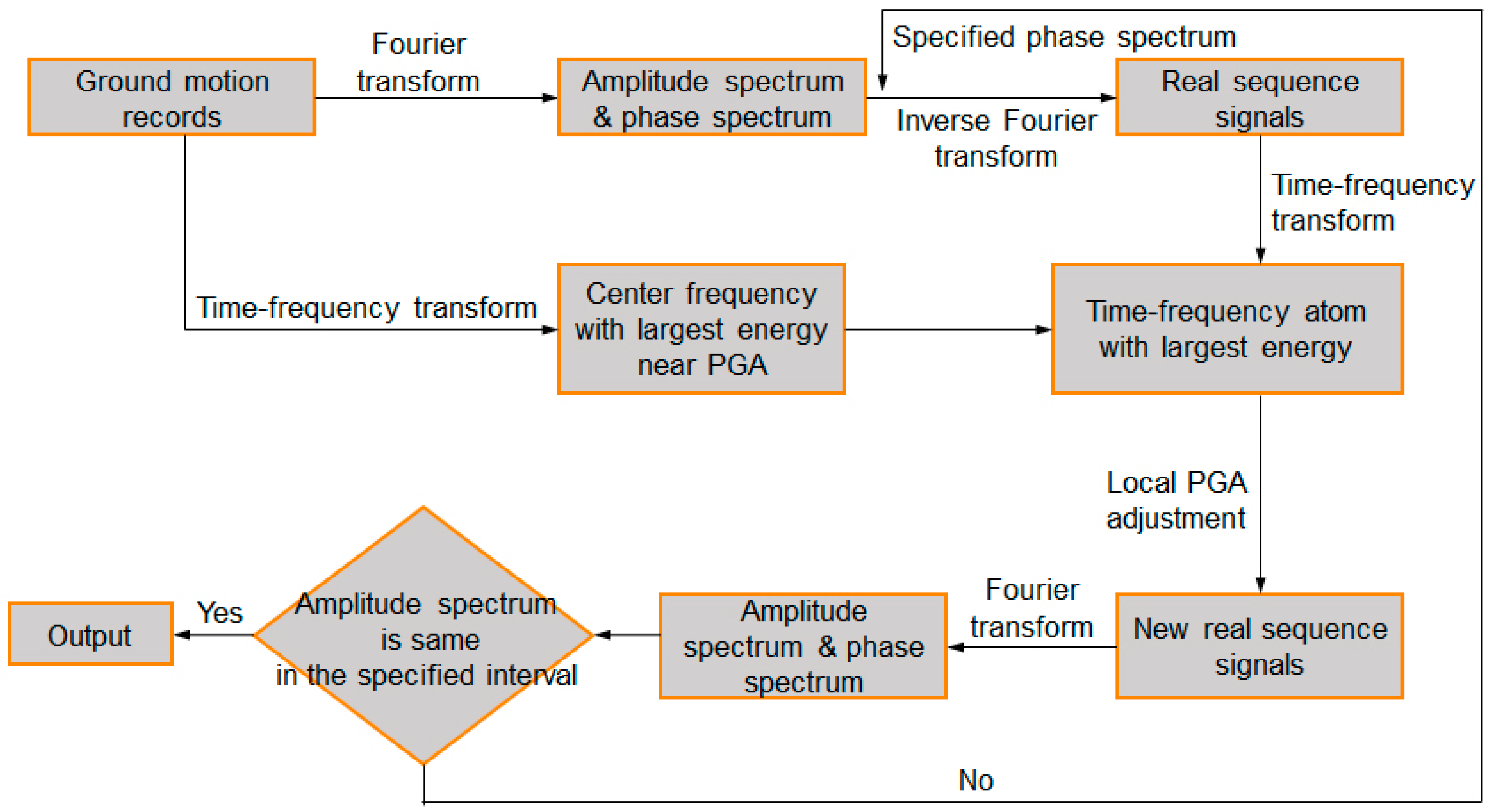
The above matching pursuit decomposition algorithm can be implemented by Matlab. Take an actual earthquake ground motion (Hachinohe) for example, the time-frequency energy distribution obtainment flow chart is shown in Figure 1. Due to the adaptability of the algorithm, the time-frequency energy distribution obtained by the matching pursuit decomposition algorithm has a relatively high time and frequency resolution.
3. Dynamic Ratcheting Phenomena
Dynamic ratcheting usually occurs in nonlinear systems. It means the structural plastic deformation may accumulate in a certain direction under certain excitations, which makes the structure produce large nonlinear displacement. The excessive displacement under seismic excitation may even cause progressive collapse, which should be avoided in practical projects. In order to facilitate the reader to understand the dynamic ratcheting phenomenon, this section briefly introduces the origination of dynamic ratcheting as follows.
The equation of motion for an elasto-perfectly-plastic single degree of freedom structure is given by Equation (12).
where is the nonlinear restoring force, satisfying:
where is the structure yield force.
Structure ductility is:
where is the structural yield displacement.
Assuming , then
Substituting into Equation (12) obtains the equation of ductility, shown in Equation (16).
where is the damping ratio; is the angular frequency before yield.
Take simple sinusoidal excitation as an example to explore the origination of the dynamic ratcheting phenomenon of an elasto-perfectly-plastic structure. Input is given by Equation (17).
where is the fundamental frequency of the sinusoidal excitation; is the frequency ratio of two input excitation.
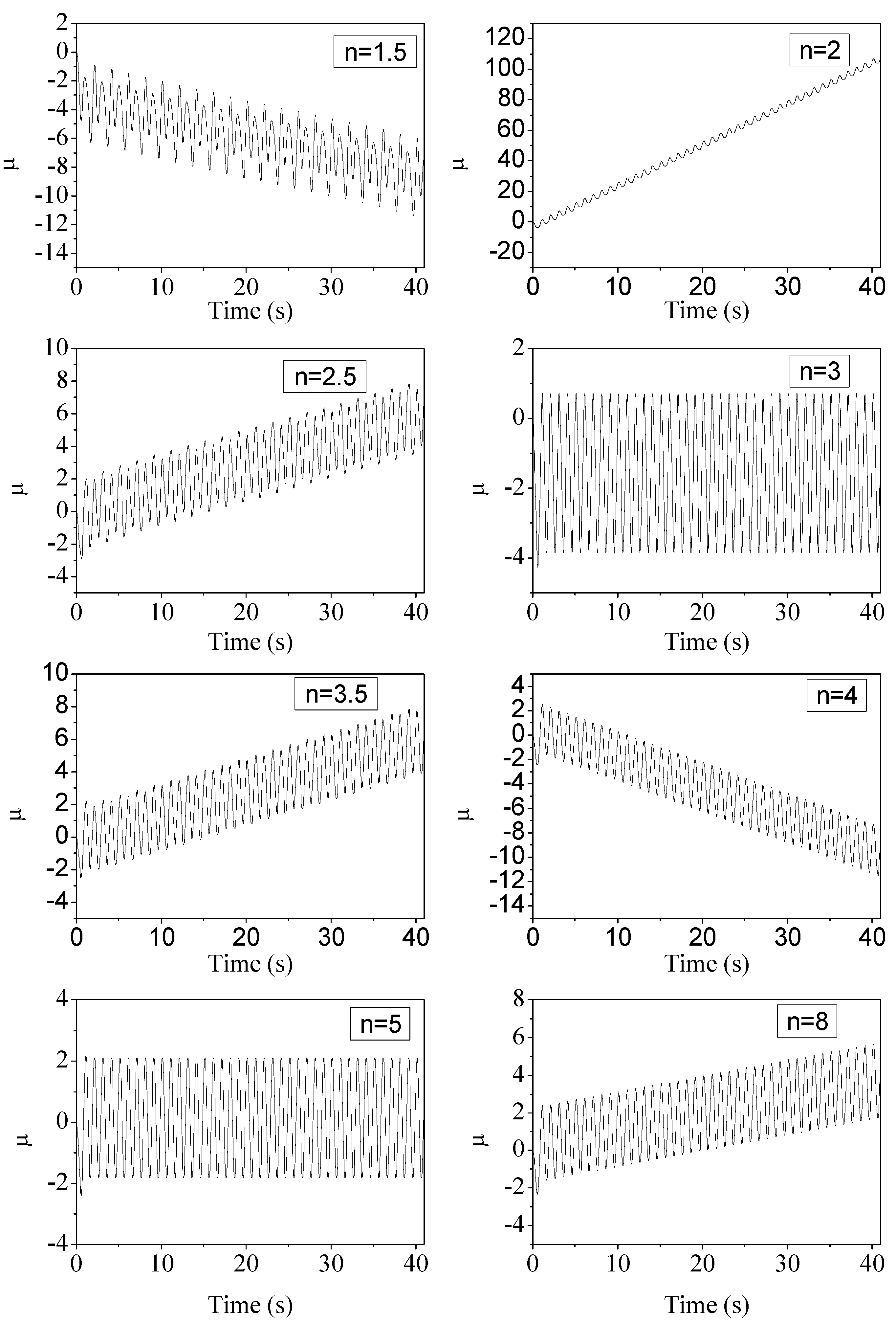
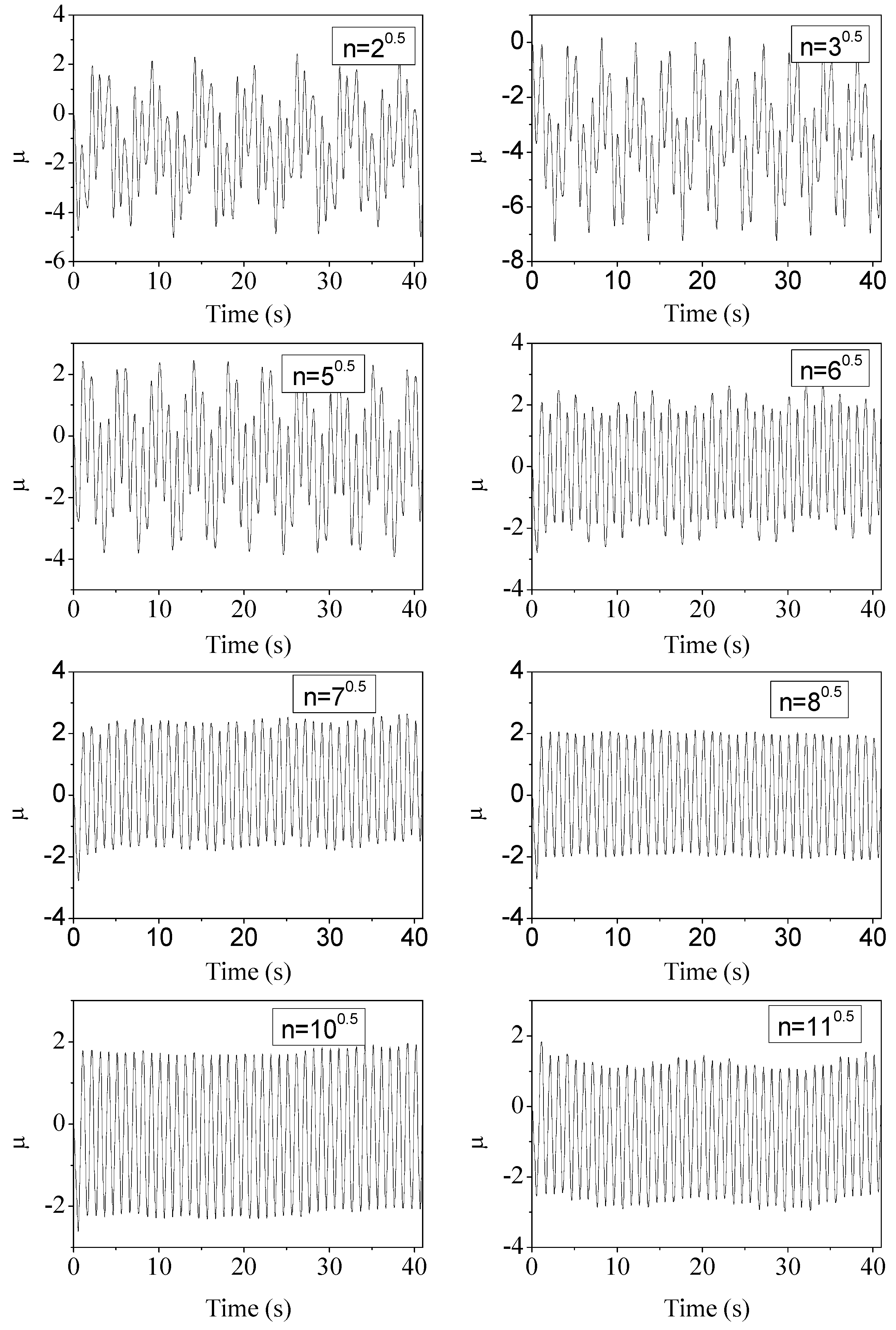
Supposing an elasto-perfectly-plastic structure model, whose mass is 1 kg, yield displacement is 0.01 m, structural frequency before yielding is 1 Hz, and the damping ratio is 0.05. Excite the elasto-perfectly-plastic structure by two sine waves. Since the fundamental frequency of the sine waves is 1 Hz, when the frequency ratio is rational, e.g., and respectively, the ductility time-history is shown in Figure 2; when the frequency ratio is irrational, e.g., , , , , , , and respectively, the ductility time-history is shown in Figure 3. It can be seen from Figure 2 that when the frequency ratio is even, the dynamic ratcheting phenomenon is obvious, and the dynamic ratcheting effect is more significant with a smaller frequency ratio, and when the frequency ratio is 2 the structural ductility demand is far more than other cases. On the other hand, it is known from Figure 3 that when the frequency ratio is irrational, dynamic ratcheting does not occur.
In conclusion, the elasto-perfectly-plastic structure shows a very significant dynamic ratcheting phenomenon under sinusoidal excitation with a frequency ratio of 2; but this requires the multiple frequencies occurring within the same time period, if not at the same time, even if the frequency ratio is 2, there will be no dynamic ratcheting.
4. Influence of Time-Frequency Energy Distribution of Ground motion on Structural Response
This section aims to analyze the influence of the time-frequency characteristics of ground motion on the structural response. It is well known that as structural members yielded, the dominant frequency of the nonlinear structure decreased [42,43], which may cause a resonance if the dominant frequency being equal to the time-varying frequency of the earthquake ground motion. Moreover, if the earthquake ground motion has multiple frequency components at the same time period, the dynamic ratcheting phenomenon will occur, resulting in a large nonlinear displacement of the structure [44,45,46]. For simplicity, only the elasto-perfectly-plastic structure is considered in this paper. The seismic nonlinear response of a practical project is much more complex.
4.1. Influence of Time-Frequency Energy Distribution of Simple Input on Structural Response
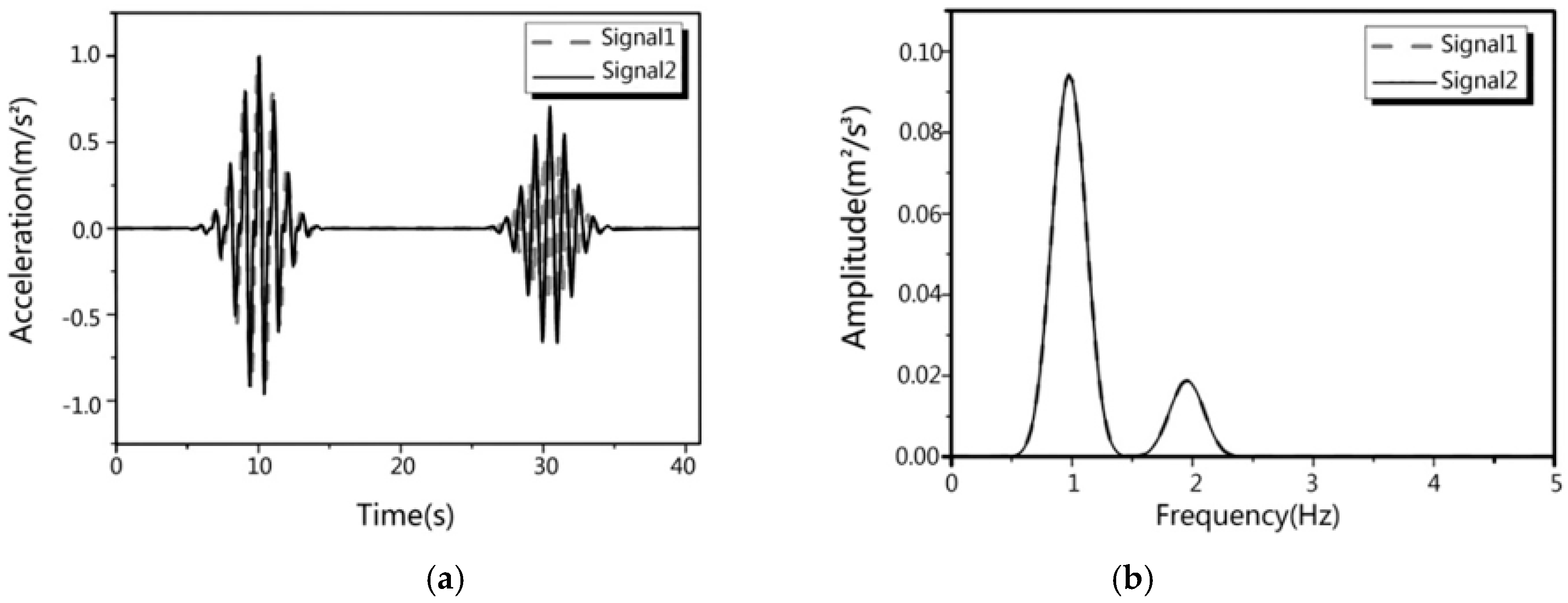
Construct two artificial signals with the same peak acceleration, duration, and power spectrum, but different time-frequency energy distributions. The power spectrum is considered here instead of the spectrum to prevent spectral leakage. The two signals have a sampling frequency of 100 Hz and the signal duration of 40.95 s. The peak ground acceleration (PGA) of the first signal is 1 m/s2 at the time instant 9.99 s; the PGA of the second signal is also 1 ms−2, while at the time instant 10.09 s. When using a 512-point Hanning window, a 256-point overlap, and the 4096-point Fast Fourier Transform, the smooth power spectrum density of the two signals is the same at 0–5 Hz. Their time history and smoothed power spectrum are shown in Figure 4.
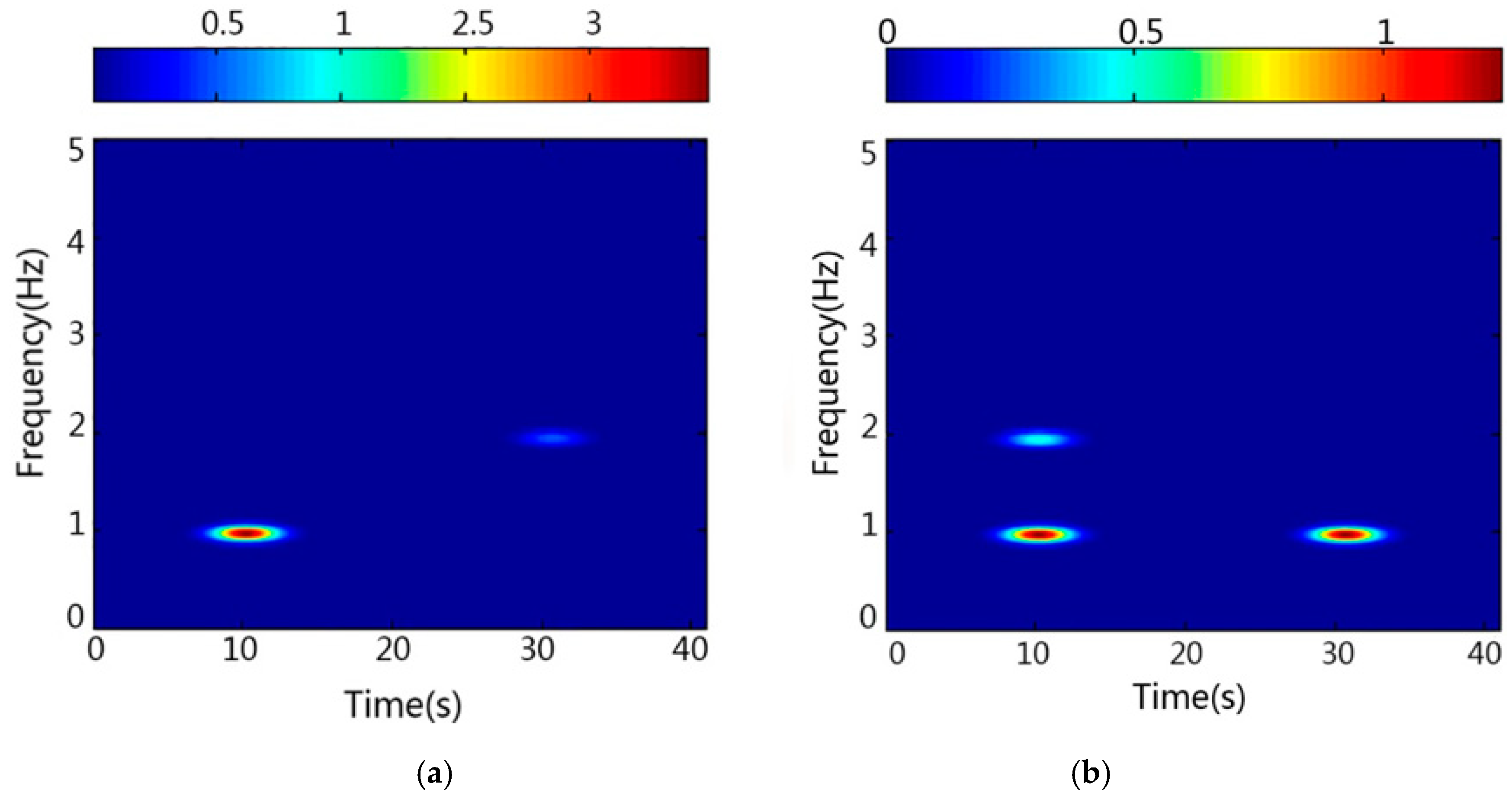
The time-frequency energy distribution of the above signals obtained by the matching pursuit decomposition is shown in Figure 5. It can be seen that although the smooth power spectra of the two signals are exactly the same, the respective frequency evolution processes are fairly different, so are the corresponding time-frequency energy distribution maps. The energy of the first signal in the 1 Hz band is concentrated within 5–15 s, and the energy in the 2 Hz band is concentrated in 25–35 s; while the energy of the second signal in the 1 Hz band is concentrated in both 5–15 s and 25–35 s, the energy in the 2 Hz band is concentrated within 5–15 s.
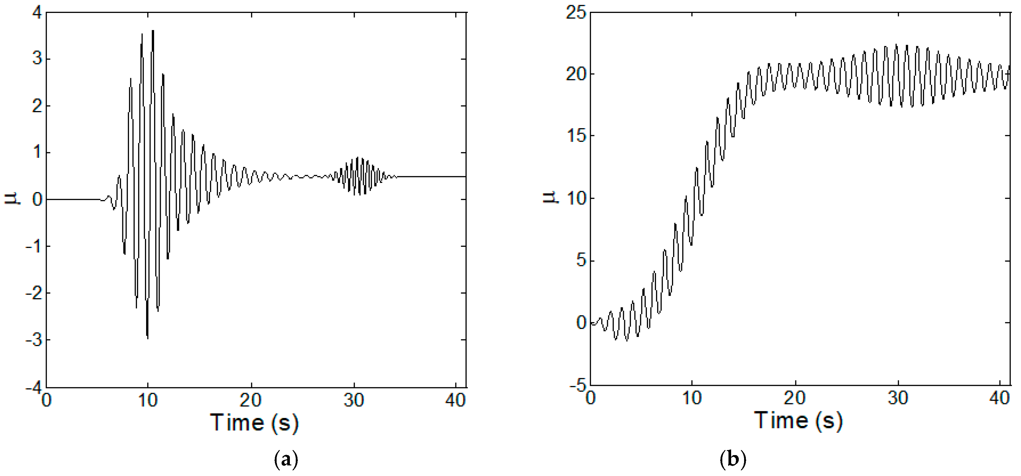
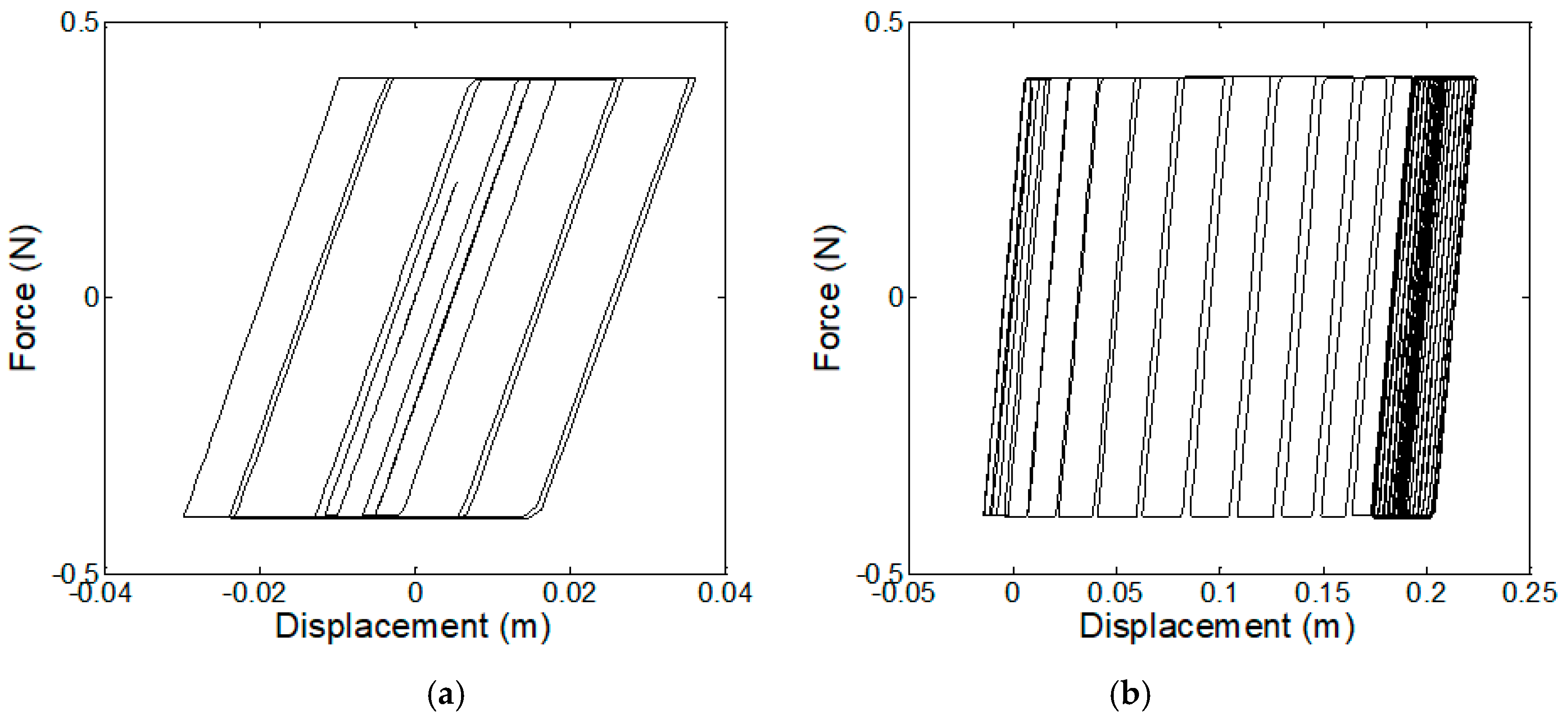
Analyze the structural response of the above elasto-perfectly-plastic structure under the two simple artificial signals. The ductility time history is shown in Figure 6, and the force-displacement relationship is shown in Figure 7, respectively.
It can be seen from Figure 6 that the ductility of the elasto-perfectly-plastic structure under the second signal is much larger than that under the first one. The former has a peak ductility of more than 20 and a residual ductility of about 20; while the latter has a peak ductility of no more than 5 and a residual ductility of about 0.5. According to the time-frequency energy distribution (Figure 5), the second signal has both the energy of 1 Hz band and 2 Hz band concentrated in 5–15 s, and the frequency ratio is 2, resulting in dynamic ratcheting phenomenon; since there is only a 1 Hz band energy in 25–35 s, dynamic ratcheting phenomenon does not occur in the period of 25-35 s. In comparison, the first signal has only the 1 Hz band energy concentrated in 5–15 s, and only 2 Hz band energy in 25–35 s respectively. Without multiple frequencies occurring within the same time period, the structure does not show dynamic ratcheting under the first signal. This indicates that the occurrence of structural dynamic ratcheting is closely related to the time-frequency energy distribution input.
Meanwhile, the force-displacement curve in Figure 7a is more symmetrical, and the curve is more evenly distributed around zero displacement point; while the force-displacement curve in Figure 7b is concentrated on the right side of zero displacement point with a residual displacement of 0.2 m. This shows that the time-frequency energy distribution of the input signal has a great influence on the ductile response of the elasto-perfectly-plastic structure, and if there are frequency components with even frequency ratio at the same time, the structure may have a complex response such as a dynamic ratcheting effect.
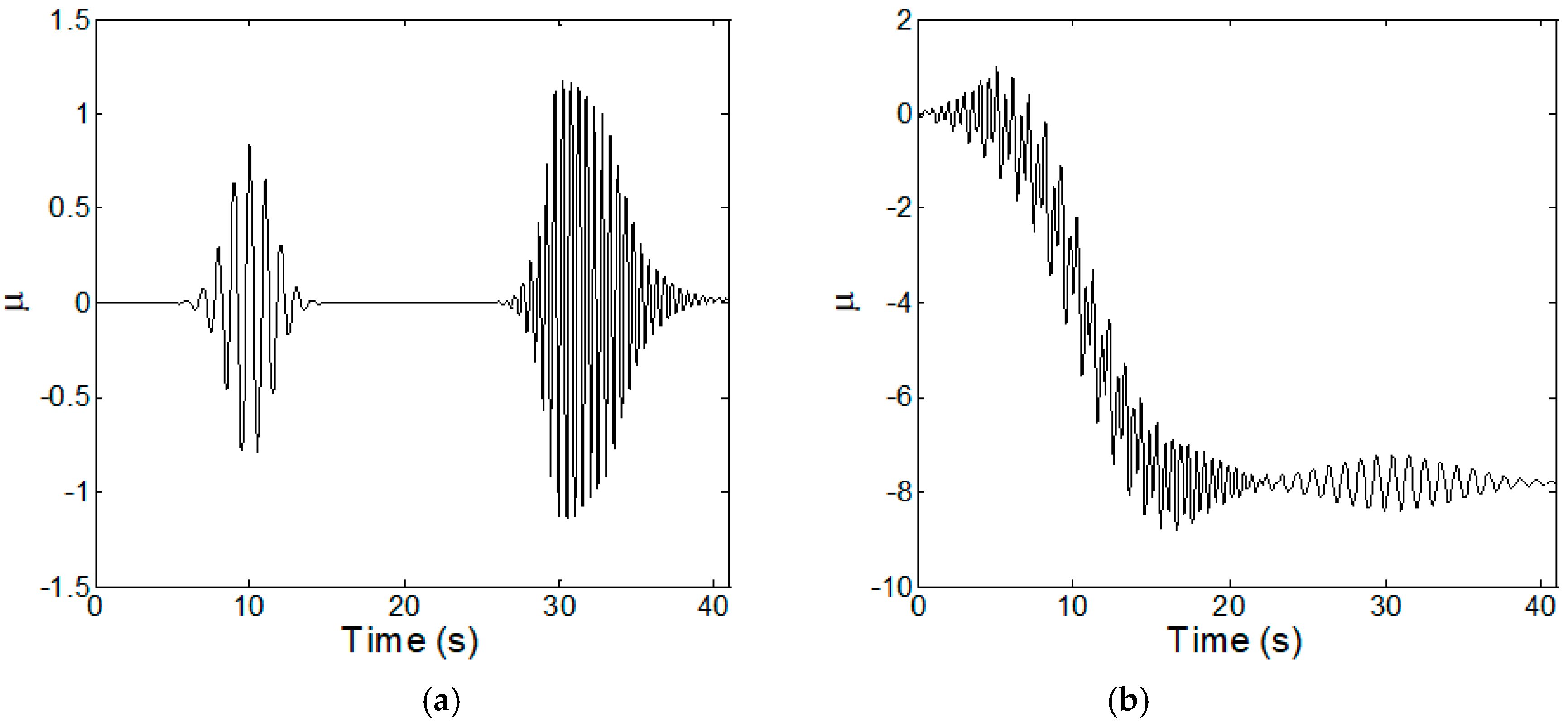
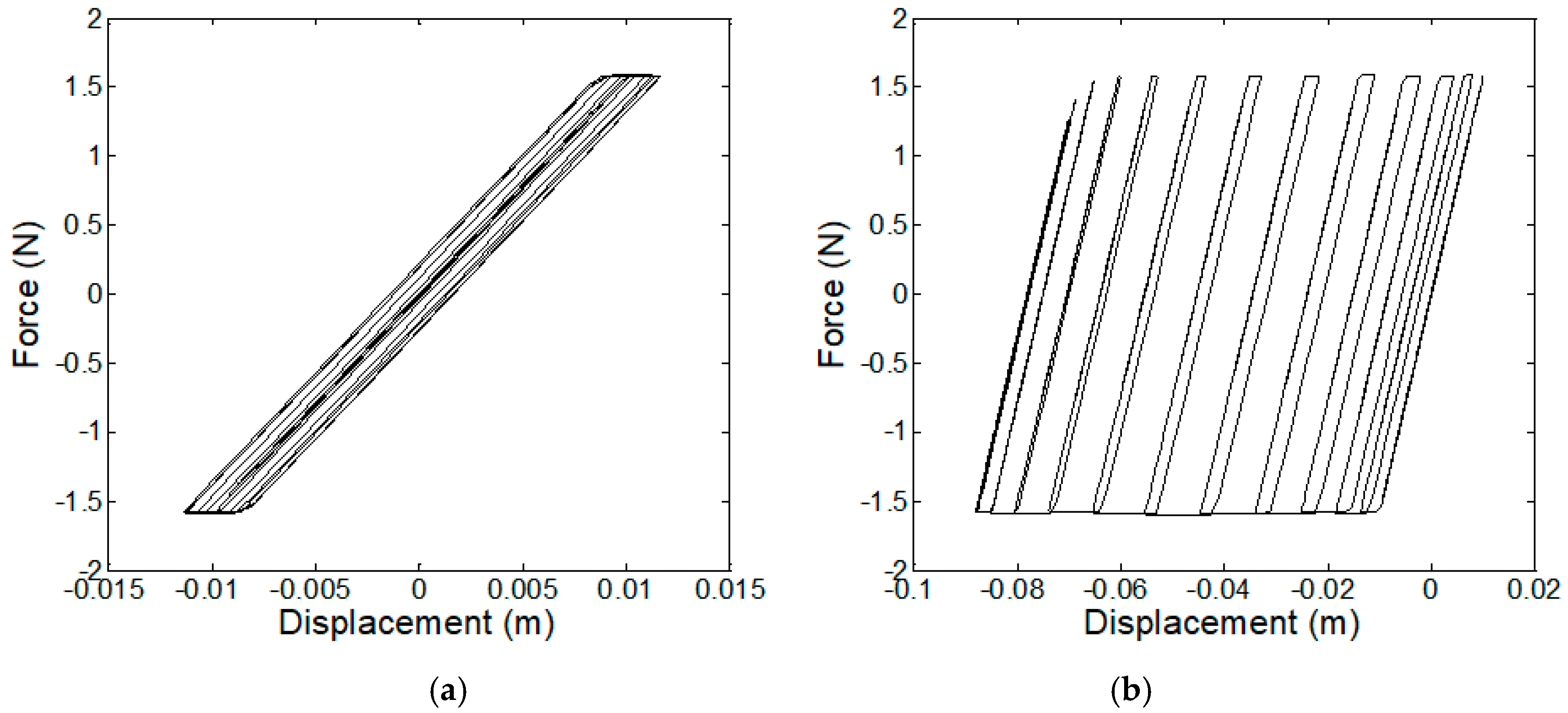
When the elasto-perfectly-plastic structure frequency is 2 Hz before yielding and the yield displacement is 0.01 m, the structure ductility time history under the two artificial signals is shown in Figure 8, and the force-displacement relationship is shown in Figure 9. Results show that the structure also experienced dynamic ratcheting under the second signal, due to the fact that the second signal has both the energy of 1 Hz band and 2 Hz band in 5-15 s, and the frequency ratio is even, thereby the dynamic ratcheting phenomenon occurs.
4.2. Influence of Time-Frequency Energy Distribution of Ground Motion on Structural Response
Since it is difficult to find an actual earthquake ground motion with the same ground motion parameters as the above constructed two signals, this section constructs a series of artificial ground motions based on the actual earthquake ground motion records. Similarly, we construct the artificial ground motions with the same peak acceleration, spectral characteristics, and duration to fully analyze the seismic effect of the energy distribution of the ground motion.
The artificial earthquake ground motion generation flow chart is shown in Figure 10. The basic idea is that the Fourier amplitude spectra of the generated ground motions are from those of typical earthquake ground motions (for simplicity these ground motions are noted as GM-A) and the phase spectra are from those of ground motions with PGA larger than a certain value like 0.2 g (for simplicity these ground motions noted as GM-B). The generation procedures in details are as follows:
(1) Take Fourier transform of GM-A and get the amplitude and phase spectrum, meanwhile take time-frequency transform to get the center frequency with the largest time frequency atom near the time instant when PGA occurs;
(2) Substitute the phase spectrum of GM-A by that of GM-B and make an inverse Fourier transform to get the real sequence signals and take the time-frequency transform of the generated real sequence signals and get the time-frequency atom with the largest energy.
(3) Replace the time-frequency atom with largest energy by that of GM-A, and adjust the local PGA thus that the PGA of the new generated real time sequence is equal to that of GM-A;
(4) Take the Fourier transform of the new generated sequence signal to get the amplitude and phase spectrum and to check if the amplitude spectrum is same as that of GM-A in the specified interval. If it is true, the new generated sequence signal is a passable artificial earthquake ground motion. Otherwise modify the phase spectrum and go back to step (2).
In this study, the typical earthquake ground motion records referred to Chichi, El Centro, Northridge, Parkfield, and the Kobe earthquake ground motion records and their peak accelerations and peak frequencies are shown in Table 1. The phase spectra referred to the records in the horizontal direction with peak accelerations larger than 0.2 g in the Chichi, Imperial Valley, Northridge, Parkfield, and Kobe earthquakes, as shown in Table 2, for a total of 169 records.
Model an elasto-perfectly-plastic structure with a before-yielding frequency of 1 Hz, a yield displacement of 0.01 m, a damping ratio of 0.05, and a mass of 1 kg. Excite the structure by the generated artificial ground motions. If the ductility time history of the structure is provided with these characteristics: (1) The maximum ductility coefficient is greater than 3; (2) the plastic deformation of the structure continuously accumulates in a certain direction and the duration is greater than the three before-yielded period of the structure; the structure dynamic ratcheting phenomenon occurs. As a result, there are only seven artificial seismic waves generated according to above procedures, leading to the structural dynamic ratcheting phenomenon. The referred earthquake ground motion records are shown in Table 3.
Take CHY006-E and KAK090 for example to analyze the effect of the time-frequency energy distribution on the structural nonlinear response.
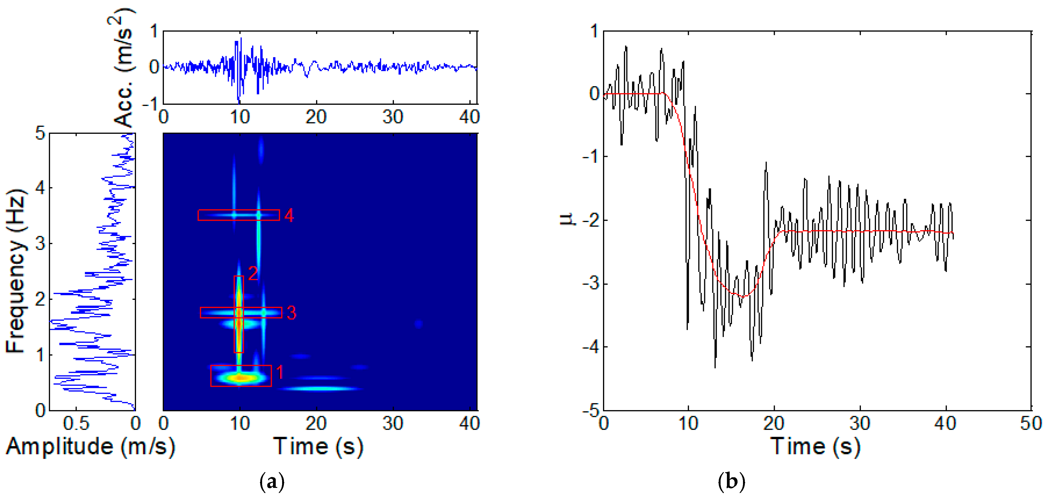
The time-frequency energy distribution of the CHY006-E ground motion is shown in Figure 11a. The ductility of the elasto-perfectly-plastic structure is shown in Figure 11b. As shown in Figure 11a, the center frequencies of the time-frequency atom #1, #2, #3, and #4, are 0.586 Hz, 1.563 Hz, 1.758 Hz, and 3.516 Hz, respectively. Not only that the atomic center frequency of the atom #2 is twice the center frequency of #1; similarly that of the atom #4 is twice of #3. It can be seen from Figure 11b that the dynamic ratcheting phenomenon occurs within 9–18 s, which is consistent with the time-frequency energy distribution in Figure 11a, because it exists time-frequency atoms whose center frequency ratio is twice during the period. Besides, no dynamic ratcheting occurred during other periods.
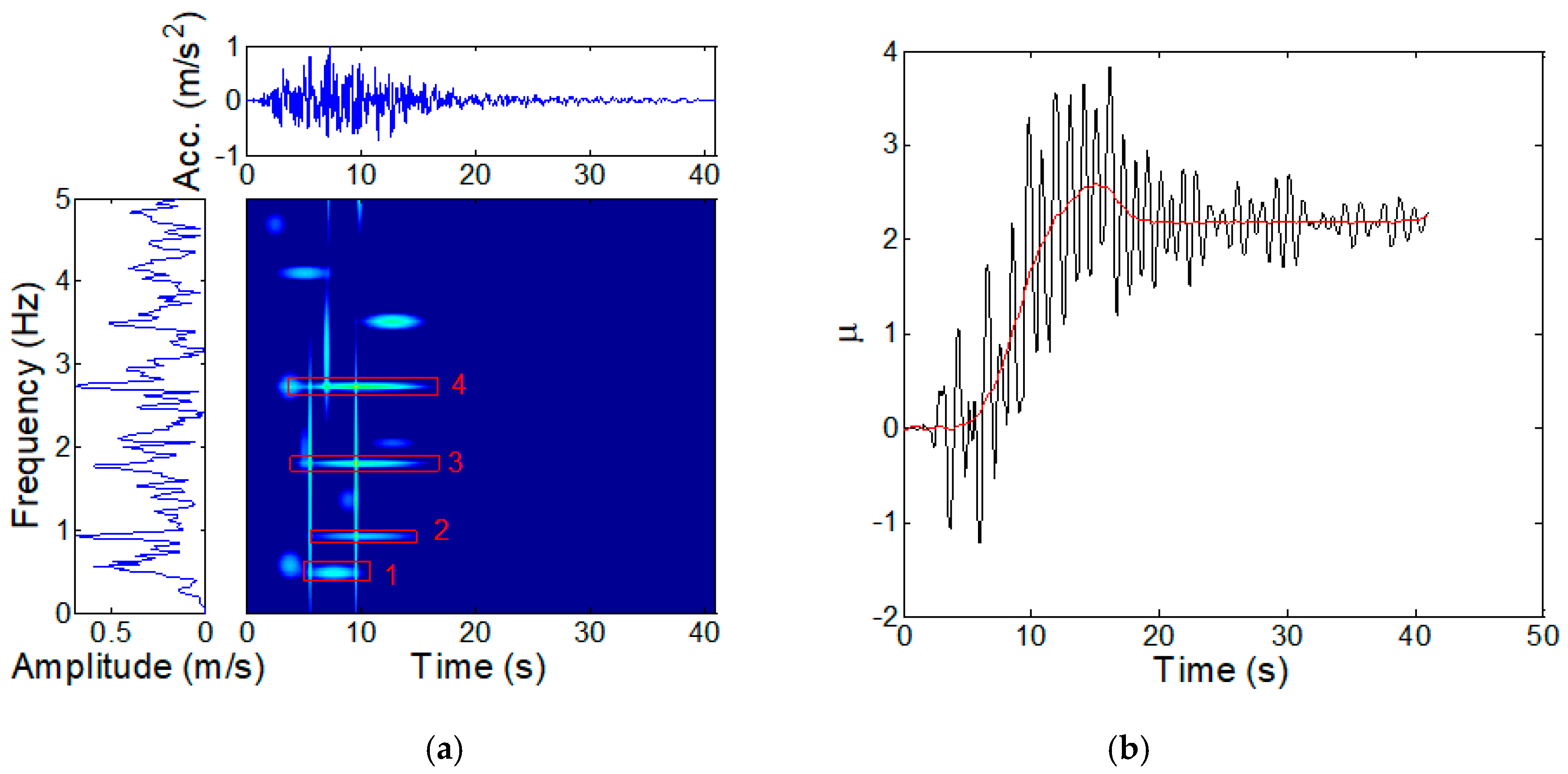
The time-frequency energy distribution of the KAK090 ground motion is shown in Figure 12a. The ductility of the elasto-perfectly-plastic structure is shown in Figure 12b. As shown in Figure 12a, the center frequencies of the time-frequency atom #1, #2, #3, #4 are 0.488 Hz, 0.976 Hz, 1.824 Hz, and 2.734 Hz respectively. Moreover the atomic center frequency of the atom #2 is twice the center frequency of #1; and that of the atom #4 is 1.5 times of #3. It can be seen from Figure 12b that the dynamic ratcheting phenomenon occurs within 6–14 s, which is consistent with the time-frequency energy distribution in Figure 12a, because there is time-frequency atoms whose center frequency ratio is twice and 1.5 times during the period. Besides, no dynamic ratcheting occurred during other periods as well.
5. Conclusions
This paper proposes an earthquake ground motion generation method based on the matching pursuit decomposition algorithm and time-frequency energy distribution; constructs a series of simple signals and artificial earthquake ground motions with the same peak ground acceleration, Fourier amplitude spectrum, and duration; explains the dynamic ratcheting phenomenon of the elasto-perfectly-plastic structure. The main conclusions are as follows:
(1) The proposed decomposition for the earthquake ground motion has both high time resolution and high frequency resolution. The obtained time-frequency energy distribution can effectively reflect the energy distribution of the frequency components at any time and also reflect the frequency components near the peak acceleration.
(2) If there are frequency components with an even frequency ratio in a certain time duration, the response of the elasto-perfectly-plastic structure experiences a dynamic ratchet phenomenon. If these frequency components appear at different time periods, the elasto-perfectly-plastic structure does not undergo dynamic ratcheting.
(3) The time-frequency energy distribution could be further considered as a characteristic variable for ground motion besides peak ground acceleration, frequency spectrum, and duration, which has a vital effect on the structural response, especially in the nonlinear range.
Author Contributions
Funding acquisition, Z.L.; investigation, D.T.; project administration, D.T. and Z.L.; software, D.T. and J.L.; writing – original draft, J.L.; writing – review and editing, Z.L.
Funding
This research was funded by Scientific Research Fund of Institute of Engineering Mechanics, China Earthquake Administration, grant number 2018D01, 2014B08, 2016A03. This research was also funded by China Scholarship Council, grant number 201704190039. The APC was funded by Scientific Research Fund of Institute of Engineering Mechanics, China Earthquake Administration, grant number 2018D01, 2014B08, 2016A03.
Acknowledgments
Financial support from the Scientific Research Fund of Institute of Engineering Mechanics, China Earthquake Administration (Grant No. 2018D01, 2014B08, 2016A03) is highly appreciated. The work is also supported by the China Scholarship Council (Grant No. 201704190039).
Conflicts of Interest
The authors declare no conflict of interest.
References
- Lu, Z.; Chen, X.Y.; Lu, X.L. Shaking table test and numerical simulation of an RC frame-core tube structure for earthquake-induced collapse. Earthq. Eng. Struct. Dyn. 2016, 45, 1537–1556. [Google Scholar] [CrossRef]
- Spencer, B.F.; Yao, J.T.P. Structural control: Past, present, and future. J. Eng. Mech. (ASCE) 1997, 123, 897–971. [Google Scholar]
- Spencer, B.F., Jr.; Nagarajaiah, S. State of the Art of Structural Control. J. Struct. Eng. 2003, 129, 845–856. [Google Scholar] [CrossRef]
- Housner, G.W.; Bergman, L.A.; Caughey, T.K.; Chassiakos, A.G.; Claus, R.O.; Masri, S.F.; Skelton, R.E.; Soong, T.T.; Li, S.; Tang, J. On vibration suppression and energy dissipation using tuned mass particle damper. J. Vib. Acoust. 2017, 139, 011008. [Google Scholar]
- Lu, Z.; Chen, X.Y.; Li, X.W.; Li, P.Z. Optimization and application of multiple tuned mass dampers in the vibration control of pedestrian bridges. Struct. Eng. Mech. 2017, 62, 55–64. [Google Scholar] [CrossRef]
- Lu, Z.; Chen, X.Y.; Zhou, Y. An equivalent method for optimization of particle tuned mass damper based on experimental parametric study. J. Sound Vib. 2018, 419, 571–584. [Google Scholar] [CrossRef]
- Lu, Z.; Huang, B.; Zhou, Y. Theoretical study and experimental validation on the energy dissipation mechanism of particle dampers. Struct. Control Health Monit. 2018, 25, e2125. [Google Scholar] [CrossRef]
- Hu, Y.X. Earthquake Engineering; Seismological Press: Beijing, China, 2006; pp. 380–382. [Google Scholar]
- Bozorgnia, Y.; Bertero, V.V. Earthquake Engineering: From Engineering Seismology to Performance-Based Engineering; CRC Press: Boca Raton, FL, USA, 2004. [Google Scholar]
- Cacciola, P.; Deodatis, G. A method for generating fully non-stationary and spectrum-compatible ground motion vector processes. Soil Dyn. Earthq. Eng. 2011, 31, 351–360. [Google Scholar] [CrossRef] [Green Version]
- Sgobba, S.; Stafford, P.; Marano, G.; Guaragnella, C. An evolutionary stochastic ground-motion model defined by a seismological scenario and socal site conditions. Soil Dyn. Earthq. Eng. 2011, 31, 1465–1479. [Google Scholar] [CrossRef]
- Zentner, I.; Poirion, F. Enrichment of seismic ground motion databases using Karhunen–Loève expansion. Soil Dyn. Earthq. Eng. 2012, 41, 1945–1957. [Google Scholar] [CrossRef]
- Zhang, Y.; Zhao, F.; Yang, C. Generation of nonstationary artificial ground motion based on the Hilbert transform. Bull. Seismol. Soc. Am. 2012, 102, 2405–2419. [Google Scholar] [CrossRef]
- Rezaeian, S.; Der Kiureghian, A. Simulation of orthogonal horizontal ground motion components for specified earthquake and site characteristics. Soil Dyn. Earthq. Eng. 2012, 41, 335–353. [Google Scholar] [CrossRef]
- Iyama, J.; Kuwamura, H. Application of wavelets to analysis and simulation of earthquake motions. Soil Dyn. Earthq. Eng. 1999, 28, 255–272. [Google Scholar] [CrossRef]
- Beck, J.L.; Papadimitriou, C. Moving resonance in nonlinear response to fully nonstationary stochastic ground motion. Probab. Eng. Mech. 1993, 8, 157–167. [Google Scholar] [CrossRef]
- Stockwell, R.G.; Mansinha, L.; Lowe, R. Localization of the complex spectrum: The S transform. IEEE Trans. Signal Process. 1996, 44, 998–1001. [Google Scholar] [CrossRef]
- Wu, Z.J.; Zhang, J.J.; Wang, Z.J.; Wu, X.X.; Wang, M.Y. Time-frequency analysis on amplification of seismic ground motion. Rock Soil Mech. 2017, 138, 685–695. [Google Scholar]
- Zhang, Y.S.; Zhao, F.X. Validation of non-stationary ground motion simulation method based on Hilbert transform. Acta Seismol. Sin. 2014, 36, 686–697. [Google Scholar]
- Wang, D.; Fan, Z.L.; Hao, S.W.; Zhao, D.H. An evolutionary power spectrum model of fully nonstationary seismic ground motion. Soil Dyn. Earthq. Eng. 2018, 105, 1–10. [Google Scholar] [CrossRef]
- Naga, P.; Eatherton, M.R. Analyzing the effect of moving resonance on seismic response of structures using wavelet transforms. Soil Dyn. Earthq. Eng. 2013, 43, 759–768. [Google Scholar] [CrossRef] [Green Version]
- Yazdani, A.; Takada, T. Wavelet-based generation of energy- and spectrum-compatible earthquake time histories. Comput.-Aided Civ. Infrastruct. Eng. 2009, 24, 623–630. [Google Scholar] [CrossRef]
- Sun, D.B.; Ren, Q.W. Seismic damage analysis of concrete gravity dam based on wavelet transform. Shock Vib. 2016, 2016, 6841836. [Google Scholar] [CrossRef]
- Altunisik, A.C.; Genc, A.F.; Gunaydin, M.; Okur, F.Y.; Karahasan, O.S. Dynamic response of a historical armory building using the finite element model validated by the ambient vibration test. J. Vib. Control 2018, 24, 5472–5484. [Google Scholar] [CrossRef]
- Bai, Y.T.; Guan, S.Y.; Lin, X.C.; Mou, B. Seismic collapse analysis of high-rise reinforced concrete frames under long-period ground motions. Struct. Des. Tall Spec. Build. 2019, 28, e1566. [Google Scholar] [CrossRef]
- Han, Q.; Wen, J.N.; Du, X.L.; Zhong, Z.L.; Hao, H. Nonlinear seismic response of a base isolated single pylon cable-stayed bridge. Eng. Struct. 2018, 175, 806–821. [Google Scholar] [CrossRef]
- Li, X.Q.; Li, Z.X.; Crewe, A.J. Nonlinear seismic analysis of a high-pier, long-span, continuous RC frame bridge under spatially variable ground motions. Soil Dyn. Earthq. Eng. 2018, 114, 298–312. [Google Scholar] [CrossRef]
- Cao, H.; Friswell, M.I. The effect of energy concentration of earthquake ground motions on the nonlinear response of RC structures. Soil Dyn. Earthq. Eng. 2009, 29, 292–299. [Google Scholar] [CrossRef]
- Yu, R.F.; Fan, K.; Peng, L.Y.; Yuan, M.Q. Effect of non-stationary characteristics of ground motion on structural response. China Civ. Eng. J. 2010, 43, 13–20. [Google Scholar]
- Zhang, S.R.; Du, Y.F.; Hui, Y.X. Seismic response analysis of isolation structures based on wavelet transformation. China Earthq. Eng. J. 2017, 39, 836–842. [Google Scholar]
- Yaghmaei-Sabegh, S. Time-frequency analysis of the 2012 double earthquakes records in north-west of Iran. Bull. Earthq. Eng. 2014, 12, 585–606. [Google Scholar] [CrossRef]
- Mallat, S.G.; Zhang, Z.F. Matching pursuits with time-frequency dictionaries. IEEE Trans. Signal Proc. 1993, 41, 3397–3415. [Google Scholar] [CrossRef] [Green Version]
- Neff, R.; Zakhor, A. Very low bit-rate video coding based on matching pursuits. IEEE Trans. Circuits Syst. Video Technol. 1997, 7, 158–171. [Google Scholar] [CrossRef] [Green Version]
- Gribonval, R. Fast matching pursuit with a multiscale dictionary of Gaussian chirps. IEEE Trans. Signal Proc. 2001, 49, 994–1001. [Google Scholar] [CrossRef] [Green Version]
- Gribonval, R.; Bacry, E. Harmonic decomposition of audio signals with matching pursuit. IEEE Trans. Signal Proc. 2003, 51, 101–111. [Google Scholar] [CrossRef] [Green Version]
- Tropp, J.A.; Gilbert, A.C. Signal recovery from random measurements via orthogonal matching pursuit. IEEE Trans. Signal Proc. 2007, 53, 4655–4666. [Google Scholar] [CrossRef]
- Needell, D.; Vershynin, R. Signal recovery from incomplete and inaccurate measurements via regularized orthogonal matching pursuit. IEEE J. Sel. Top. Signal Proc. 2010, 4, 310–316. [Google Scholar] [CrossRef]
- Yang, B.; Li, S.T. Pixel-level image fusion with simultaneous orthogonal matching pursuit. Inf. Fusion 2012, 13, 10–19. [Google Scholar] [CrossRef]
- Liu, X.Y.; Zhao, Z.G. Research on compressed sensing reconstruction algorithm in complementary space. In Proceedings of the IEEE 17th International Conference on Communication Technology (ICCT), Chengdu, China, 27–30 October 2017. [Google Scholar]
- Charles, I.P.; John, P.C. Comparison of frequency attributes from CWT and MPD spectral decompositions of a complex turbidite channel model. In Proceedings of the Expanded Abstracts of 78th SEG Annual International Meeting, Las Vegas, NV, USA, 9–14 November 2008; pp. 394–397. [Google Scholar]
- Tao, D.W.; Li, H. Time-frequency energy distribution of wenchuan earthquake motions based on matching pursuit decomposition. In Proceedings of the 7th International Conference on Urban Earthquake Engineering (7CUEE) & 5th International Conference on Earthquake Engineering (5ICEE), Tokyo, Japan, 3–5 March 2010. [Google Scholar]
- Montejo, L.A.; Kowalsky, M.J. Estimation of frequency-dependent strong motion duration via wavelets and its influence on nonlinear seismic response. Comput.-Aided Civ. Infrastruct. Eng. 2008, 23, 253–264. [Google Scholar] [CrossRef]
- Chandramohan, R.; Baker, J.W.; Deierlein, G.G. Quantifying the influence of ground motion duration on structural collapse capacity using spectrally equivalent records. Earthq. Spectra 2016, 43, 927–950. [Google Scholar] [CrossRef]
- Ahn, I.S.; Chen, S.S.; Dargush, G.F. Dynamic ratcheting in elastoplastic SDOF systems. J. Eng. Mech. 2006, 132, 411–421. [Google Scholar] [CrossRef]
- Challamel, N.; Lanos, C.; Hammouda, A.; Redjel, B. Stability analysis of dynamic ratcheting in elastoplastic systems. Phys. Rev. E 2007, 75, 026204. [Google Scholar] [CrossRef]
- Ahn, I.S.; Chen, S.S.; Dargush, G.F. An iterated maps approach for dynamic ratchetting in SDOF hysteretic damping systems. J. Sound Vib. 2009, 323, 896–909. [Google Scholar] [CrossRef]
Figure 1.
Flowchart of obtaining the time-frequency energy distribution.

Figure 2.
Ductility of Elasto-Perfectly-Plastic model under sine waves with rational frequency ratio (structural frequency is 1 Hz before yielding).
Figure 2.
Ductility of Elasto-Perfectly-Plastic model under sine waves with rational frequency ratio (structural frequency is 1 Hz before yielding).

Figure 3.
Ductility of Elasto-Perfectly-Plastic model under sine waves with irrational frequency ratio (structural frequency is 1 Hz before yielding).
Figure 3.
Ductility of Elasto-Perfectly-Plastic model under sine waves with irrational frequency ratio (structural frequency is 1 Hz before yielding).

Figure 4.
Two artificial signals with the same peak ground acceleration (PGA) and smoothed power spectrum density. (a) Time history. (b) Smoothed power spectrum density.
Figure 4.
Two artificial signals with the same peak ground acceleration (PGA) and smoothed power spectrum density. (a) Time history. (b) Smoothed power spectrum density.

Figure 5.
Time-frequency energy distribution of the two artificial signals. (a) First artificial signal. (b) Second artificial signal.
Figure 5.
Time-frequency energy distribution of the two artificial signals. (a) First artificial signal. (b) Second artificial signal.

Figure 6.
Ductility of the Elasto-Perfectly-Plastic model under the two artificial signals (structural frequency is 1 Hz before yielding). (a) First artificial signal. (b) Second artificial signal.
Figure 6.
Ductility of the Elasto-Perfectly-Plastic model under the two artificial signals (structural frequency is 1 Hz before yielding). (a) First artificial signal. (b) Second artificial signal.

Figure 7.
Force-displacement curve of the Elasto-Perfectly-Plastic model under the two artificial signals (structural frequency is 1 Hz before yielding). (a) First artificial signal. (b) Second artificial signal.
Figure 7.
Force-displacement curve of the Elasto-Perfectly-Plastic model under the two artificial signals (structural frequency is 1 Hz before yielding). (a) First artificial signal. (b) Second artificial signal.

Figure 8.
Ductility of Elasto-Perfectly-Plastic model under the two artificial signals (structural frequency is 2 Hz before yielding). (a) First artificial signal. (b) Second artificial signal.
Figure 8.
Ductility of Elasto-Perfectly-Plastic model under the two artificial signals (structural frequency is 2 Hz before yielding). (a) First artificial signal. (b) Second artificial signal.

Figure 9.
Force-displacement curve of Elasto-Perfectly-Plastic model under the two artificial signals (structural frequency is 2 Hz before yielding). (a) First artificial signal. (b) Second artificial signal.
Figure 9.
Force-displacement curve of Elasto-Perfectly-Plastic model under the two artificial signals (structural frequency is 2 Hz before yielding). (a) First artificial signal. (b) Second artificial signal.

Figure 10.
Flowchart of generating artificial ground motion.

Figure 11.
(a) Time-frequency energy distribution of CHY006-E ground motion. (b) Ductility of the Elasto-Perfectly-Plastic model under the CHY006-E ground motion.
Figure 11.
(a) Time-frequency energy distribution of CHY006-E ground motion. (b) Ductility of the Elasto-Perfectly-Plastic model under the CHY006-E ground motion.

Figure 12.
(a) Time-frequency energy distribution of KAK090 ground motion. (b) Ductility of Elasto-Perfectly-Plastic model under the KAK090 ground motion.
Figure 12.
(a) Time-frequency energy distribution of KAK090 ground motion. (b) Ductility of Elasto-Perfectly-Plastic model under the KAK090 ground motion.


Table 1.
Typical ground motion records.
| Site and Component, Ground Motion, Date | Peak Acceleration (g) | Peak Frequency (Hz) |
|---|---|---|
| TCU052-W, Chichi (20 September 1999) | 0.348 | 0.452 |
| I-ELC180, Imperial Valley (19 May 1940) | 0.313 | 1.465 |
| ORR090, Northridge (17 January 1994) | 0.568 | 1.221 |
| C02065, Parkfield (28 June 1966) | 0.476 | 1.428 |
| KJM000, Kobe (16 January 1995) | 0.821 | 1.453 |
Table 2.
Ground motion records generating the phase spectra.
| Ground Motion | Number of Ground Motion Records |
|---|---|
| Chichi (20 September 1999) | 71 |
| Imperial Valley (19 May 1940) | 2 |
| Kobe (16 January 1995) | 12 |
| Northridge (17 January 1994) | 77 |
| Parkfield (28 June 1966) | 7 |
Table 3.
Ground motion records generating dynamic ratcheting.
| Site and Component, Ground Motion, Date | Peak Acceleration (g) | Peak Frequency (Hz) |
|---|---|---|
| CHY006-E,Chichi (20 September 1999) | 0.364 | 0.595 |
| CHY028-N,Chichi (20 September 1999) | 0.821 | 1.190 |
| CHY029-N,Chichi (20 September 1999) | 0.238 | 0.354 |
| CHY029-W,Chichi (20 September 1999) | 0.277 | 0.403 |
| CHY101-W,Chichi (20 September 1999) | 0.353 | 0.336 |
| I-ELC180,Imperial Valley (19 May 1940) | 0.313 | 1.465 |
| KAK090,Kobe (16 January 1995) | 0.345 | 0.586 |
© 2019 by the authors. Licensee MDPI, Basel, Switzerland. This article is an open access article distributed under the terms and conditions of the Creative Commons Attribution (CC BY) license (http://creativecommons.org/licenses/by/4.0/).
Share and Cite
MDPI and ACS Style
Tao, D.; Lin, J.; Lu, Z. Time-Frequency Energy Distribution of Ground Motion and Its Effect on the Dynamic Response of Nonlinear Structures. Sustainability 2019, 11, 702. https://0-doi-org.brum.beds.ac.uk/10.3390/su11030702
AMA Style
Tao D, Lin J, Lu Z. Time-Frequency Energy Distribution of Ground Motion and Its Effect on the Dynamic Response of Nonlinear Structures. Sustainability. 2019; 11(3):702. https://0-doi-org.brum.beds.ac.uk/10.3390/su11030702
Chicago/Turabian StyleTao, Dongwang, Jiali Lin, and Zheng Lu. 2019. "Time-Frequency Energy Distribution of Ground Motion and Its Effect on the Dynamic Response of Nonlinear Structures" Sustainability 11, no. 3: 702. https://0-doi-org.brum.beds.ac.uk/10.3390/su11030702
Note that from the first issue of 2016, this journal uses article numbers instead of page numbers. See further details here.