Evaluation of the Use of a City Center through the Use of Bluetooth Sensors Network

 , , and
Abstract
:1. Introduction
- More efficient and sustainable cities.
- More efficient and sustainable transport and mobility.
- Improvement in the environmental quality of the city.
2. Related Work
3. New Contribution
4. Definition of the Study
4.1. Sensor Description
- The sensor used [21] in this study has been developed by the University of Valencia in collaboration with the company UVAX Technology in Action. Its main features are:
- Two BT interfaces
- Two WIFI interfaces
- Two block of antennas, each block composed of two antennas (90º horizontal beam width, 30º vertical beam width). These work at 2.4 GHz and 12 dBi.
- Ethernet 100Mbps.
- GPS + Glonass
- Cortex A-8 1 GHz processor
- 1 Gb RAM
- 16 Gb ROM (it allows storage of up to 6 months of detections)
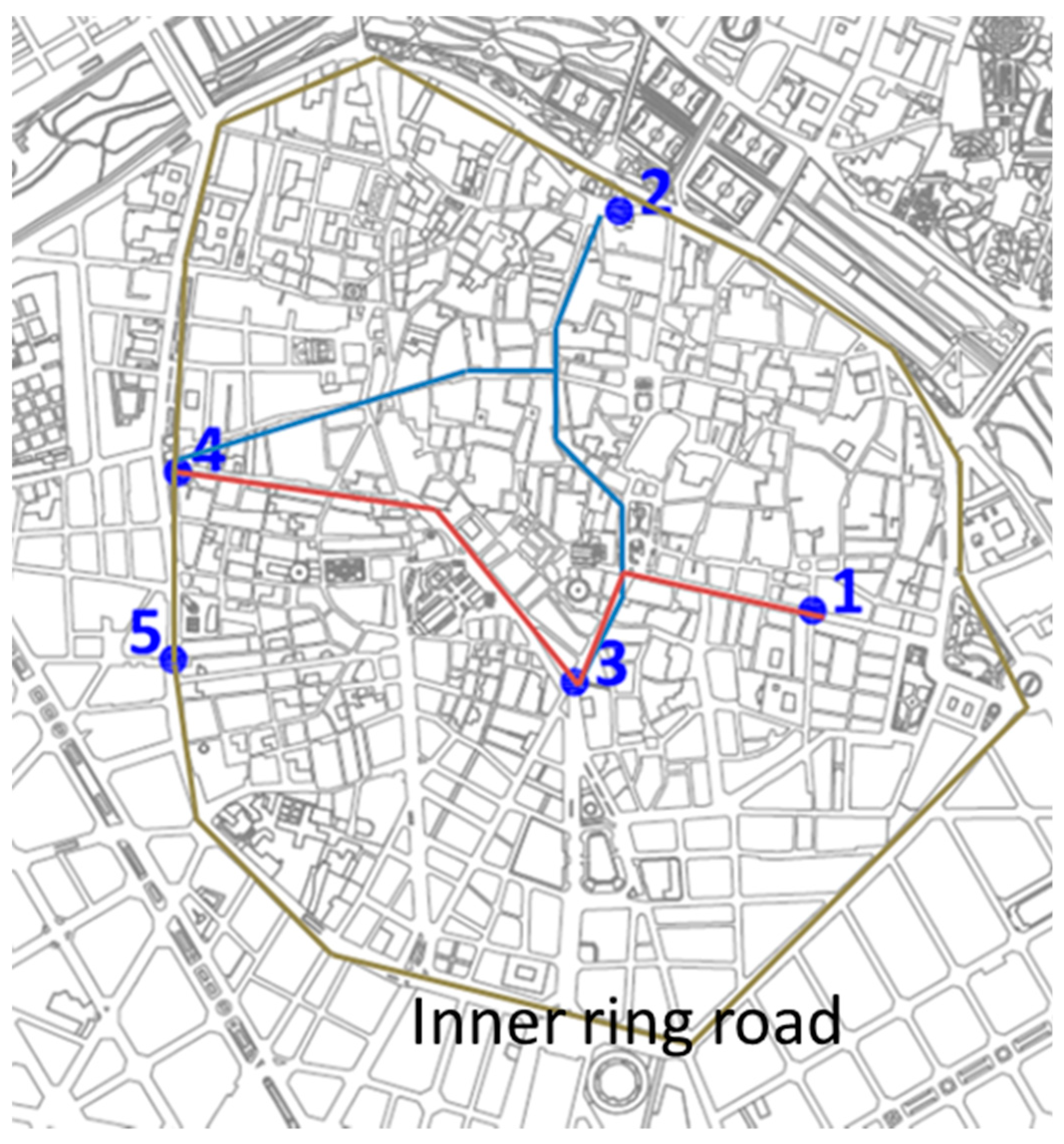
4.2. Definition of the Itineraries
- Route 1–3: La Paz - Comedias with San Vicente - Maria Cristina, distance 500 m.
- Route 3–4: San Vicente - Maria Cristina with Torres de Quart, distance 800 m.
- Route 2–3: Conde Trénor with San Vicente - Maria Cristina, distance 1000 m.
- Route 2–4: Conde Trénor with Torres de Quart, distance 1100 m.
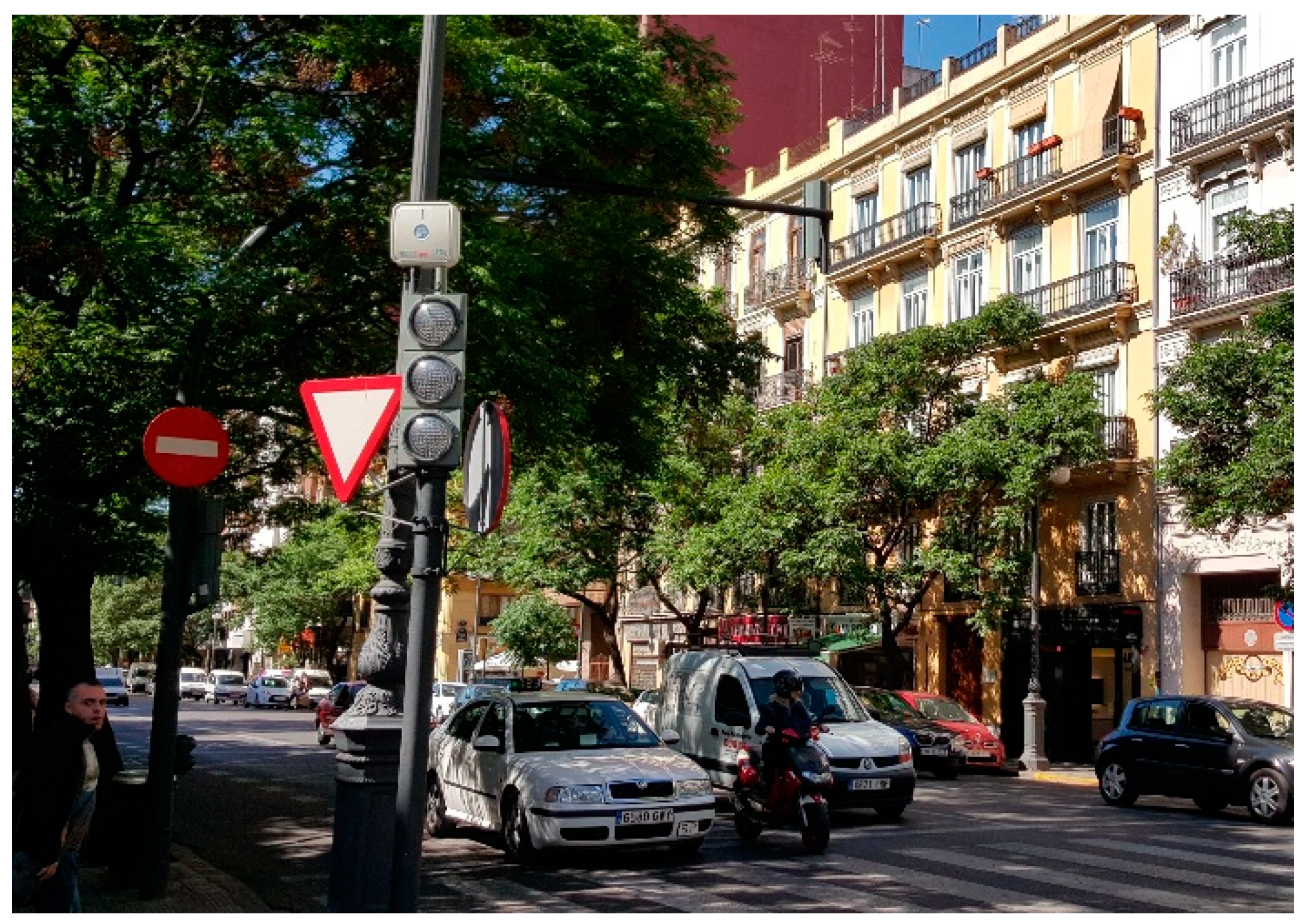
4.3. Location of Sensors
- Location 1: Paz - Comedias, entry sensor, allows the detection of the vehicles that enter the historic center and follow route 1–3.
- Location 2: Conde Trénor, entry sensor, allows the detection of the vehicles that enter the historic center and follow route 2–3 or 2–4.
- Location 3: San Vicente between Plaza de la Reina and Plaza del Ayuntamiento, exit sensor, allows the detection of the vehicles that leave the historic center in route 1–3 or 2–3.
- Location 4: Quart-Murillo, exit sensor, allows the detection of the vehicles that leave the historic center in route 2–4 or 3–4.
- Location 5: Guillem de Castro - Lepanto, intermediate sensor, detects vehicles that have been registered at the entry of Conde de Trénor, but have not entered the city center, they have followed the internal ring road. These vehicles were detected by the rear lobe of the antenna. Devices that followed itinerary 2–5–4 were disregarded in the current study because they do not use the historic center.
4.4. Description of the Study
- Establishing the location of the sensors, trying to minimize the power cabling, being careful that there would be no obstacles between the sensor and the vehicles and making sure it covered a wide area of the street to improve the detection of the devices.
- Installation and configuration of the equipment.
- Controlled tests with known BT devices to determine the classification algorithm for pedestrians and motor vehicles.
- Removal of equipment and collection of sensor data.
- Filtering the data of each sensor and creating the detection intervals. All detections of the same device are grouped in each sensor while it remains in the detection area. The intervals created coincide with the times the device passes through the detection area.
- Creation of trips between sensors.
- Application of the classification algorithm for the trips to separate vehicles from pedestrians.
- Calculation of the travel time and classification of the trips according to the criteria established in the study. Trips that do not stop on the route and use the itinerary to shorten the route through the city and trips that have as origin or destination some point of the historic center of Valencia
- Presentation of the results and conclusions.
5. Results of the Study
5.1. Classification Algorithm for Vehicles and Pedestrians
5.2. Detection Rate
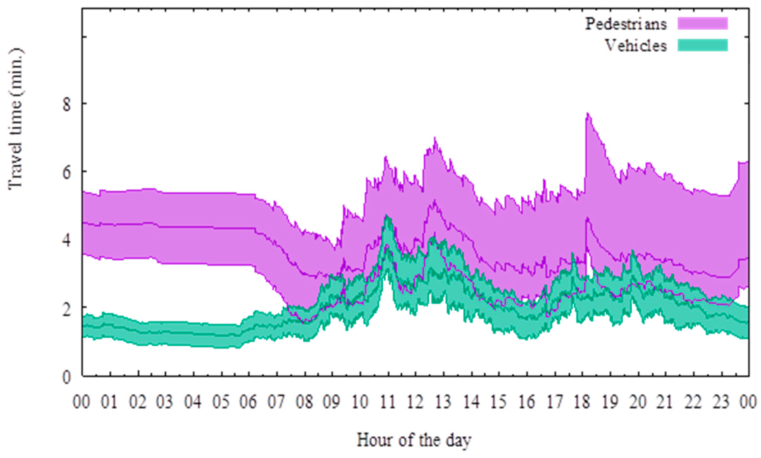
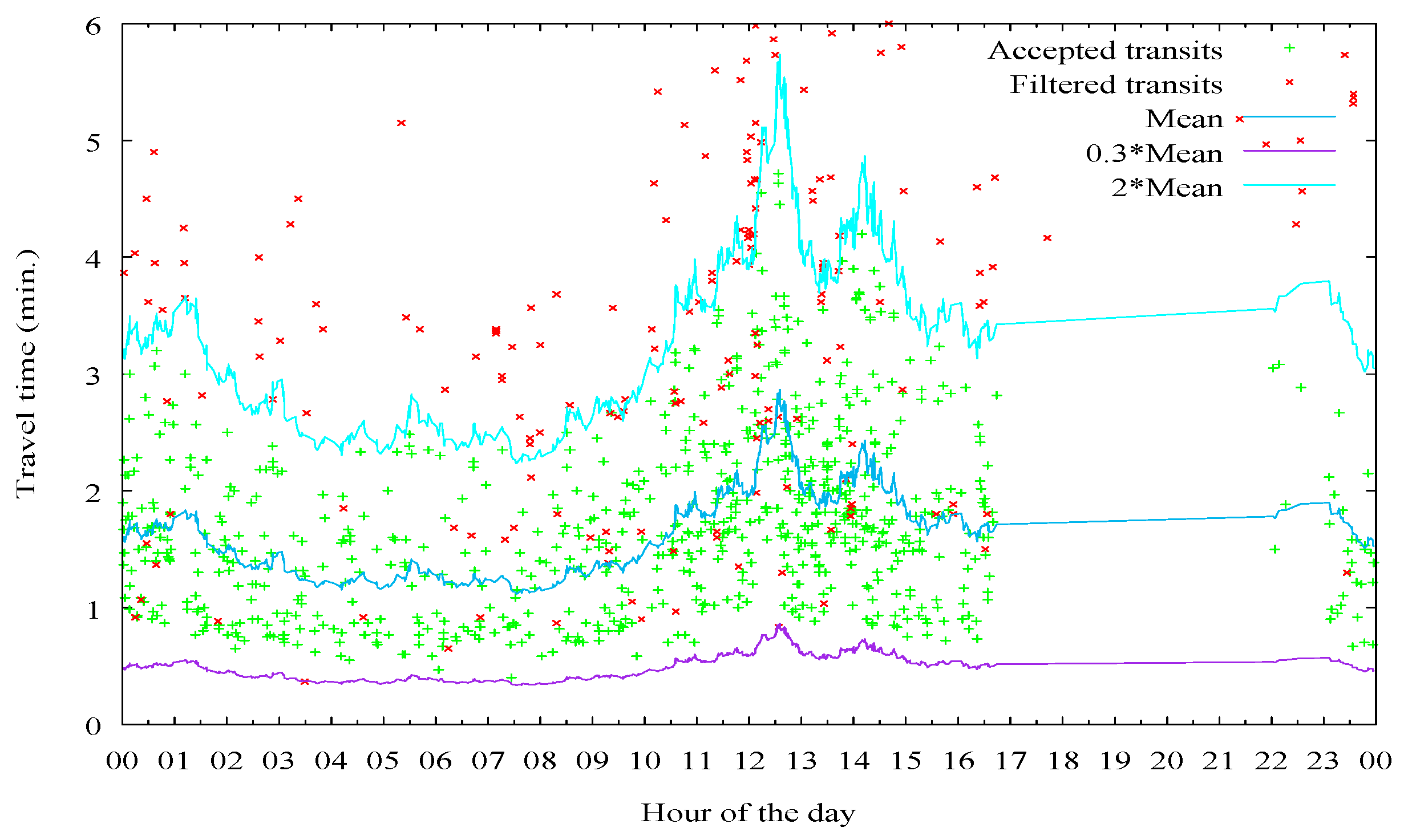
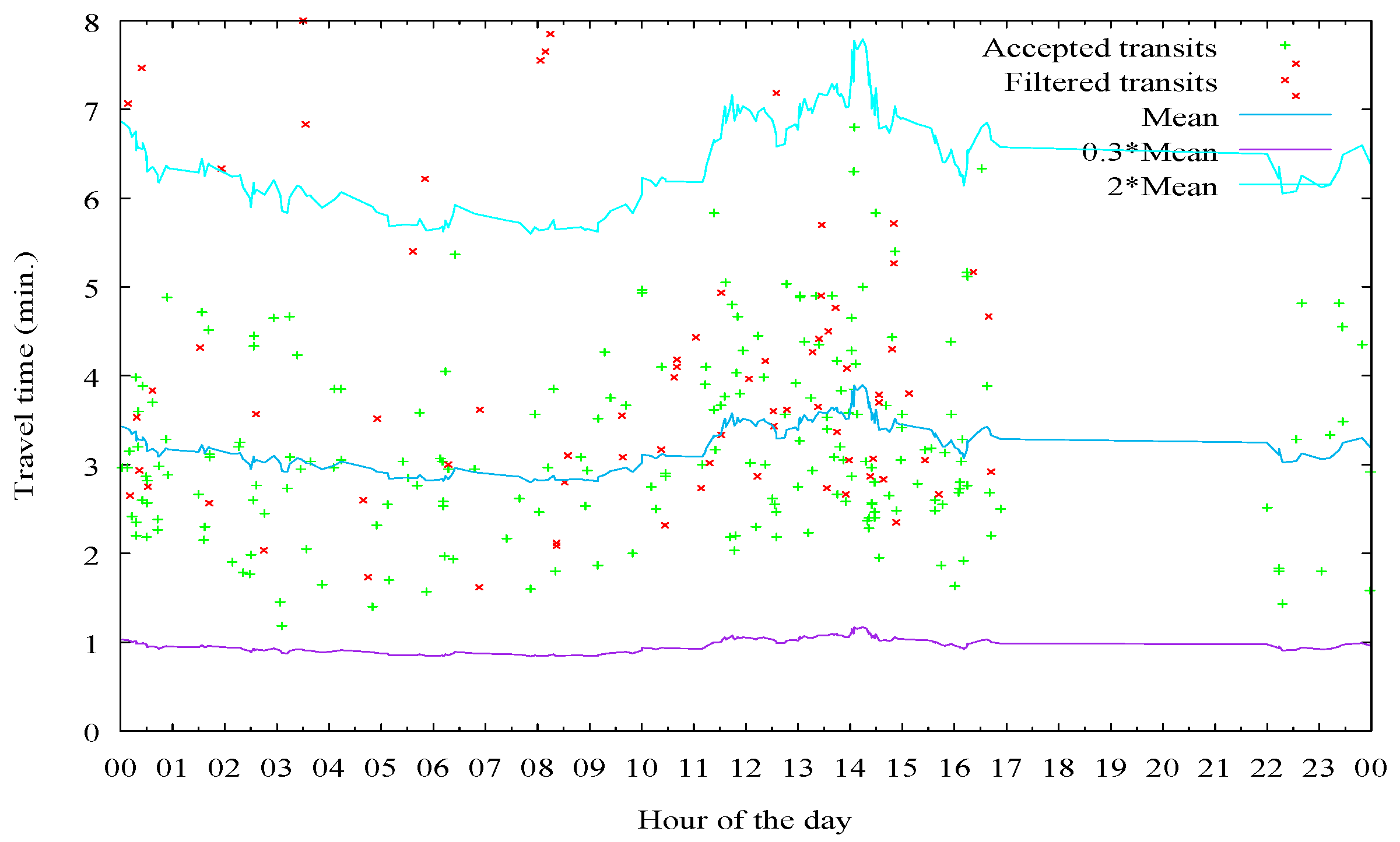
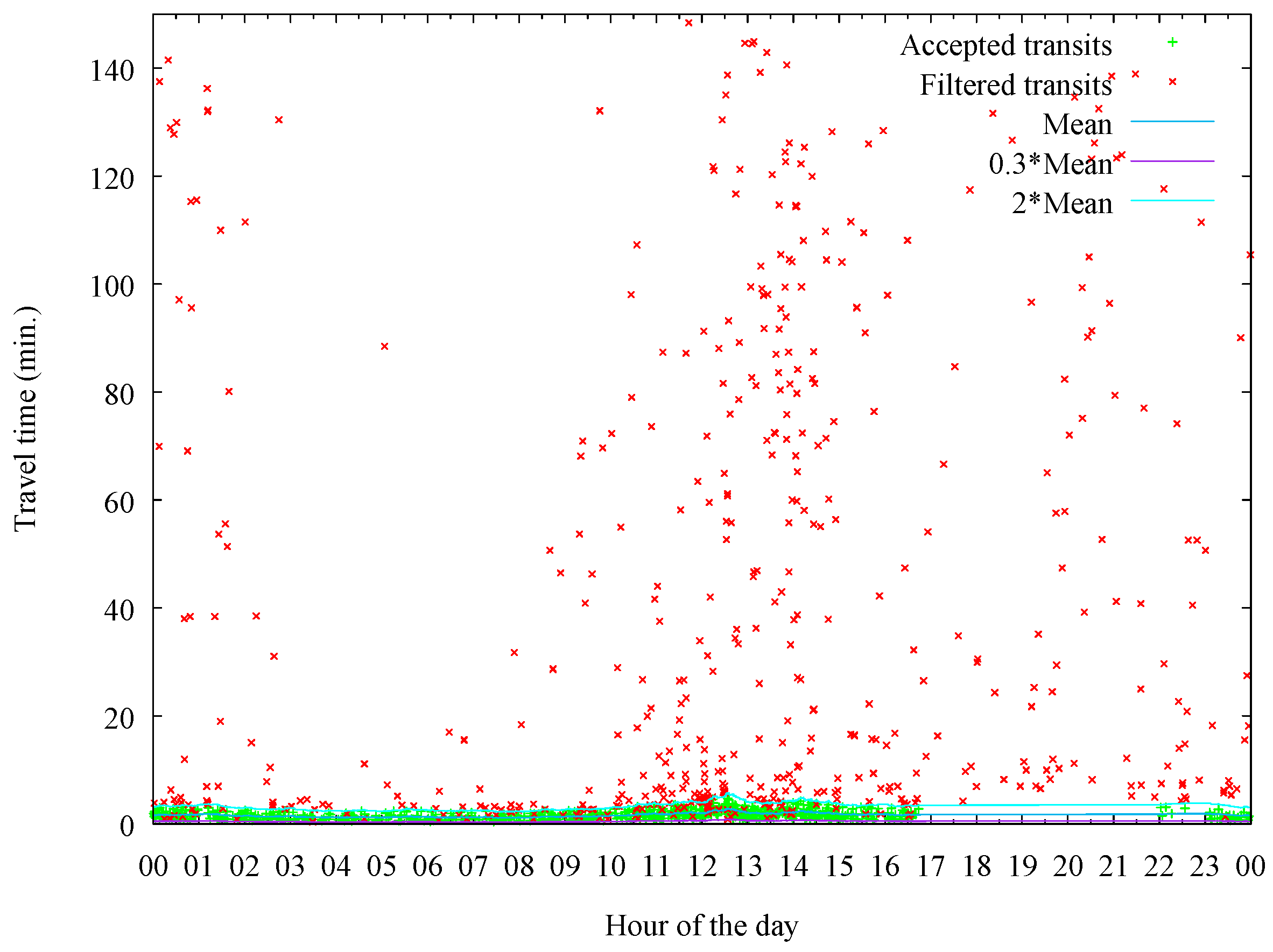
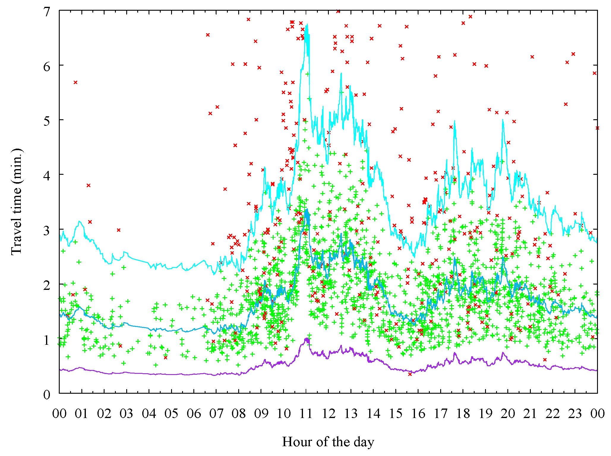
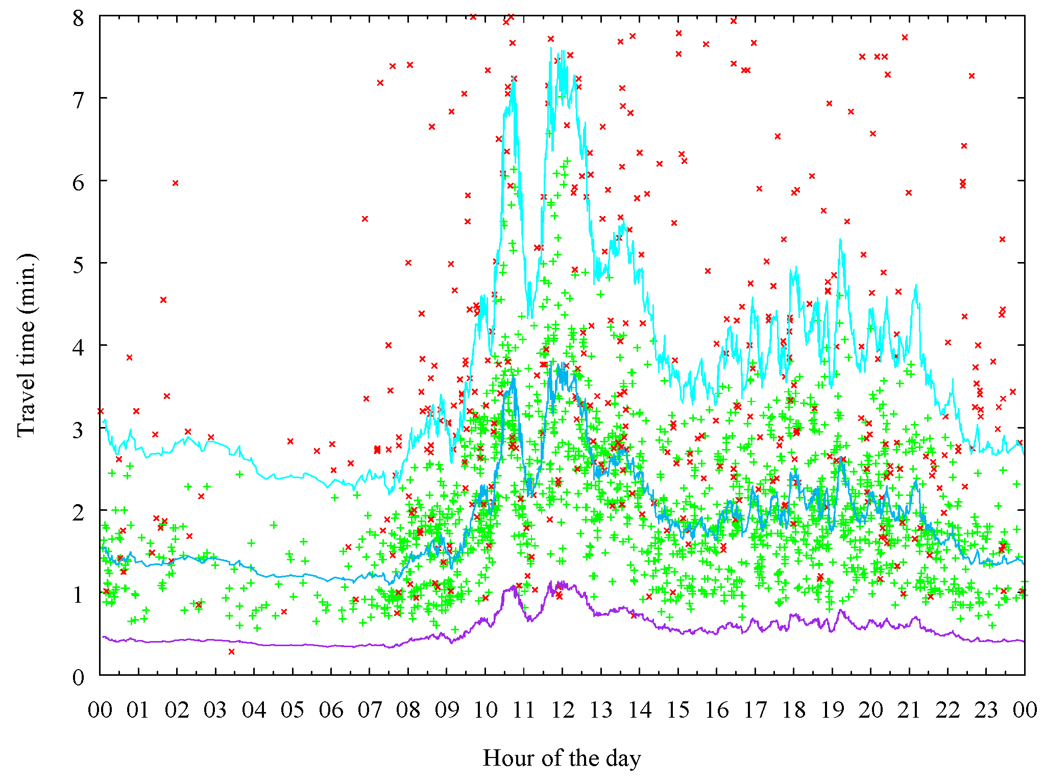
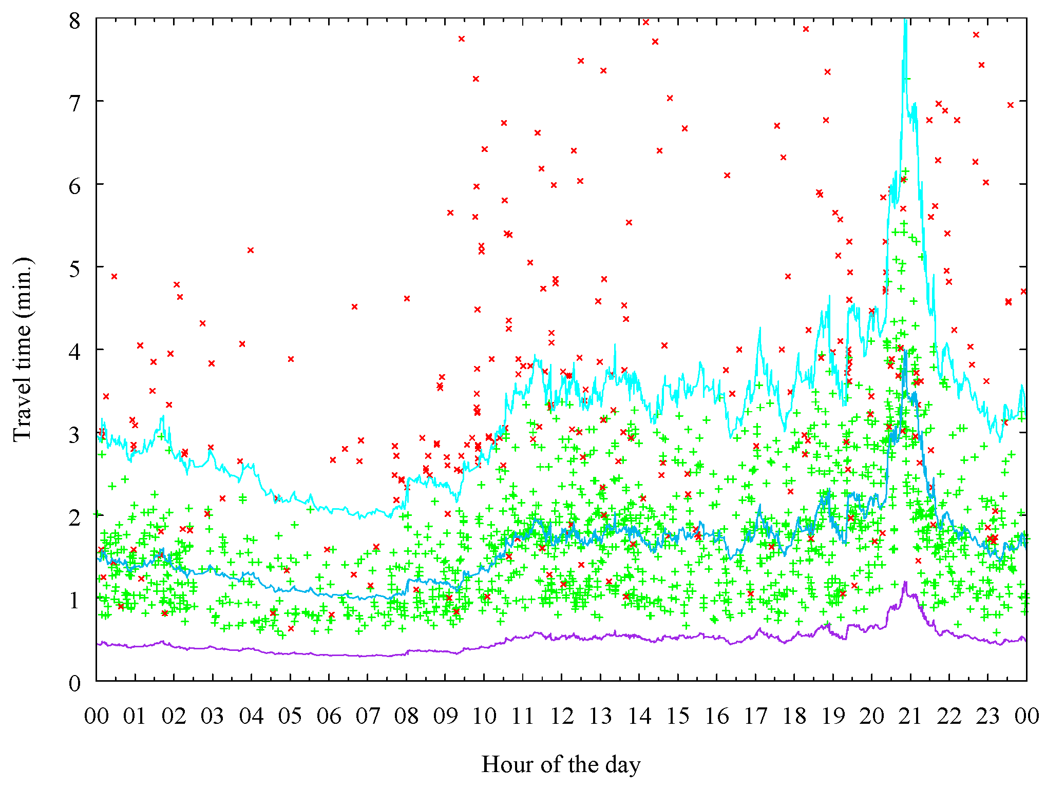
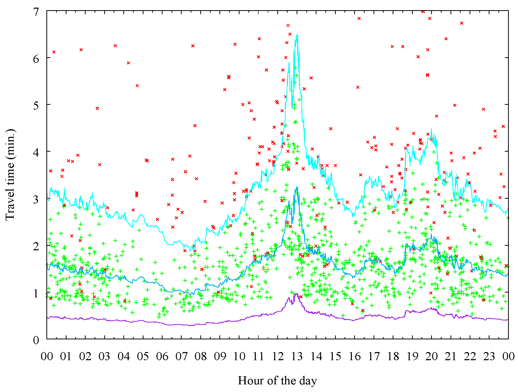
5.3. Travel Time
| algorithm |
| = |
| if (()) |
| end_if |
| end_algorithm |
- (0): Initial travel time between sensors i - j.
- : Travel time associated with the free flow speed between sensors i - j.
- (p): Average travel time at instant p between sensors i - j.
- (p): Calculated travel time of trip k between sensors i - j at temporal instant p.
- sup: Constant, in this study it takes value 2, sets the travel time value from which it is considered that the vehicle has made arrangements between the sensors (vehicle circulates two times slower than the average travel time).
- inf: Constant, in this study it takes value 0.3, it sets the travel time value from which a lower value would be a non-real data (vehicle circulates three times faster than the average travel time).
- β: Constant value that allows setting the value of taking into account the travel time value of the new valid trip registered. Typical values between 0.03 and 0.05
- : Trips classified as valid, value of the O/D matrix in the route, in the temporal interval p.
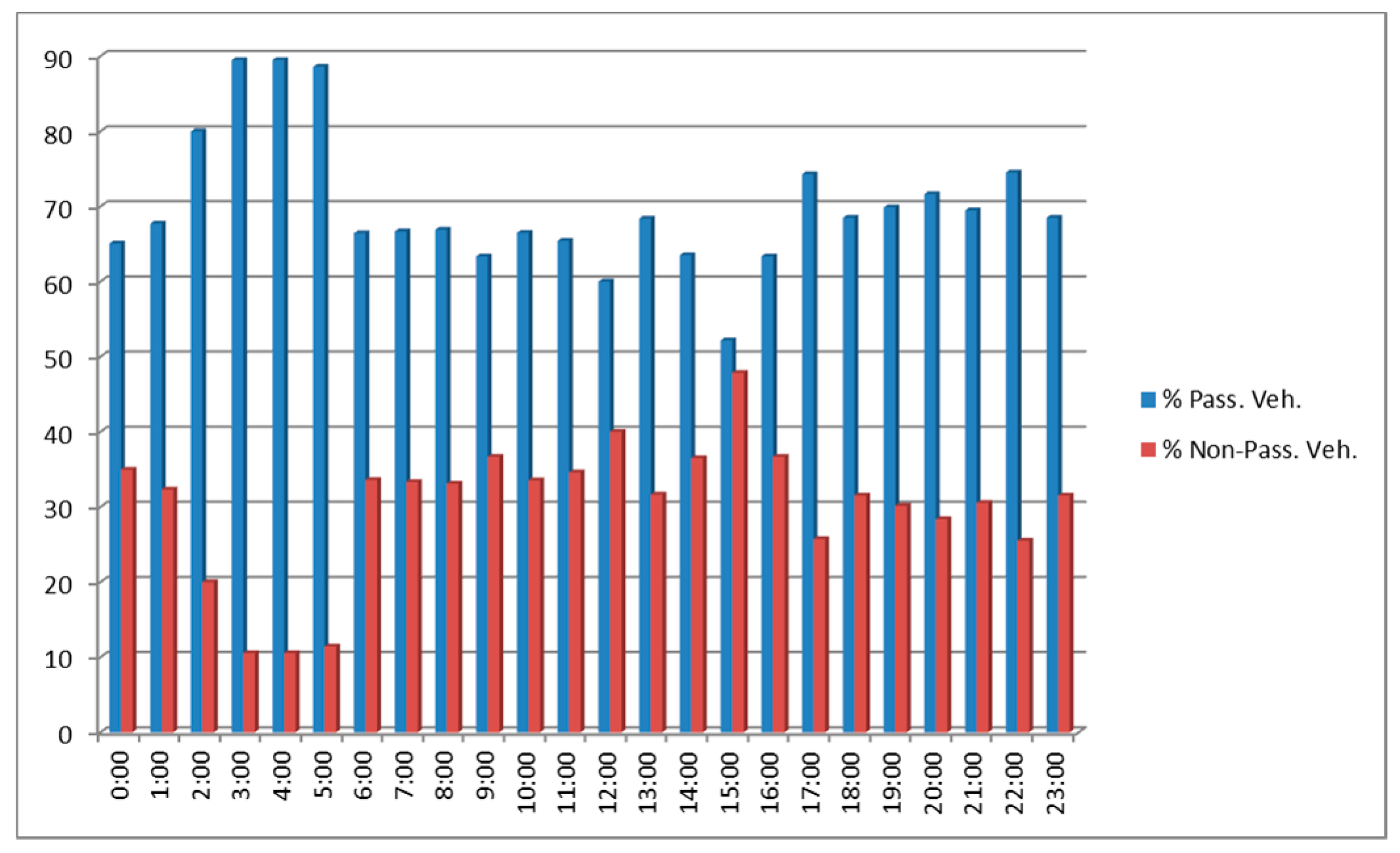
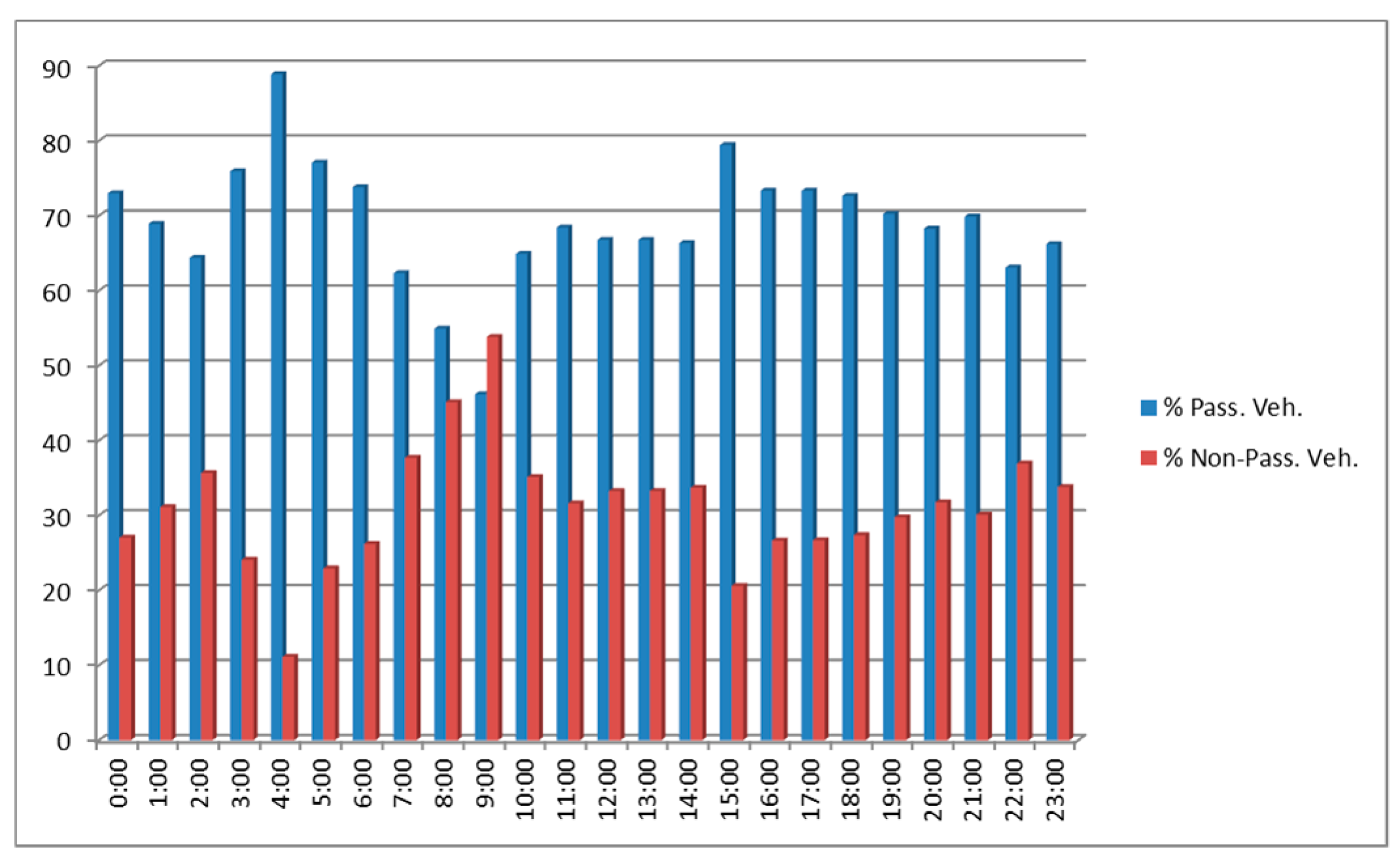
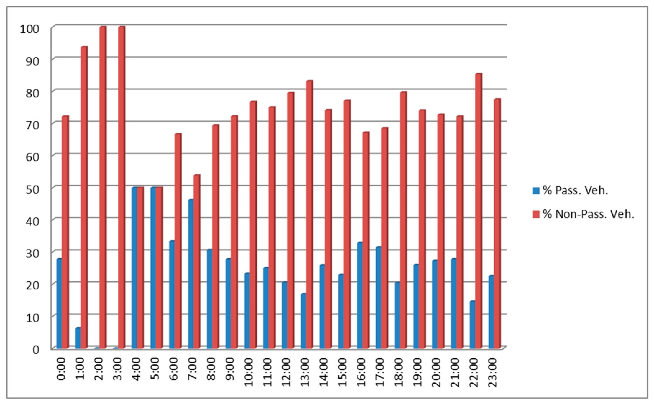
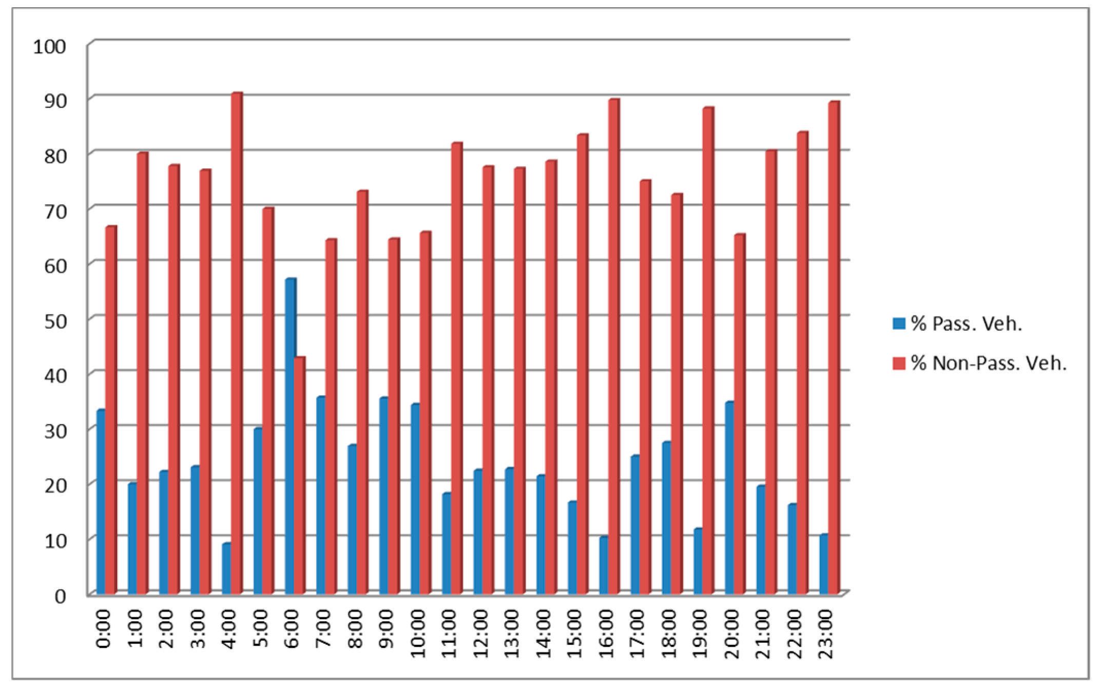
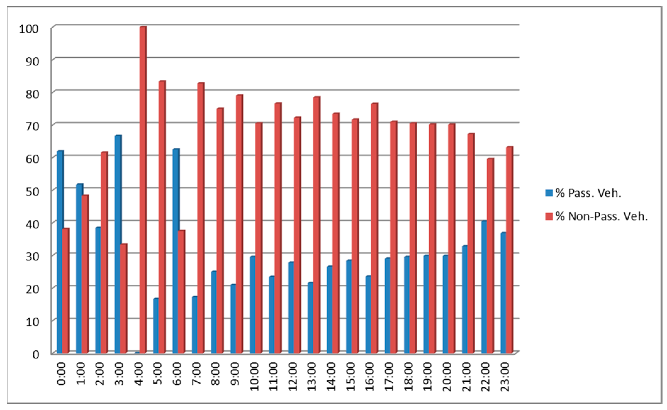
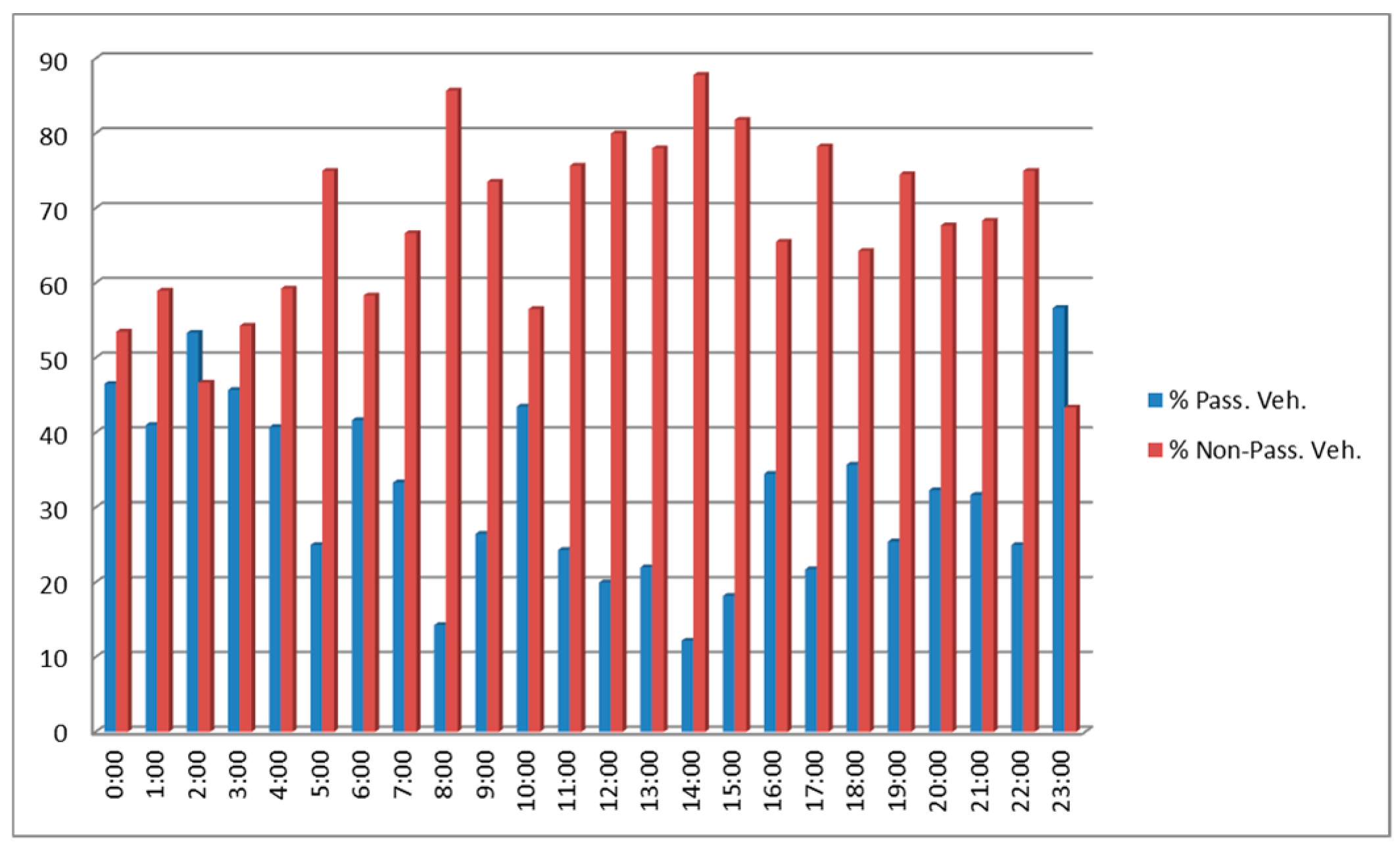
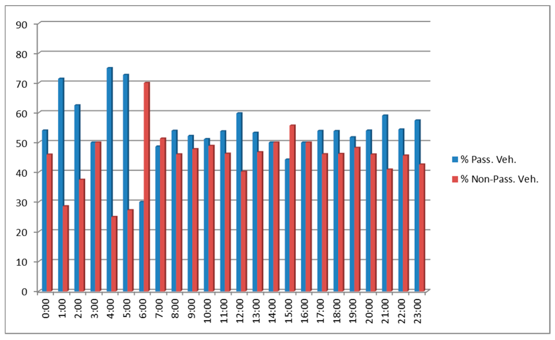
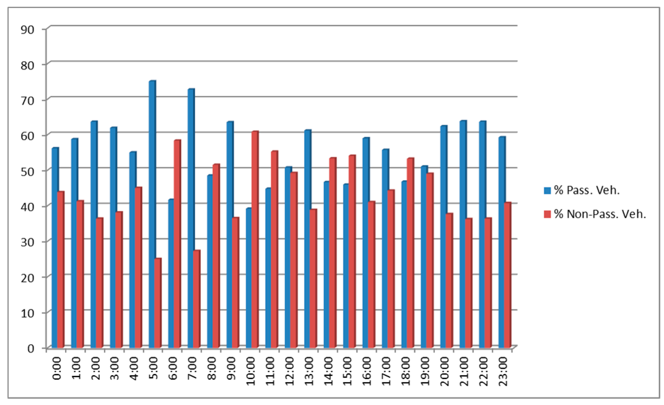
5.4. Percentages of Travel Distribution
6. Conclusions
Author Contributions
Funding
Acknowledgments
Conflicts of Interest
References
- Abrahamsson, T. Estimation of Origin-Destination Matrices Using Traffic Counts—A Literature Survey; IIASA: Laxenburg, Austria, 1998. [Google Scholar]
- Cascetta, E.; Postorino, M.N. Fixed Point Approaches to the Estimation of O/D Matrices Using Traffic Counts on Congested Networks. Transp. Sci. 2001, 35, 134–147. [Google Scholar] [CrossRef]
- Zhang, X.; Mustard, D. Methods for the estimation of time-dependent origin destination matrices using traffic flow data on road links. In Proceedings of the European Transport Conference, Cambridge, UK, 9–11 September 2002; p. 16. [Google Scholar]
- Hutchinson, E.; Hagen, L.; Pirinccioglu, F. Development of Revised Methodology for Collecting Origin-Destination Data; FDOT: Tampa, FL, USA, 2006. [Google Scholar]
- Sun, Y.; Zhu, H.; Zhou, X.; Sun, L. VAPA: Vehicle Activity Patterns Analysis based on Automatic Number Plate Recognition System Data. Procedia Comput. Sci. 2014, 31, 48–57. [Google Scholar] [CrossRef] [Green Version]
- Kwon, J.; Varaiya, P. Real-Time Estimation of Origin-Destination Matrices with Partial Trajectories from Electronic Toll Collection Tag Data. Transp. Res. Rec. J. Transp. Res. Board 2005, 1923, 119–126. [Google Scholar]
- Araghi, B.N.; Christensen, L.T.; Krishnan, R.; Lahrmann, H. Application of Bluetooth Technology for Mode- Specific Travel Time Estimation on Arterial Roads: Potentials and Challenges. In Proceedings of the Annual Transport Conference, Aalborg University, Aalborg, Denmark, 9–12 July 2012; pp. 1–15. [Google Scholar]
- Porter, J.D.; Kim, D.S.; Magana, M.E. Wireless Data Collection System for Real-Time Arterial Travel Time Estimates; Portland State University: Portland, OR, USA, 2011. [Google Scholar]
- Tornero, R.; Martínez, J.; Castelló, J. A multi-agent system for obtaining dynamic origin/destination matrices on intelligent road networks. In Proceedings of the 6th Euro American Conference on Telematics and Information Systems EATIS ’12, Valencia, Spain, 23–25 May 2012; p. 157. [Google Scholar]
- Michau, G.; Nantes, A.; Chung, E.; Abry, P. Retrieving dynamic origin-destination matrices from Bluetooth data. In Proceedings of the Transportation Research Board 93rd Annual Meeting, Washington, DC, USA, 12–16 January 2014; pp. 12–16. [Google Scholar]
- Malinovskiy, Y.; Lee, U.-K.; Wu, Y.-J.; Wang, Y. Investigation of Bluetooth-Based Travel Time Estimation Error on a Short Corridor. In Proceedings of the Transportation Research Board 90th Annual Meeting, Washington, DC, USA, 23–27 January 2011; p. 19. [Google Scholar]
- Wang, Y.; Malinovskiy, Y.; Wu, Y. Error Modeling and Analysis for Travel Time Data Obtained from Bluetooth MAC Address Matching; U.S. Department of Transportation: Washington, DC, USA, 2011.
- Stevanovic, A.; Olarte, C.L.; Galletebeitia, Á.; Galletebeitia, B.; Kaisar, E.I. Testing Accuracy and Reliability of MAC Readers to Measure Arterial Travel Times. Int. J. Intell. Transp. Syst. Res. 2015, 13, 50–62. [Google Scholar] [CrossRef]
- Bhaskar, A.; Chung, E. Fundamental understanding on the use of Bluetooth scanner as a complementary transport data. Transp. Res. Part C Emerg. Technol. 2013, 37, 42–72. [Google Scholar] [CrossRef] [Green Version]
- Blogg, M.; Semler, C.; Hingorani, M.; Troutbeck, R. Travel Time and Origin-Destination Data Collection Using Bluetooth MAC Address Readers; The National Academies of Sciences, Engineering, and Medicine: Washington, DC, USA, 2010; pp. 1–15. [Google Scholar]
- Barceló, J.; Montero, L.; Marqués, L.; Carmona, C. Travel Time Forecasting and Dynamic Origin-Destination Estimation for Freeways Based on Bluetooth Traffic Monitoring. Transp. Res. Rec. J. Transp. Res. Board 2010, 2175, 19–27. [Google Scholar] [CrossRef] [Green Version]
- Tsubota, T.; Bhaskar, A.; Chung, E.; Billot, R. Arterial traffic congestion analysis using Bluetooth Duration data. In Proceedings of the Australasian Transport Research Forum, Adelaide, SA, Australia, 28–30 September 2011; pp. 28–30. [Google Scholar]
- Day, C.; Wasson, J.; Brennan, T.; Bullock, D. Application of Travel Time Information for Traffic Management; Indiana Department of Transportation and Purdue University: West Lafayette, IN, USA, 2012. [Google Scholar]
- Laharotte, P.; Billot, R.; Come, E.; Oukhellou, L.; Nantes, A.; el Faouzi, N.-E. Spatiotemporal Analysis of Bluetooth Data: Application to a Large Urban Network. IEEE Trans. Intell. Transp. Syst. 2014, 16, 1–10. [Google Scholar] [CrossRef]
- Carpenter, C.; Fowler, M.; Adler, T. Generating Route-Specific Origin-Destination Tables Using Bluetooth Technology. Transp. Res. Rec. J. Transp. Res. Board 2012, 2308, 96–102. [Google Scholar] [CrossRef]
- Plumé, J.M.; Gimeno, R.V.C.; García, F.R.S. Influence of Percentage of Detection on Origin—Destination Matrices Calculation from Bluetooth and Wifi Mac Address Collection Devices. In Proceedings of the Industrial Simulation Conference 2015, Huntington Beach, CA, USA, 6–9 December 2015; pp. 108–112. [Google Scholar]
- Becker, R.A.; Caceres, R.; Hanson, K.; Loh, J.M.; Urbanek, S.; Varshavsky, A.; Volinsky, C.; Ave, P.; Park, F. Route Classification Using Cellular Handoff Patterns. In Proceedings of the 13th international conference on Ubiquitous computing, Beijing, China, 17–21 September 2011; pp. 123–132. [Google Scholar]
- Iqbal, S.; Choudhury, C.F.; Wang, P.; González, M.C. Development of origin—Destination matrices using mobile phone call data. Transp. Res. Part C 2014, 40, 63–74. [Google Scholar] [CrossRef]
- Puckett, D.D.; Vickich, M.J. Bluetooth ®-Based Travel Time/Speed Measuring Systems Development Final Report; Texas Transportation Institute: Austin, TX, USA, 2010; UTCM 09-00-17. [Google Scholar]
- Malinovskiy, Y.; Saunier, N.; Wang, Y. Pedestrian Travel Analysis Using Static Bluetooth Sensors. In Proceedings of the 91st Annual Transportation Research Board Meeting, Washington, DC, USA, 22–26 January 2012. [Google Scholar]
- Versichele, M.; Neutens, T.; Delafontaine, M.; Van de Weghe, N. The use of Bluetooth for analysing spatiotemporal dynamics of human movement at mass events: A case study of the Ghent Festivities. Appl. Geogr. 2012, 32, 208–220. [Google Scholar] [CrossRef] [Green Version]


| Transport Mode | Mean of Number of Detections | Typical Deviation |
|---|---|---|
| Pedestrian | 80.1 | 16 |
| Car | 8.3 | 8.5 |
| Both | 16.1 | 17.1 |
| MAC | Device | Number of Trips | Classified as Vehicle | Classified as Pedestrian |
|---|---|---|---|---|
| 00:21:3E:XX:XX:XX | TomTom | 763 | 743 | 20 |
| 00:26:7E:XX:XX:XX | Parrot | 752 | 736 | 16 |
| Date | Daily Traffic (loop) | Filtered Detections | Total Detections | Filtered Detections (%) | Total Detections (%) |
|---|---|---|---|---|---|
| 28-may | 16,282 | 2089 | 6920 | 12.83 | 42.50 |
| 29-may | 16,885 | 2104 | 6838 | 12.46 | 40.50 |
| 30-may | 13,606 | 1680 | 5255 | 12.35 | 38.62 |
| 31-may | 9861 | 1187 | 4011 | 12.04 | 40.68 |
| 01-jun | 16,069 | 1987 | 6374 | 12.37 | 39.67 |
| 02-jun | 15,495 | 1929 | 6414 | 12.45 | 41.39 |
| 03-jun | 15,876 | 2107 | 6643 | 13.27 | 41.84 |
| 04-jun | 17,222 | 2105 | 7077 | 12.22 | 41.09 |
| 05-jun | 17,302 | 2193 | 6986 | 12.67 | 40.38 |
| 06-jun | 13,496 | 1642 | 5372 | 12.17 | 39.80 |
| 07-jun | 10,338 | 960 | 4425 | 9.29 | 42.80 |
| 08-jun | 15,021 | 1907 | 6439 | 12.70 | 42.87 |
| Mean | 12.23 | 41.01 | |||
| Typical Deviation | 0.99 | 1.33 |
| Route | Number of Trips | Passing | Non Passing |
|---|---|---|---|
| 1–3 | 43,713 | 68.5 | 31.5 |
| 2–4 | 12,076 | 24.5 | 75.5 |
| 2–3 | 8413 | 27.8 | 72.2 |
| 3–4 | 11,733 | 54.9 | 45.1 |
© 2019 by the authors. Licensee MDPI, Basel, Switzerland. This article is an open access article distributed under the terms and conditions of the Creative Commons Attribution (CC BY) license (http://creativecommons.org/licenses/by/4.0/).
Share and Cite
Martínez Plumé, J.; Marténez Durá, J.J.; Cirilo Gimeno, R.V.; Soriano García, F.R.; García Celda, A. Evaluation of the Use of a City Center through the Use of Bluetooth Sensors Network. Sustainability 2019, 11, 1002. https://0-doi-org.brum.beds.ac.uk/10.3390/su11041002
Martínez Plumé J, Marténez Durá JJ, Cirilo Gimeno RV, Soriano García FR, García Celda A. Evaluation of the Use of a City Center through the Use of Bluetooth Sensors Network. Sustainability. 2019; 11(4):1002. https://0-doi-org.brum.beds.ac.uk/10.3390/su11041002
Chicago/Turabian StyleMartínez Plumé, Javier, Juan José Marténez Durá, Ramón Vicente Cirilo Gimeno, Francisco Ramón Soriano García, and Antonio García Celda. 2019. "Evaluation of the Use of a City Center through the Use of Bluetooth Sensors Network" Sustainability 11, no. 4: 1002. https://0-doi-org.brum.beds.ac.uk/10.3390/su11041002