Assessing the Performance of UAS-Compatible Multispectral and Hyperspectral Sensors for Soil Organic Carbon Prediction

 , , and
Abstract
:1. Introduction
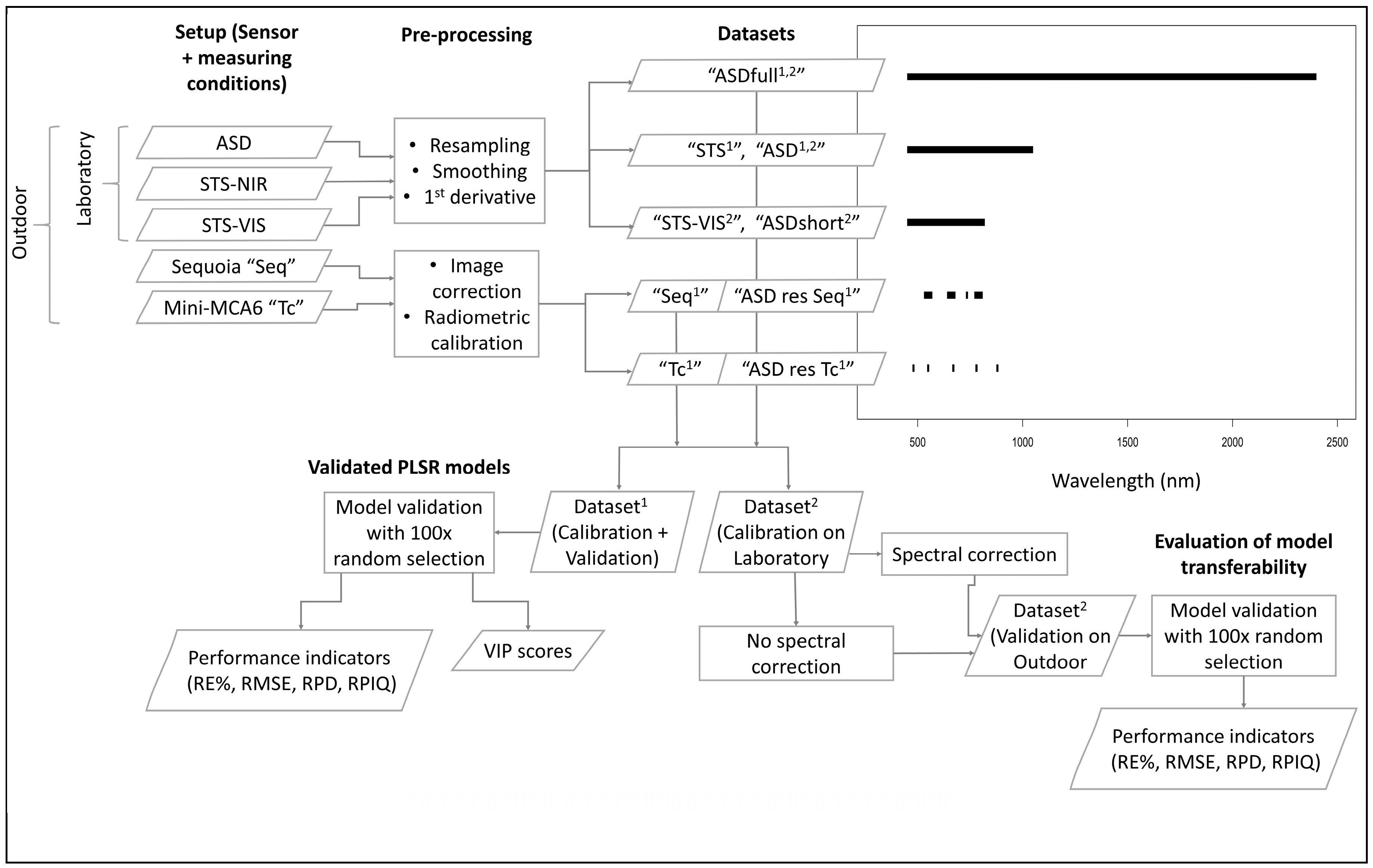
2. Materials and Methods
2.1. Soil Datasets
2.2. Sensor Equipment
2.3. Spectral Measurements
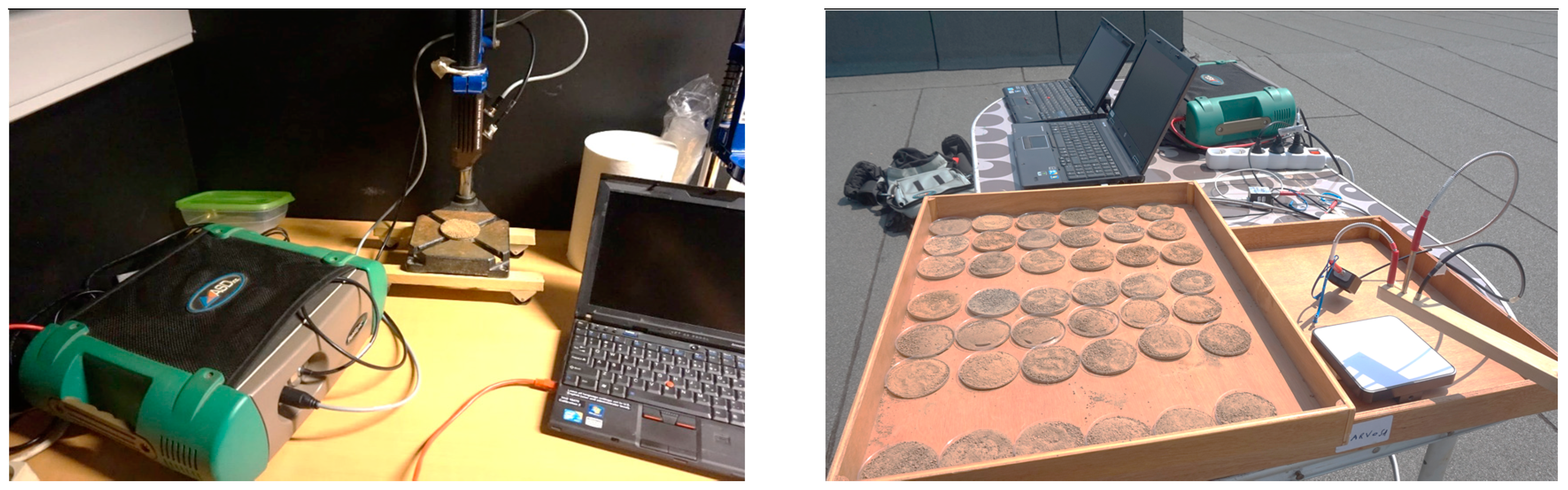
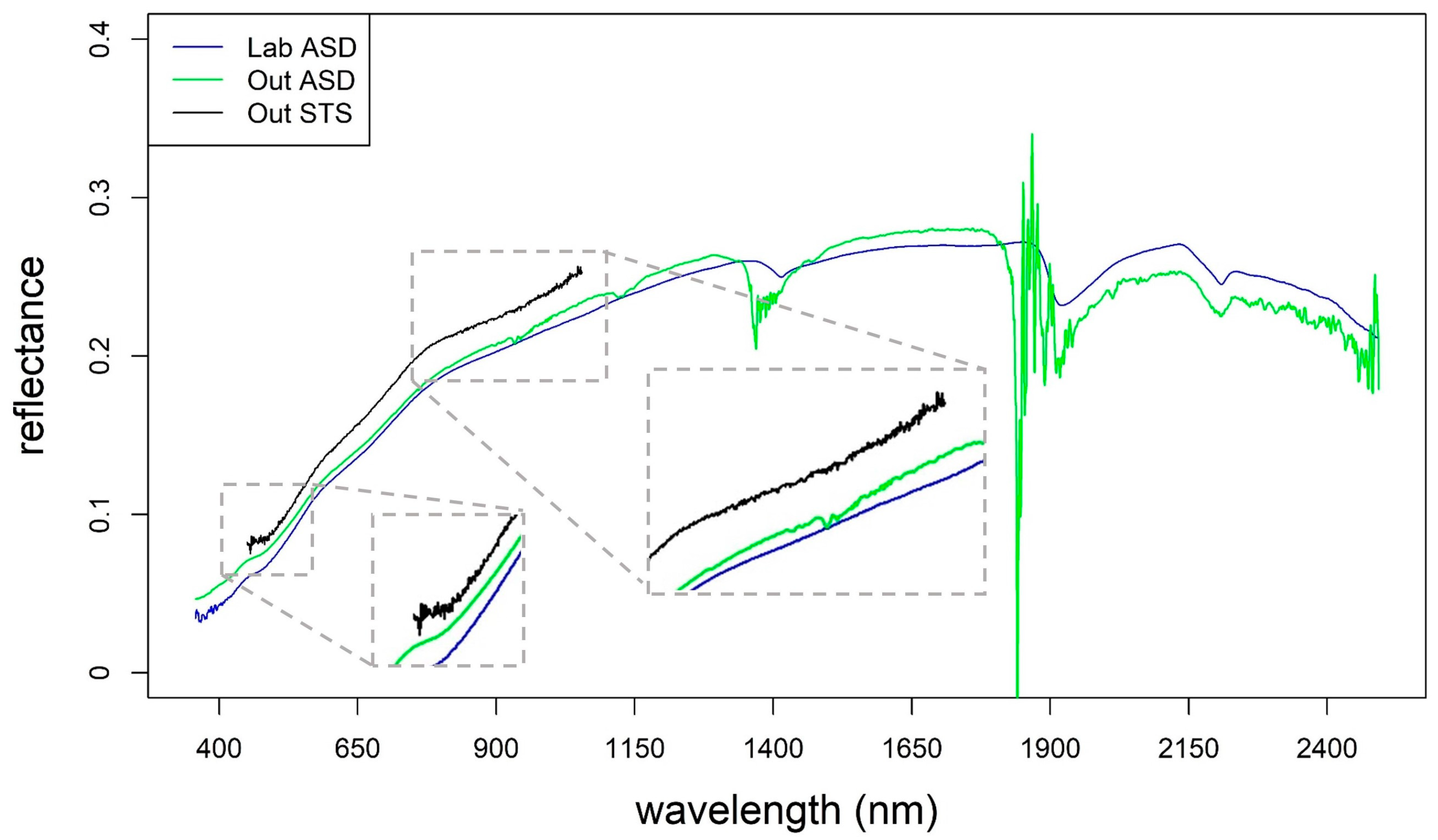
- Laboratory setup (“Lab” dataset): all samples were scanned once, by the ASD and the STS sensors, using the ASD contact probe, which is equipped with its own light source (100 W halogen reflectorized lamp), and that allows for a spot size of 10 mm of diameter. Measures were carried out with the probe in contact with the soil sample, in a dark room to minimize sources of disturbance (Figure 2, left).
- Outdoor setup (“Out” dataset): all samples were scanned once, in an open area, to minimize reflection from vertical objects in the surroundings, with stable, clear-sky, natural sunlight conditions for the whole duration of the measurements. In the ASD and STS cases, the sensor head was set at a 10 cm height above the samples, at the nadir position, providing a measuring spot size of 4.4 cm of diameter (Figure 2, right). In the cameras cases, the pictures were taken from a low altitude (c. 2 m) in the nadir position above the samples, resulting in c. [0–9]{1,}–[0–9]{1,} pixels/sample.
2.4. Comparison between Measurement Setups
2.5. Model Transferability between Measurement Setups
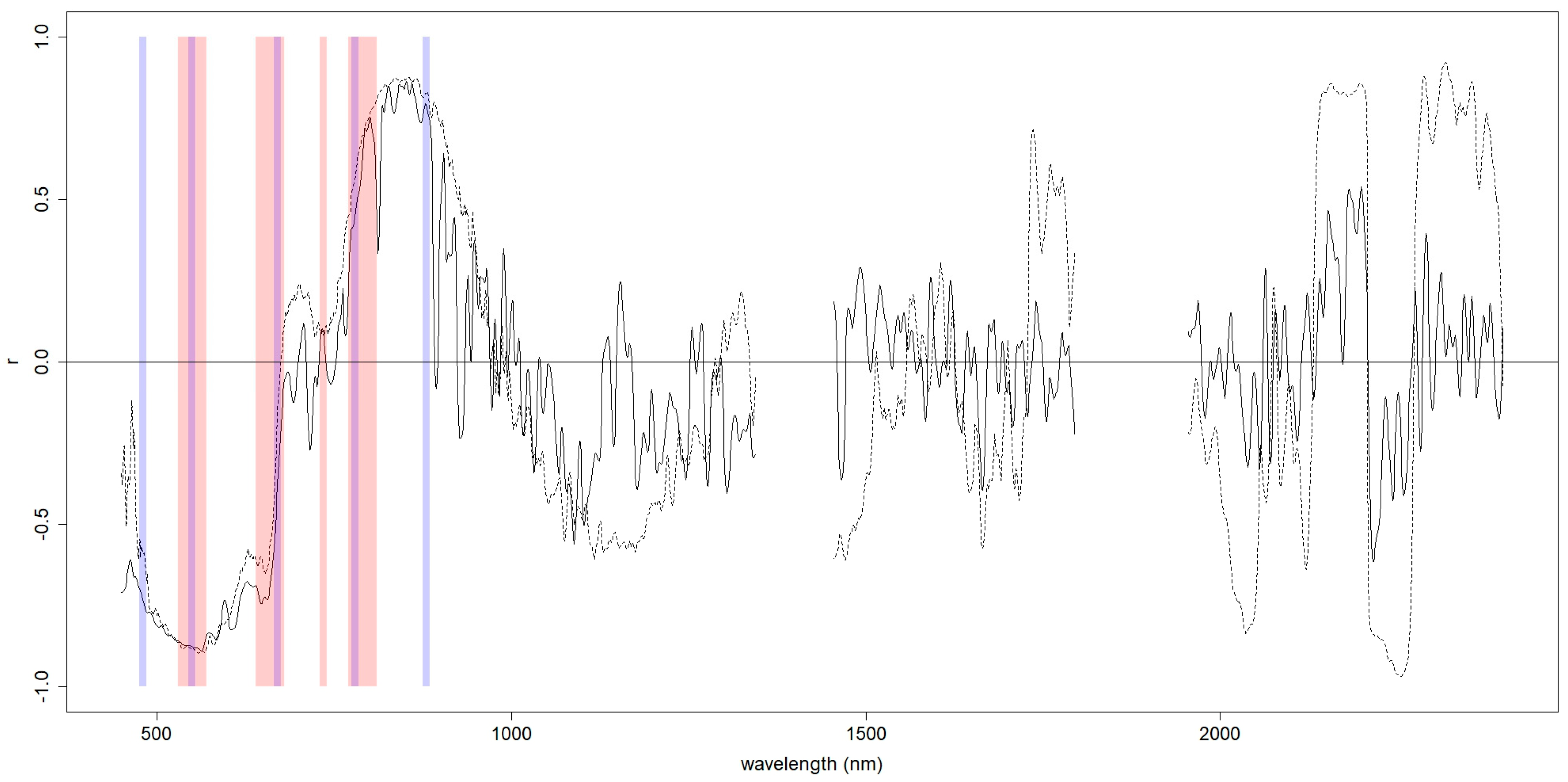
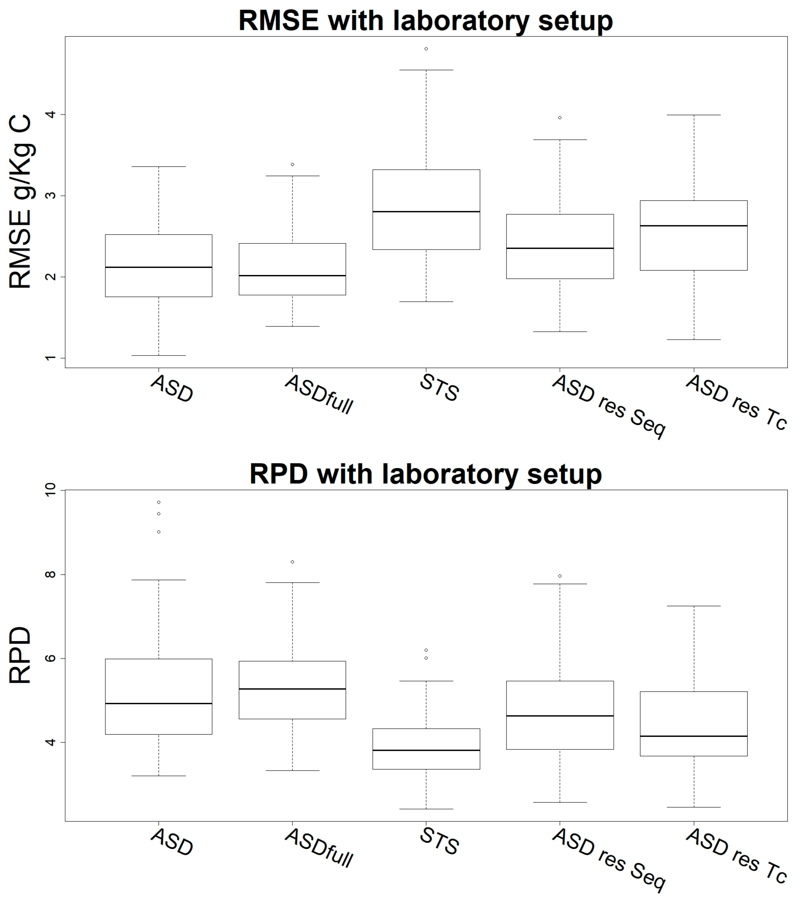
3. Results
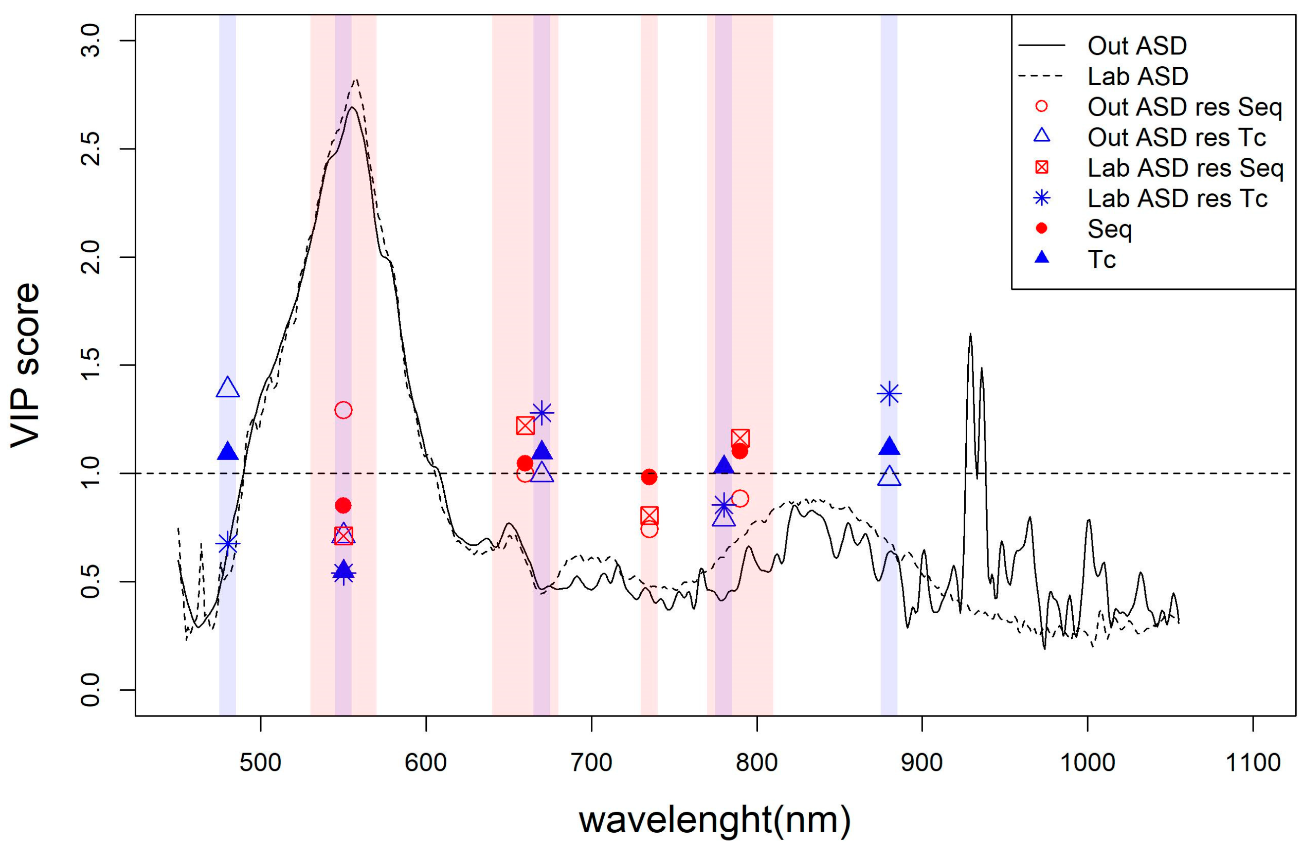
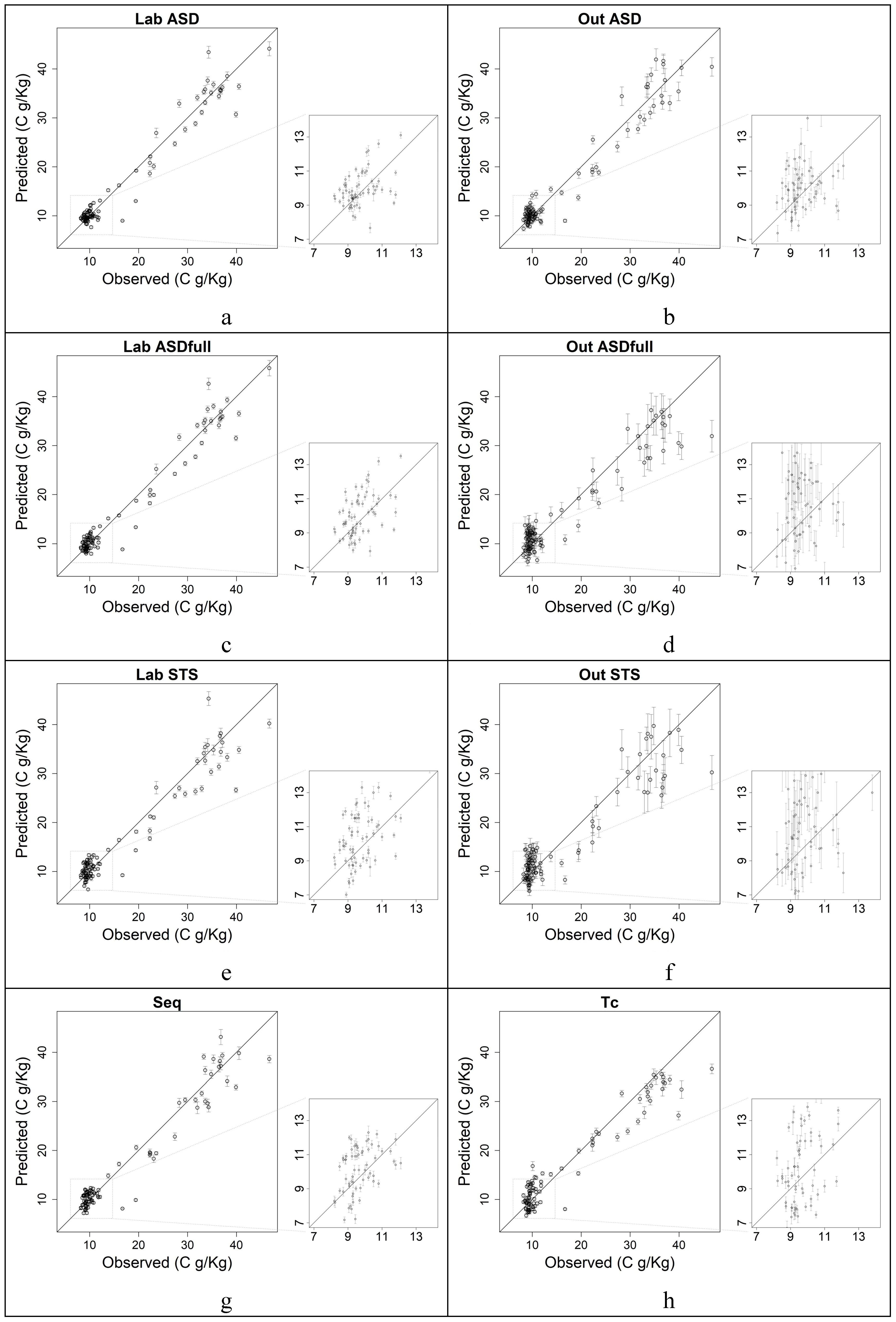
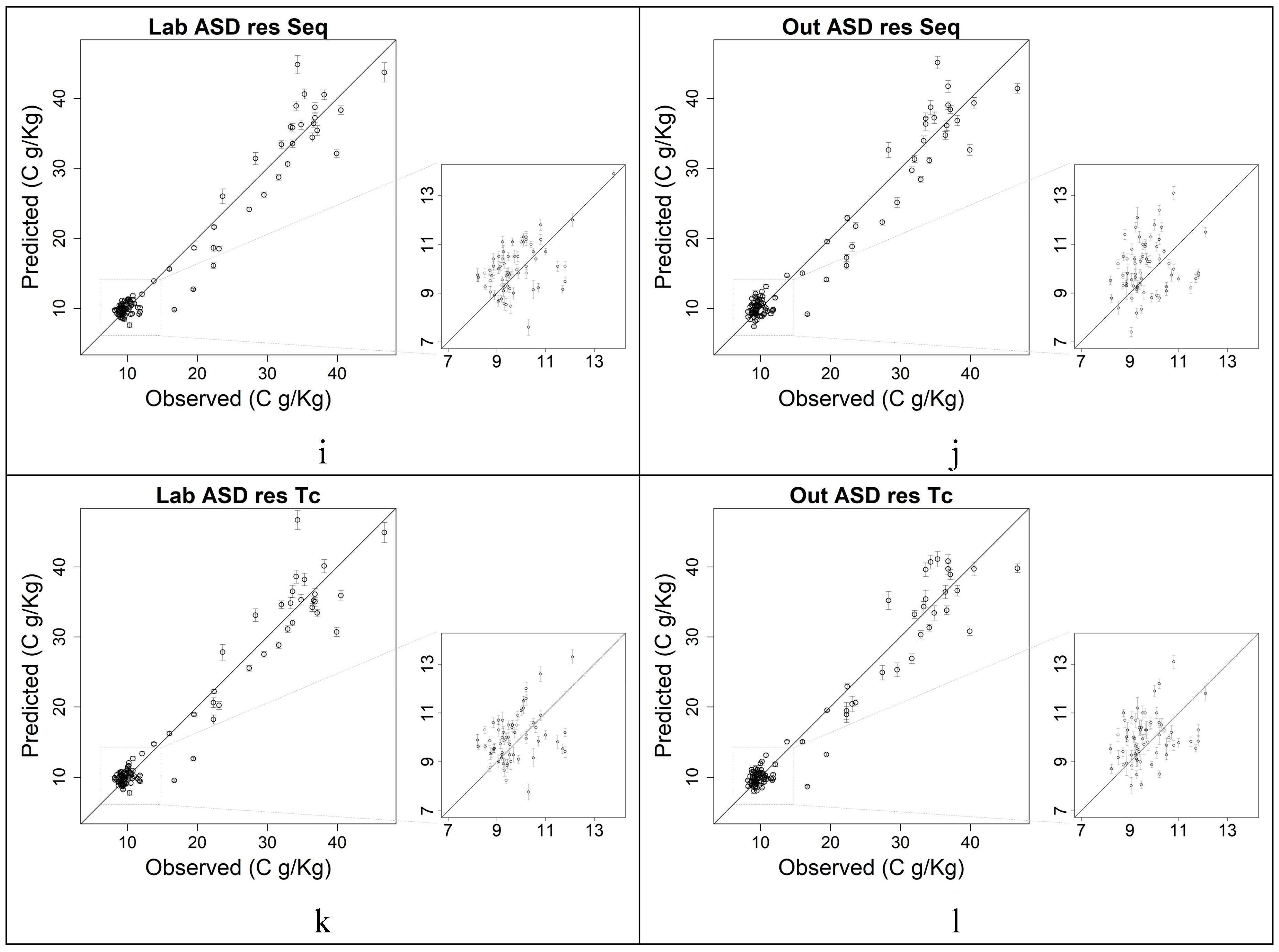
3.1. Validated PLSR Models
3.2. Evaluation of Model Transferability
4. Discussion
5. Conclusions
Author Contributions
Funding
Acknowledgments
Conflicts of Interest
Appendix A


References
- Nocita, M.; Stevens, A.; van Wesemael, B.; Aitkenhead, M.; Bachmann, M.; Barthès, B.; Ben Dor, E.; Brown, D.J.; Clairotte, M.; Csorba, A.; et al. Soil Spectroscopy: An Alternative to Wet Chemistry for Soil Monitoring. Adv. Agron. 2015, 132, 139–159. [Google Scholar] [CrossRef]
- Mouazen, A.M.; Maleki, M.R.; De Baerdemaeker, J.; Ramon, H. On-line measurement of some selected soil properties using a VIS-NIR sensor. Soil Tillage Res. 2007, 93, 13–27. [Google Scholar] [CrossRef]
- Stenberg, B.; Viscarra Rossel, R.A.; Mouazen, A.M.; Wetterlind, J. Visible and Near Infrared Spectroscopy in Soil Science. In Advances in Agronomy; Academic Press: Cambridge, MA, USA, 2010; Volume 107, pp. 163–215. [Google Scholar]
- Castaldi, F.; Palombo, A.; Santini, F.; Pascucci, S.; Pignatti, S.; Casa, R. Evaluation of the potential of the current and forthcoming multispectral and hyperspectral imagers to estimate soil texture and organic carbon. Remote Sens. Environ. 2016, 179, 54–65. [Google Scholar] [CrossRef]
- Nawar, S.; Mouazen, A.M. Predictive performance of mobile vis-near infrared spectroscopy for key soil properties at different geographical scales by using spiking and data mining techniques. Catena 2017, 151, 118–129. [Google Scholar] [CrossRef]
- Melendez-Pastor, I.; Navarro-Pedreño, J.; Gómez, I.; Koch, M. Identifying optimal spectral bands to assess soil properties with VNIR radiometry in semi-arid soils. Geoderma 2008, 147, 126–132. [Google Scholar] [CrossRef]
- Stevens, A.; Udelhoven, T.; Denis, A.; Tychon, B.; Lioy, R.; Hoffmann, L.; van Wesemael, B. Measuring soil organic carbon in croplands at regional scale using airborne imaging spectroscopy. Geoderma 2010, 158, 32–45. [Google Scholar] [CrossRef] [Green Version]
- Castaldi, F.; Casa, R.; Castrignanò, A.; Pascucci, S.; Palombo, A.; Pignatti, S. Estimation of soil properties at the field scale from satellite data: A comparison between spatial and non-spatial techniques. Eur. J. Soil Sci. 2014, 65, 842–851. [Google Scholar] [CrossRef]
- Castaldi, F.; Hueni, A.; Chabrillat, S.; Ward, K.; Buttafuoco, G.; Bomans, B.; Vreys, K.; Brell, M.; Wesemael, B. Van ISPRS Journal of Photogrammetry and Remote Sensing Evaluating the capability of the Sentinel 2 data for soil organic carbon prediction in croplands. ISPRS J. Photogramm. Remote Sens. 2019, 147, 267–282. [Google Scholar] [CrossRef]
- Kruse, F.A.; Boardman, J.W.; Huntington, J.F. Comparison of airborne hyperspectral data and EO-1 Hyperion for mineral mapping. IEEE Trans. Geosci. Remote Sens. 2003, 41, 1388–1400. [Google Scholar] [CrossRef]
- Casa, R.; Castaldi, F.; Pascucci, S.; Basso, B.; Pignatti, S. Geophysical and Hyperspectral Data Fusion Techniques for In-Field Estimation of Soil Properties. Vadose Zone J. 2013, 12, vzj2012.0201. [Google Scholar] [CrossRef]
- Guanter, L.; Kaufmann, H.; Segl, K.; Foerster, S.; Rogass, C.; Chabrillat, S.; Kuester, T.; Hollstein, A.; Rossner, G.; Chlebek, C.; et al. The EnMAP Spaceborne Imaging Spectroscopy Mission for Earth Observation. Remote Sens. 2015, 7, 8830–8857. [Google Scholar] [CrossRef] [Green Version]
- Pignatti, S.; Acito, N.; Amato, U.; Casa, R.; Castaldi, F.; Coluzzi, R.; De Bonis, R.; Diani, M.; Imbrenda, V.; Laneve, G.; et al. Environmental products overview of the Italian hyperspectral prisma mission: The SAP4PRISMA project. In Proceedings of the 2015 IEEE International Geoscience and Remote Sensing Symposium (IGARSS), Milan, Italy, 26–31 July 2015; pp. 3997–4000. [Google Scholar]
- Itten, I.K.; Dell’Endice, F.; Hueni, A.; Kneubühler, M.; Schläpfer, D.; Odermatt, D.; Seidel, F.; Huber, S.; Schopfer, J.; Kellenberger, T.; et al. APEX-the Hyperspectral ESA Airborne Prism Experiment. Sensors 2008, 8, 6235–6259. [Google Scholar] [CrossRef]
- Colomina, I.; Molina, P. Unmanned aerial systems for photogrammetry and remote sensing: A review. ISPRS J. Photogramm. Remote Sens. 2014, 92, 79–97. [Google Scholar] [CrossRef] [Green Version]
- Eltner, A.; Schneider, D. Analysis of Different Methods for 3D Reconstruction of Natural Surfaces from Parallel-Axes UAV Images. Photogramm. Rec. 2015, 30, 279–299. [Google Scholar] [CrossRef]
- Soriano-Disla, J.M.; Janik, L.J.; Allen, D.J.; McLaughlin, M.J. Evaluation of the performance of portable visible-infrared instruments for the prediction of soil properties. Biosyst. Eng. 2017, 161, 24–36. [Google Scholar] [CrossRef]
- Matese, A.; Toscano, P.; Di Gennaro, S.; Genesio, L.; Vaccari, F.; Primicerio, J.; Belli, C.; Zaldei, A.; Bianconi, R.; Gioli, B. Intercomparison of UAV, Aircraft and Satellite Remote Sensing Platforms for Precision Viticulture. Remote Sens. 2015, 7, 2971–2990. [Google Scholar] [CrossRef] [Green Version]
- Aldana-Jague, E.; Heckrath, G.; Macdonald, A.; van Wesemael, B.; Van Oost, K. UAS-based soil carbon mapping using VIS-NIR (480–1000 nm) multi-spectral imaging: Potential and limitations. Geoderma 2016, 275, 55–66. [Google Scholar] [CrossRef]
- Ben-Dor, E. Soil spectracl imaging, moving from proximal sensing to spatial quantitative domain. ISPRS Ann. Photogramm. Remote Sens. Spat. Inf. Sci. 2012, 1, 67–70. [Google Scholar]
- Zhang, C.; Kovacs, J.M. The application of small unmanned aerial systems for precision agriculture: A review. Precis. Agric. 2012, 13, 693–712. [Google Scholar] [CrossRef]
- Nebiker, S.; Lack, N.; Abächerli, M.; Läderach, S. Light-Weight Multispectral Uav Sensors and Their Capabilities for Predicting Grain Yield and Detecting Plant Diseases. ISPRS-Int. Arch. Photogramm. Remote Sens. Spat. Inf. Sci. 2016, XLI-B1, 963–970. [Google Scholar] [CrossRef]
- Gilliot, J.-M.; Vaudour, E.; Michelin, J.; Houot, S. Estimation des teneurs en carbone organique des sols agricoles par télédetection par drone. Revue Française de Photogrammétrie et de Télédétection 2017, 213–214, 105–115. [Google Scholar]
- Mulder, V.L.; de Bruin, S.; Schaepman, M.E.; Mayr, T.R. The use of remote sensing in soil and terrain mapping—A review. Geoderma 2011, 162, 1–19. [Google Scholar] [CrossRef]
- Tóth, G.; Jones, A.; Montanarella, L. The LUCAS topsoil database and derived information on the regional variability of cropland topsoil properties in the European Union. Environ. Monit. Assess. 2013, 185, 7409–7425. [Google Scholar] [CrossRef] [PubMed]
- Rossel, R.A.V.; Behrens, T.; Ben-Dor, E.; Brown, D.J.; Demattê, J.A.M.; Shepherd, K.D.; Shi, Z.; Stenberg, B.; Stevens, A.; Adamchuk, V.; et al. A global spectral library to characterize the world’s soil. Earth-Sci. Rev. 2016, 155, 198–230. [Google Scholar] [CrossRef]
- Castaldi, F.; Chabrillat, S.; Jones, A.; Vreys, K.; Bomans, B.; van Wesemael, B. Soil Organic Carbon Estimation in Croplands by Hyperspectral Remote APEX Data Using the LUCAS Topsoil Database. Remote Sens. 2018, 10, 153. [Google Scholar] [CrossRef]
- Nouri, M.; Gomez, C.; Gorretta, N.; Roger, J.M. Clay content mapping from airborne hyperspectral Vis-NIR data by transferring a laboratory regression model. Geoderma 2017, 298, 54–66. [Google Scholar] [CrossRef]
- Rothamsted Research. Guide to the Classical and Other Long-Term Experiments, Datasets and Sample Archive; Lawes Agriculture Trust Co. Ltd.: Harpenden, UK, 2006; pp. 8–18. [Google Scholar]
- IUSS Working Group WRB. World Reference Base for Soil Resources 2014, update 2015 International soil classification system for naming soils and creating legends for soil maps. In World Soil Resources Reports No. 106; FAO: Rome, Italy, 2015. [Google Scholar]
- Bull, I.D.; Van Bergen, P.F.; Poulton, P.R.; Evershed, R.P. Organic geochemical studies of soils from the Rothamsted Classical Experiments—II, soils from the Hoosfield Spring Barley Experiment treated with different quantities of manure. Org. Geochem. 1998, 28, 11–26. [Google Scholar] [CrossRef]
- Glendining, M.J.; Poulton, P.R.; Powlson, D.S.; Jenkinson, D.S. Fate of 15 N-labelled fertilizer applied to spring barley grown on soils of contrasting nutrient status. Plant Soil 1997, 195, 83–98. [Google Scholar] [CrossRef]
- Sherrod, L.A.; Dunn, G.; Peterson, G.A.; Kolberg, R.L. Inorganic carbon analysis by modified pressure-calcimeter method. Soil Sci. Soc. Am. J. 2002, 66, 299–305. [Google Scholar] [CrossRef]
- Micasens Support. Available online: https://support.micasense.com (accessed on 4 Octorber 2018).
- R Core Team. R: A Language and Environment for Statistical Computing; R Foundation for Statistical Computing: Vienna, Austria, 2017; Available online: https://www.R-project.org/ (accessed on 4 Octorber 2018).
- Savitzky, A.; Golay, M.J.E. Smoothing and Differentiation of Data by Simplified Least Squares Procedures. Anal. Chem. 1964, 36, 1627–1639. [Google Scholar] [CrossRef]
- Stevens, A.; Ramirez-Lopez, L. An Introduction to the Prospectr Package. R Package Vignette R Package Version 0.1.3. 2013. Available online: ftp://200.236.31.2/CRAN/web/packages/prospectr/vignettes/prospectr-intro.pdf (accessed on 20 March 2019).
- Bjørn-Helge, B.-H.; Wehrens, R. The pls Package Principal Component and Partial Least Squares Regression in R. J. Stat. Softw. 2007, 18, 1–23. [Google Scholar]
- Bellon-Maurel, V.; Fernandez-Ahumada, E.; Palagos, B.; Roger, J.-M.; McBratney, A. Critical review of chemometric indicators commonly used for assessing the quality of the prediction of soil attributes by NIR spectroscopy. TrAC Trends Anal. Chem. 2010, 29, 1073–1081. [Google Scholar] [CrossRef]
- Wold, S.; Sjostrom, M.; Eriksson, L. PLS-regression, a basic tool of chemometrics. Chemom. Intell. Lab. Syst. 2001, 58, 109–130. [Google Scholar] [CrossRef]
- Chong, I.-G.; Jun, C.-H. Performance of some variable selection methods when multicollinearity is present. Chemom. Intell. Lab. Syst. 2005, 78, 103–112. [Google Scholar] [CrossRef]
- Kopačková, V.; Ben-Dor, E. Normalizing reflectance from different spectrometers and protocols with an internal soil standard. Int. J. Remote Sens. 2016, 37, 1276–1290. [Google Scholar] [CrossRef]
- Pimstein, A.; Notesco, G.; Ben-Dor, E. Performance of Three Identical Spectrometers in Retrieving Soil Reflectance under Laboratory Conditions This article has supplemental material available online. Soil Sci. Soc. Am. J. 2011, 75, 746–759. [Google Scholar] [CrossRef]
- Ben Dor, E. The Reflectance Spectra of Organic Matter in the Visible Near-Infrared and Short Wave Infrared Region (400–2500 nm) during a Controlled Decomposition Process. Remote Sens. Environ. 1997, 61, 1–15. [Google Scholar] [CrossRef]
- Viscarra Rossel, R.A.; Walvoort, D.J.J.; McBratney, A.B.; Janik, L.J.; Skjemstad, J.O. Visible, near infrared, mid infrared or combined diffuse reflectance spectroscopy for simultaneous assessment of various soil properties. Geoderma 2006, 131, 59–75. [Google Scholar] [CrossRef]
- Grunwald, S. Multi-criteria characterization of recent digital soil mapping and modeling approaches. Geoderma 2009, 152, 195–207. [Google Scholar] [CrossRef]
- Bartholomeus, H.M.; Schaepman, M.E.; Kooistra, L.; Stevens, A.; Hoogmoed, W.B.; Spaargaren, O.S.P. Spectral reflectance based indices for soil organic carbon quantification. Geoderma 2008, 145, 28–36. [Google Scholar] [CrossRef]
- Galvao, L.S.; Vitorello, I. Role of organic matter in obliterating the effects of iron on spectral reflectance and colour of Brazilian tropical soils. Int. J. Remote Sens. 1998, 19, 1969–1979. [Google Scholar] [CrossRef] [Green Version]
- Conforti, M.; Buttafuoco, G.; Leone, A.P.; Aucelli, P.P.C.; Robustelli, G.; Scarciglia, F. Studying the relationship between water-induced soil erosion and soil organic matter using Vis–NIR spectroscopy and geomorphological analysis: A case study in southern Italy. Catena 2013, 110, 44–58. [Google Scholar] [CrossRef]
- Nocita, M. The Contribution of Diffuse Reflectance Spectroscopy to Soil Organic Carbon Analysis: From Laboratory to Airborne Spectroscopy. Ph.D. Thesis, Université Catholique de Louvain, Ottignies-Louvain-la-Neuve, Belgium, 2014. [Google Scholar]
- Stevens, A.; Nocita, M.; Toth, G.; Montanarella, L.; van Wesemael, B. Prediction of Soil Organic Carbon at the European Scale by Visible and Near InfraRed Reflectance Spectroscopy. PLoS ONE 2013, 8, e66409. [Google Scholar] [CrossRef] [PubMed]
- Ge, Y.; Morgan, C.L.S.; Grunwald, S.; Brown, D.J.; Sarkhot, D.V. Comparison of soil reflectance spectra and calibration models obtained using multiple spectrometers. Geoderma 2011, 161, 202–211. [Google Scholar] [CrossRef]
- Panagos, P.; Hiederer, R.; Van Liedekerke, M.; Bampa, F. Estimating soil organic carbon in Europe based on data collected through an European network. Ecol. Indic. 2013, 24, 439–450. [Google Scholar] [CrossRef]
- Fearn, T. Standardisation and Calibration Transfer for near Infrared Instruments: A Review. J. Near Infrared Spectrosc. 2001, 9, 229–244. [Google Scholar] [CrossRef]


| Instrument | Type | Wavelength Range (nm) | Output Resolution (nm) | Spectral Windows (nm) |
|---|---|---|---|---|
| ASD | hyperspectral | 350–2500 | 1 | / |
| STS-VIS | hyperspectral | 350–800 | 0.45 | / |
| STS-NIR | hyperspectral | 650–1100 | 0.45 | / |
| Sequoia | multispectral | / | / | 550 ± 20, 660 ± 20, 735 ± 5, 790 ± 20 |
| Mini-MCA6 | multispectral | / | / | 480 ± 5, 550 ± 5, 670 ± 5, 780 ± 5, 880 ± 5, 1000 ± 5 |
| Spectral Range (nm) | |||||
|---|---|---|---|---|---|
| Setup | 450–1050 | 1051–1999 | 2000–2400 | 450–2400 | |
| Laboratory | RMScorr | 0.53 | 0.32 | 0.67 | 0.48 |
| % p < 0.05 | 78 | 67 | 93 | 77 | |
| Outdoor | RMScorr | 0.49 | 0.16 | 0.19 | 0.28 |
| % p < 0.05 | 70 | 32 | 37 | 47 | |
| Laboratory Setup | Outdoor Setup | |||||||||||
|---|---|---|---|---|---|---|---|---|---|---|---|---|
| Dataset | n° Comp | RE% | RMSE | RPD | RPIQ | R2 | n° Comp | RE% | RMSE | RPD | RPIQ | R2 |
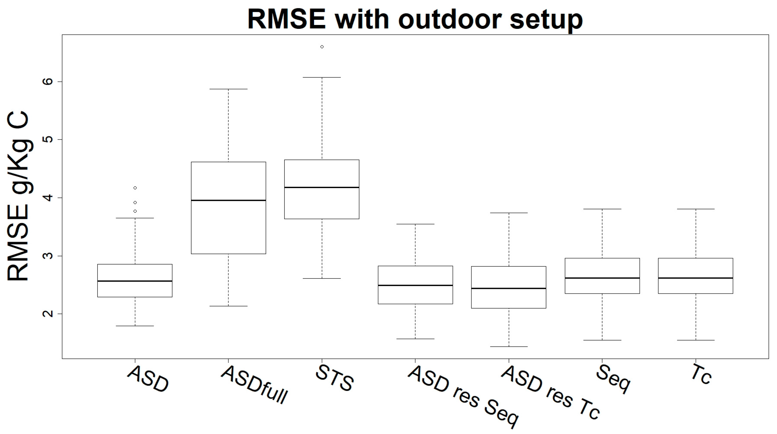
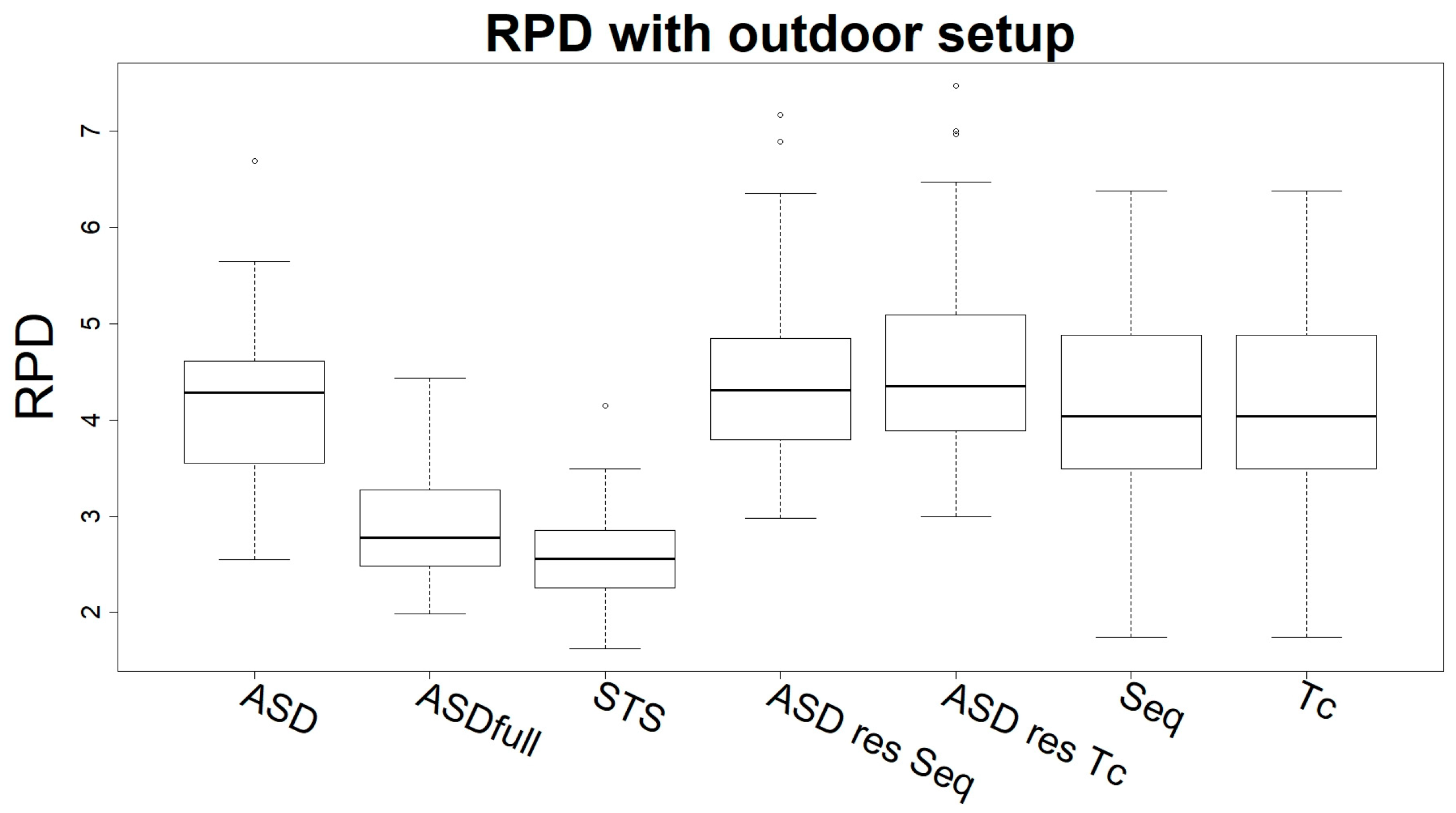
| “ASD” | 3 | 0.51 | 2.2 | 5.3 | 6.2 | 0.96 | 5 | 0.8 | 2.6 | 4.2 | 4.9 | 0.94 |
| “ASDfull” | 3 | 1 | 2.1 | 5.4 | 6.9 | 0.96 | 7 | 2.7 | 3.9 | 2.9 | 3.6 | 0.89 |
| “STS” | 3 | 2.4 | 2.9 | 3.9 | 4.5 | 0.94 | 6 | 3.1 | 4.2 | 2.6 | 3.0 | 0.85 |
| “ASD res Seq” | 4 | 0.48 | 2.4 | 4.7 | 5.1 | 0.95 | 4 | 0.45 | 2.5 | 4.4 | 5.6 | 0.95 |
| “ASD res Tc” | 5 | 0.17 | 2.6 | 4.4 | 5.3 | 0.95 | 5 | 0.79 | 2.5 | 4.5 | 5.2 | 0.95 |
| “Sequoia” | / | / | / | / | / | / | 4 | 0.82 | 2.7 | 4.2 | 5.1 | 0.94 |
| “Tc” | / | / | / | / | / | / | 5 | 2.2 | 3.3 | 3.5 | 4.5 | 0.93 |
| Dataset | No Spectral Correction | Spectral Correction | |||||||||
|---|---|---|---|---|---|---|---|---|---|---|---|
| Calibration | Validation | RE% | RMSE | RPD | RPIQ | R2 | RE% | RMSE | RPD | RPIQ | R2 |
| Lab “ASDshort” | Out “ASDshort” | −0.4 | 3.4 | 3.2 | 4.0 | 0.9 | 0.6 | 3.4 | 3.2 | 3.8 | 0.9 |
| Lab “ASD” | Out “ASD” | −5.3 | 3.1 | 3.5 | 4.3 | 0.9 | −18.3 | 5.7 | 2.3 | 2.5 | 0.7 |
| Lab “ASDfull” | Out “ASDfull” | −24.4 | 4.6 | 2.5 | 3.0 | 0.8 | 20.9 | 4.7 | 2.4 | 2.6 | 0.8 |
| Lab “STS-VIS” | Out “STS-VIS” | 34.7 | 7.8 | 1.4 | 1.6 | 0.4 | 14.6 | 3.7 | 2.9 | 3.2 | 0.9 |
| Lab “ASDshort” | Out “STS-VIS” | 11.5 | 4.4 | 2.5 | 2.9 | 0.8 | −7.8 | 4.2 | 2.6 | 3.1 | 0.8 |
© 2019 by the authors. Licensee MDPI, Basel, Switzerland. This article is an open access article distributed under the terms and conditions of the Creative Commons Attribution (CC BY) license (http://creativecommons.org/licenses/by/4.0/).
Share and Cite
Crucil, G.; Castaldi, F.; Aldana-Jague, E.; van Wesemael, B.; Macdonald, A.; Van Oost, K. Assessing the Performance of UAS-Compatible Multispectral and Hyperspectral Sensors for Soil Organic Carbon Prediction. Sustainability 2019, 11, 1889. https://0-doi-org.brum.beds.ac.uk/10.3390/su11071889
Crucil G, Castaldi F, Aldana-Jague E, van Wesemael B, Macdonald A, Van Oost K. Assessing the Performance of UAS-Compatible Multispectral and Hyperspectral Sensors for Soil Organic Carbon Prediction. Sustainability. 2019; 11(7):1889. https://0-doi-org.brum.beds.ac.uk/10.3390/su11071889
Chicago/Turabian StyleCrucil, Giacomo, Fabio Castaldi, Emilien Aldana-Jague, Bas van Wesemael, Andy Macdonald, and Kristof Van Oost. 2019. "Assessing the Performance of UAS-Compatible Multispectral and Hyperspectral Sensors for Soil Organic Carbon Prediction" Sustainability 11, no. 7: 1889. https://0-doi-org.brum.beds.ac.uk/10.3390/su11071889