Sustainable Financing for Sustainable Development: Agent-Based Modeling of Alternative Financing Models for Clean Energy Investments


Division of Sustainable Development, College of Science and Engineering, Hamad bin Khalifa University, Doha 34110, Qatar
*
Author to whom correspondence should be addressed.
Sustainability 2019, 11(7), 1967; https://0-doi-org.brum.beds.ac.uk/10.3390/su11071967
Submission received: 25 February 2019
/
Revised: 25 March 2019
/
Accepted: 27 March 2019
/
Published: 2 April 2019
(This article belongs to the Special Issue A New Look at Economic Approaches to Environmental, Natural Resources and Energy Economics)
Abstract
:Renewable energy investments require a substantial amount of capital to provide affordable and accessible energy for everyone in the world, and finding the required capital is one of the greatest challenges faced by governments and private entities. In a macroeconomic perspective, national budget deficits and inadequate policy designs hinder public and private investments in renewable projects. These problems lead governments to borrow a considerable amount of money for sustainable development, although such excessive debt-based financing pushes them to unsustainable economic development. This substantial amount of borrowing makes a negative contribution to the high global debt concentration, putting countries’ economic and social development at risk. In line with this, excessive debt-based financing causes an increase in wealth inequality, and when wealth inequality reaches a dramatic level, wars and many other social problems are triggered to correct the course of wealth inequality. In this regard, the motivation behind the study is to develop a set of policy guidelines for sustainable financing models as a solution for these intertwined problems, which are: (1) a financial gap in energy investments; (2) an excessive global debt concentration; and (3) a dramatic increase in wealth inequality. To this end, this study presents a quantitative and comparative proof of concept analysis of alternative financing models in a solar farm investment simulation to investigate the change in wealth inequality and social welfare by reducing debt-based financing and increasing public participation. There are many studies in the literature investigating the evolution of wealth inequality throughout history. However, there is a gap in the literature, and investigating the effects of various policy rules on the evolution of wealth inequality in a future time frame needs to be explored in order to discuss possible policy implications beforehand. In this respect, this paper contributes to the literature by developing simulation models for conventional and alternative financing systems. This enables investigating the changes in wealth inequality and social welfare as a result of various policy implications throughout the simulation time.
1. Introduction
Energy investments have a significant influence on economic growth and development, as widely discussed in the literature [1,2]. Global energy investment accounted USD 1.8 trillion in 2017, and the power sector took the largest portion, which was about USD 750 billion [3]. Electricity investment in the power sector has shifted towards renewables, networks, and efficiency. In line with this, renewable power was valued at USD 300 billion in 2017, accounted for two-thirds of power generation investments, and hit record levels of spending on solar photovoltaics (PVs) [3]. Despite such a considerable amount of current investments, renewables require an annual increase of at least 150% from the current trend between 2015 and 2050, although the rapid advancements in technology reduce significantly the cost of harnessing clean energy [4]. These investments have crucial importance in truly providing affordable and accessible clean energy globally in order to achieve the Paris Agreement target, which is a promise to hold global temperature rise below 2 °C by 2050 [5].
Renewable energy investment plays a critical role in building a sustainable future and a better planet for everyone. Renewables mitigate greenhouse gas (GHG) emissions and provide alternative resources, rather than fossil fuels, for harnessing energy, which is a necessity for economic and social development. However, there was a substantial gap of nearly USD 1.7 trillion in 2017 for financing energy infrastructure, including renewables [3,4]. This statistic shows that finding the required capital is one of the greatest challenges for clean energy investment faced by governments and private entities. In a macroeconomic perspective, national budget deficits and inadequate policy designs hinder public and private investments in renewable projects. These problems lead governments to borrow a considerable amount of money for sustainable development, although such excessive debt-based financing pushes them to unsustainable debt zones [6] and into unsustainable economic development. In a business-as-usual case, renewable energy projects were funded about 90% by debt-based financing from 2009 to 2017 [7]. This substantial amount of borrowing negatively contributes to a high global debt concentration, putting countries’ economic and social developments at risk. In line with this, excessive debt-based financing causes an increase in wealth and income inequality. Piketty advocates that when wealth inequality reaches a dramatic level, wars and many other social problems are triggered to correct the course of wealth inequality [8,9].
The motivation behind this study is to develop a set of policy guidelines for alternative and sustainable financing models as a solution for these intertwined problems, which are: (1) a financial gap in energy investments; (2) an excessive global debt concentration; and (3) a dramatic increase in wealth inequality resulting economic and social crises. In other words, this paper is motivated by finding a solution for the triangle of unsustainability illustrated in Figure 1. In this regard, the objective of the study is to develop policy framework in the financial system to substantially decrease wealth inequality without decreasing total wealth by reducing the debt burden on society and including public participation through private investments. In line with the objective, this study attempts to provide evidence for the following questions. First, if renewable projects are financed excessively by debt-based financing, either from domestic or external creditors, how might it affect long-term sustainable economic and social development for the benefit of the public? Second, the critical question to be answered eventually is: What kind of policy applications for sustainable financing should be developed for renewables, and other public infrastructures, without damaging long-term sustainable economic and social development? In this regard, this study provides a quantitative and comparative proof of concept analysis on alternative and sustainable financings for solar farm investments to investigate their long-term impact on the change in wealth inequality, total wealth accumulation in the economy, and social welfare. To this end, an equity and foundation (not-for-profit)-based financial intermediary (EBIN) is designed in an agent-based model with simple, yet powerful, policy rules and regulations. Also, a banking system is developed to compare the proposed models with conventional financing. The proposed policy framework, which is open to further improvements, encompasses four main components as follows. First, the proposed policy prioritizes individuals in society over large enterprises to participate in solar farm investments as much as their savings. Second, to prioritize individuals, the study limits the investment share in power plants for each shareholder (except for individuals), which are divided into individuals, large enterprises, banks, and equity-based financial intermediaries. Next, the EBIN is designed to become self-sufficient along with the individuals in society after a certain time. Last, the proposed model requires a foundation share from the profit of the EBIN, and thereby this increases the social welfare and equity by spending the money accumulated in the foundation pool for the benefits of the public.
There are many studies in the literature investigating the evolution of wealth inequality throughout the history. However, there is a gap in the literature in investigating the effects of various policy rules on the evolution of wealth inequality in a future time frame. The focus should be to discuss the possible policy implications beforehand. In this respect, the most important contribution of this study to the literature is its development of simulation models for conventional and alternative financing systems that enable an evaluation of the changes in wealth inequality and social welfare as a result of various policy implications throughout the simulation time. In line with this, this study implements the proposed policy regulations resulting in a dramatic decrease in wealth inequality (Gini index) throughout the simulation time. The resulting value is less than the lowest Gini coefficient among 174 countries reported in the Global Wealth Databook, 2018 [10].
2. Literature Review
2.1. Sustainable Development and Global Debt Concentration
The global economy requires radical transformation and thinking to prevent over-consumption, over-production, climate change, air pollution, water waste, desertification, deforestation, land degradation, and biodiversity loss. To this end, the United Nations (UN) envisions a global economic growth in harmony with nature for both individual and national prosperity towards sustainable development goals (SDGs) [11,12]. In this context, economic transformation requires innovating inclusive and productive financing policies and ensuring that such new and alternative financing models promote green and clean consumption and production behaviors within individuals, firms, organizations, societies, and governments [13,14,15,16,17]. However, a high global debt concentration retards this inclusive and productive financing and has a significant, negative impact on sustainable development [6,18]. The global debt-to-GDP (gross domestic product) ratio rose dramatically from 269% in 2007 to 325% in 2016 [19,20]. This increase has an adverse effect on economic growth and financial stability because severe economic and financial crises are expected to happen when the debt ratios exceed a certain limit [21]. Therefore, Ari and Koc recommended innovating equity-based financing models, rather than pure debt-based financing, to maintain debt sustainability [6]. However, this study investigates sustainable financing models by not only reducing the debt burden on society, but also by preventing social stress and redistributing the wealth more equitably.
2.2. Wealth Inequality and Social Inequity
Wealth inequality has influenced significantly, much more than the income inequality, in governing the countries throughout the history as Wilford Isbell King wrote in his book “Whoever controls the property of a nation becomes thereby the virtual ruler thereof” [22]. Wealth distribution, in contrast to income, is best employed as an indicator of possessing economic power in society rather than as a measure of the living standards enjoyed by the public [23]. Therefore, the intimidating power of wealth leads many policy-makers to advocate redistribution of resources by the state through progressive income taxation, which is a good way to increase the material well-being of a society. However, progressive income taxation does not redistribute the economic power, which enables ruling the countries, from a few people to the society. For instance, the Nordic countries (Finland, Norway, and Sweden) have low records of income inequality in the world [24], whereas they have significantly high levels of wealth inequality in the world [10] (see Table 1). There are many studies in the literature investigating the evolution of wealth inequality throughout history and economic models, which have been able to explain this inequality so far [23,25,26,27,28]. However, there is a gap in the literature on investigating the effects of various policy rules on the evolution of wealth inequality in a future time frame by computer simulation. This research targets to reach the lowest wealth inequality among 174 countries, which was reported at 0.498 [10].
Piketty advocates throughout his book, Capital in the Twenty-First Century, that wars, or social unrests, happen to correct the course of history when wealth inequality reaches a significantly high level [9]. Then, the critical question is: What is the global status of wealth inequality? The Global Wealth Databook, 2018 reported the regional Gini indexes of wealth inequality at dramatically high levels, such as 89.7, 90.1, 71.4, 83.6, 85.4, 81.9, 84.3, and 90.4, respectively, in Africa, Asia-Pacific, China, Europe, India, Latin America, North America, and the world [10]. Therefore, policy-makers need to innovate and implement different redistribution mechanisms to reduce wealth inequality to acceptable levels. This study focuses on shedding light and recommending such new policies developed around alternative financing models to decrease the wealth inequality to low levels.
2.3. Financial Localization
Many studies presented and discussed the financial localization and not-for-profit community banking for a healthier economy [29,30,31,32]. Werner advocates that monetary reform should be implemented realistically by establishing many small, local, not-for-profit community banks, such as in the success story of the German economy over the past 170 years [31]. This is because there is an inverse relationship between bank size and the tendency of banks to lend to micro, small and medium enterprises (SMEs), thereby this propensity limits the growth of SMEs [33]. In other words, large enterprises and banks grow together at a significant rate without individuals and SMEs. This leads to capital concentration and centralization in a few hands, which causes social problems as mentioned in the previous subsection. In line with this, SMEs in the UK experience shortage of funding because of a highly concentrated banking system in which five banks account for more than 90% of deposits [29]. On the other hand, Germany has more than 1700 locally headquartered, small savings, and cooperative banks that account for around 70% of deposits [29]. Thus, this might be one of the reasons that Germany has a strong, distributed, and healthy SME network by providing entrepreneur-oriented business with the local banks [34]. Besides, Germany is the only developed country to maintain sustainable public debt levels in comparison to its GDP, as presented in a previous study [6]. In short, financial localization plays a crucial role in providing timely, proper, and adequate amounts of credits for all economic sectors and players, thereby balancing wealth inequality. However, there is a gap in the literature for planning when many small, local, and not-for-profit financial intermediaries should be established. In this regard, this study investigates potential timelines to create a bank or another type of financial intermediary.
2.4. Agent-Based Modeling
Agent-based modeling (ABM) is a powerful scientific toolset for solving complex, real-world problems in many research fields, including economic [35,36,37] and social design [38,39]. ABM adopts a bottom-up approach by designing heterogeneous agents (i.e., people, sector, market, financial intermediaries, and so on) with low abstraction, more details, and micro-level interactions. This study employs a subfield of ABM called agent-based computational economics (ACE), which is motivated by the economic and financial systems [35,40]. In economy and finance, ACE not only brings solutions to complex systems through heterogeneity and adaptivity, beyond equilibrium and rational behavior, but it also gives an opportunity to examine difficult questions about human and environmental interactions, such as agency problems, asymmetric information, collective learning, and imperfect competition [37]. Therefore, ACE is not limited to uniform/symmetric identities or other constraints arising from analytical models.
Furthermore, ACE facilitates the aggregation of values over heterogenous agents (i.e., individuals, power plants, sectors, banks, and so on), while their composition changes dynamically, which is a challenging task [41,42]. This dynamic interdependency of economic agents regarding their behaviors and actions constitutes microeconomics, and the collective behaviors and actions of the agents form a macroeconomic system. In this study, we considerably exploited the aggregation property of ACE in the deterministic model of financing clean energy by incorporating not only funding and carbon intensity, but also incorporating income inequality.
ACE is a relatively new research paradigm; therefore, a limited number of academic papers exist in the vertical dimension on a specific field in the economy, although there are many horizontal perspectives diversified in economics and finance with a growing number of researchers. In energy economics and finance, which is the focus of this study, ACE is largely employed in electricity market regulations [43,44] and energy efficiency models [45,46] (see the paper of Weidlich and Veit for critical literature review on ACE-based electricity sector [47]). However, there are gaps in the literature on modeling and evaluating wealth inequality that look at funding recurring projects in different segments of the population using different financial instruments. In this regard, this study addresses this gap by designing agent-based modeling in investigating the wealth inequality in a society, consisting of large enterprises and individuals, through funding solar farms with various agent types.
3. Methodology
3.1. Platform and Framework Description
The ACE model was implemented in AnyLogic version 8.3. (The AnyLogic Company, Chicago, IL, USA), which is broadly employed in multimethod simulation modeling, namely agent-based modeling, system dynamics, and discrete event modeling. In a technical sense, AnyLogic can be run in any operating system supporting Java Virtual Machine (Oracle Corporation, Redwood City, CA, USA), such as Linux, Windows, and MacOS. Furthermore, AnyLogic enables a custom Java code to be embedded in an agent-based model. Therefore, it provides a substantially flexible modeling and simulation environment without compromising the robustness and scalability level of the model [48]. Also, AnyLogic has a user-friendly graphical user interface for visual model development, although development efforts are relatively moderate [48].
Figure 2 shows the agent-based model and agent interactions that represent the communication of agents with each other. The individual (IN) and large enterprises (LE) agents can be considered as depositors, investors, or both at the same time. The IN and LE behaved as investors when communicating with the equity-based financial intermediary (EBIN). On the other hand, the IN and LE acted as depositors when interacting with the Bank. The EBIN communicated with the special purpose vehicle (SPV) of a power plant (PP) agent through the equity-based financial instrument (EBIS) agent if the equity share was greater than zero (see Figure 3b). The Bank interacted with the SPV of a PP agent through the Loan agent if the loan share was greater than zero (see Figure 3a). The EBIN agent communicated with the foundation pool (FP) if the foundation share was greater than zero. The FP reached out to the public by spending money in public infrastructure, philanthropic purposes, and social venture capital. The FP also enabled the proposed model to provide social impact finance.
This study structured the business model of solar farms with project finance because it was a risk-free business model for the project owner and developer, but not for the investors. However, several essential incentives existed for investors that included power purchasing agreement (PPA), land concession, and tax exemption. The PPA is an agreement between the government and the project developer stating that the government purchases all the electricity produced by power plants. With this regard, project finance brings risk-free financing to investors by applying PPA in solar farms. Project finance puts future cash flows, along with the project’s assets, up as collateral, but not the owner’s or developer’s assets so they are protected them from potential failures. This study focused on the investor side of project financing (see Figure 3c) by investigating debt-based and equity-based financing as the funds for the required amount of money (see Figure 3a,b).
The study proposed policy regulations on alternative financing models for a solar farm with a power purchasing agreement to investigate the change in wealth inequality and social welfare. These policy rules were as follows (see Figure 3b,c):
- The individuals were prioritized to invest in a power plant as much as their savings.
- There were four types of shareholders that included individuals (IN), large enterprises (LE), a Bank, and an equity-based financial intermediary (EBIN). The shareholders were listed in a given order to participate in a power plant investment depending on their savings. For example, assume that the potential shareholders were listed, in order, as individuals and large enterprises. If the individuals did not have enough money for the entire investment, the remaining amount was provided by the large enterprises.
- The shareholders had an upper bound to join in the investment. This upper bound was usually one hundred percent for individuals. In other words, the individuals could invest up to 100% of the total investment of a power plant.
- The equity-based financial intermediary (EBIN) was designed to be a self-sufficient financial intermediary up to a certain limit according to the upper bound.
There was a share for foundation (i.e., not-for-profit institution) out of the EBIN’s profit (see Figure 3c). The foundation share was accumulated in the foundation pool to support future public infrastructure investments. In this regard, the proposed scheme with the inclusion of a foundation could contribute to social welfare.
3.2. Agent-Based Model
This study provided an agent-based model (ABM) on alternative financing models for a solar farm to investigate the change in wealth inequality and social welfare. Figure 4 shows the main constants, variables, and functions in the agent-based model for financing power plants. The class constants represented the same value for all instances of a class during the course of the simulation, while instance constants stored the same value for an object instance, not for all instances, during the lifetime of that instance. Agent-based models require variables and functions to evolve through behaviors and actions. The pointer in Figure 4 was an alias of a variable that accessed a common stack in the memory. In the following subsections, the agent-based model was described for financing the solar farm.
3.2.1. Power Plant (PP) Agent-Type
Power plants play a critical role in generating revenue by producing electricity. This plant required upfront financing for the initial capital expenditure, which was the overnight capital cost (OCC), to become operational. Before generating electricity, there was a construction period (CP) to build a power plant. Producing energy (electricity) was subjected to the operational cost during the lifetime. This study assumed that the PP generated electricity for the period of a lifetime (LT). In addition to net energy output, operational cost, and revenue, PP calculated the carbon intensity of the production and the mitigation levels of carbon emissions. To this end, PP stored the carbon intensity constants for the energy plants powered by natural gas and solar to evaluate carbon emission and mitigation level over the lifetime; this part is explained in the model implementation section.
The special purpose vehicle (SPV), inside the PP, played a central role in managing the financial activities of the power plant by borrowing and fundraising for the capital expenditures, paying back loan installments, expensing for the operational cost, and distributing the net profit to the shareholders. Therefore, the SPV had the fundamental responsibility of communicating with external agent-types through message-passing algorithms. It communicated with the Bank (conventional financial intermediary) agent-type through the loan agent-type and an equity-based financial intermediary through an equity-based instrument agent-type.
3.2.2. Depositor/Investor (DI) Agent-Type
The depositor/investor (DI) played a crucial role in providing capital resources. This study designed two agent populations from DI agent-types, namely individuals and large enterprises. We assumed that the individuals (INs) consisted of 100,000 agent populations of people, micro, and small enterprises, which were governed and owned independently by the citizens. The large enterprises (LEs) comprised a ten-agent population from large corporate and private entities. These agents from IN and LE populations could deposit their savings into the bank agent or invest through the equity-based financial intermediary (EBI) agent. They could perform both actions at the same time or keep their money in their safe. Therefore, LE and IN had three time-dependent variables in which they could save their money, namely, bank pool (BP), EBI pool (EBIP), and safe pool (SP) for the related agent. The bank pool represented the savings deposited in the bank, the EBI pool stored the capital resources in the EBI for future investments, and the safe pool kept the money as “mattress money”. For the sake of simplicity, we assumed that these saving pools (i.e., Bank, EBI, and safe) in each population (IN and LE populations, separately) had a uniform distribution in each time step. For example, if the total bank pool of IN population stored $100,000, then each has $1 in their bank pool because of the uniform distribution and population of 100,000. As proof of concept, this assumption enabled the calculation of wealth inequality by Gini index over the simulation time.
3.2.3. Loan Agent-Type
The loan agent-type played a profound role in financing the power plants. While creating a PP agent, in the initial stage, PP communicated with the Bank agent to be financed by a loan agent. This stage was called an agreement between the bank and power plant in order to create loan agent with a loan amount (LA), loan interest rate (LIR), and loan period (LP). The LA denoted the loan demand defined by the loan share (LS) of the overnight capital cost (OCC), as in the equation LA = OCC × LS. The OCC was a constant value of the PP, and LS represented the environmental constant. There are several functions explained in Appendix A such as set lending, calculation installment, and future values.
3.2.4. Bank Agent-Type
The bank had a significant role in evaluating a conventional financial system. This study assumed that the bank agent is a simple financial intermediary according to the theories of banking structure. The financial intermediation theory (FIT) considers a bank just as a non-bank financial institution, the only difference is the main activity of banking, which is a depositing and lending business. Therefore, the banks in the FIT differ from the banks in the fractional reserve theory and the credit creation theory by having no power to create money out of nothing [31].
This study assumed that there was only one bank in the simulation environment. This assumption was based on financial localization and no competition between banks. In detail, we considered a closed economic system where capital resources were limited to geographical location. Therefore, there was not enough resources and need to establish a second bank. In this regard, there was no competition because the banking system formed a monopoly. However, we assumed that this bank could communicate with the agents out of the environment. In this way, it could utilize the idle cash in money pools, which was called the bank liquidity (BL), by lending to the interbank lending market outside of the environment. It is worth to note that the large enterprises and individuals cannot reach out to the environment, such as to another bank or another agent, to deposit or lend their savings.
The bank operated with three stock variables, namely, large enterprise money pool (LEP), individual money pool (INP), and the bank profit pool (BPP). The LEP and INP not only stored the savings of large enterprises and individuals but also deposited the interest issued by the bank for the savings. The central bank required the reserve deposit from the bank that was the share of the bank liability. In return, the central bank payed interest on the reserve by the interest of the required reserve. The BPP represented the interest earnings from the central bank and the interbank lending market (which provided interest to the bank in return for lending idle bank liquidity). Furthermore, these money pools (LEP, INP, and BPP) could be reduced by withdrawals for investment, and they could be increased by profit deposits from the power plant. These actions were conducted by several functions, as explained in Appendix B.
3.2.5. Equity-Based Financial Instrument (EBIS) Agent-Type
The EBIS agent played a central role in developing alternative financing models for the building of a power plant. Initially, a new PP agent interacted with the equity-based financial intermediary (EBIN), explained in Section 3.2.1, to make an agreement for the fundraising of capital expenditures. If the EBIN had liquidity, or was able to fundraise from the LE and IN agents to invest in a new power plant, then they agreed with the message-passing algorithm. In this case, the EBIN created the EBIS agent for the investment of a new power plant. The investment represented the equity amount (EA), EA = OCC × ES, where the OCC denoted the overnight capital cost of the power plant. The ES was a constant value in the environment.
The investment policy, defined in the environment, formed the shareholder structure of a power plant. This structure included the ordered list of the shareholders and the corresponding upper bounds of each one of the participants. The ordered list was a prioritized collection of the IN, LE, EBIN, and the BANK agents. The upper bound (UPIN, LE, EBIN, Bank) indicated that each agent in the ordered list could participate in the power plant project to their certain corresponding limit, even if this agent had more liquidity than the upper bound. The EBIS agents calculated the fundraising amount and the holding ratios under the investment policy. To this end, this agent-type contained the following functions, namely, set investments and set shares. These are explained in Appendix C.
3.2.6. Equity-Based-Intermediary (EBIN) Agent-Type
The EBIN agent-type played a profound role in delivering policy implications for more sustainable financing. Equity-based financing balanced the debt-based financing by sharing risk with the project developer instead of transferring the entire risk to the project developer, as in conventional banking. In return, equity-based financing offered more profit than the deposit interest in the debt-based financing because it carried more risk. However, this study eliminated the potential risks by the government guarantee. In the initial stage of the project, the government signed a power purchasing agreement (PPA) with the project developer, thereby, the risk was removed from the project developer and was transferred to the government. Therefore, the future cash flows of a power plant substituted for the potential risk of the investment. In other words, the PPA served as collateral for the project. Furthermore, there was a foundation pool if the EBIN was a non-profit financial intermediary. The foundation pool was an account to deposit the excess money of the EBIN according to the investment policy. The excess money was a surplus amount that was more than the authorized investment of the EBIN. In other words, the investment policy authorized the EBIN to invest in a power plant up to a certain limit. Beyond this limit, the excess money was transferred to the foundation pool. Depending on the policy, this model enabled to utilize the foundation pool for the benefit of the public, such as for social venture capital and public infrastructure (i.e., education and health facilities, bridges, railways, highways, and so on).
The conventional banks, first, evaluate the investor’s financial risk status by analyzing the past credit score from the credit bureau. The individuals, micro, and small enterprises showed a lack of creditworthiness because they usually did not have any credit score at all, or they have poor risk scores because of the liquidity and agency problems of the SME. Therefore, the credit score led the banks to lend mostly to the large enterprises because they have low financial risk and high creditworthiness scores. In this case, the individuals, micro, and small enterprises encountered the capital resource scarcity. This fact was a problem, which led to economic inequality in the short run and social inequity in the long run. As a result, this system made the rich richer, and the poor poorer. The ultimate consequence of economic and social inequity might be social unrest, violence, political chaos, and even war [9].
There are several functions to perform actions and operations of the EBIN that are explained in Appendix D.
3.2.7. Government Agent-type
The government played a vital role in balancing social and economic inequity. The government agent-type provided incentives for building a power plant by prioritizing the individuals, micro, and small enterprises. This prioritization was the backbone of the model’s investment policy. The government was responsible for regulating the policy by employing the environment variables.
There existed several essential incentives, along with the prioritization of the IN agent-type, which were power purchasing agreement (PPA), land concession, and tax exemption. The PPA was an agreement between the government and the project developer stating that the government purchased all the electricity produced by power plants. The EBIN recognized the PPA as risk protection from the electricity market turmoil, and the Bank considered the agreement as collateral. It is important to note that this study assumed that the government incentivized equity-based financing by compensating price discrepancy in favor of equity-based funding. Under this assumption, the government always sold electricity at a fixed price, although the levelized cost of electricity changed for the government by different shares of loan and equity. In addition, this study focused on wealth distribution under different policy settings without any intervention on income and wealth by the government; therefore, income and wealth taxations were out of scope.
A land concession was a place granted for building a power plant. The tax exemption was tax relief for the investors subjected to selling electricity generated by the power plants. In return, the government could receive environmental, economic, and social benefits as a result of this policy implementation and incentivization. First, this model, which was implemented in renewable energy plants, brought environmental benefits by reducing CO2 emissions. Next, economic benefits fulfilled more equitable income through society, reduced debt dependency on energy security, and provided more individual participation. Last, this financing model delivered more social equity by exploiting the foundation pool to invest in human capital development, public infrastructure, and social venture capital.
3.2.8. Environment
The environment (ENV) was a top-level agent that contained all agents explained above in the simulation. The variables and constants of the ENV were defined below. Further explanations about all other variables of the environment are listed in Appendix E.
Equity share (ES). Equity share indicated the investment share of capital expenditure in a power plant. The EBIN agent calculated the total investment amount by the equity share. In other words, the equity amount (henceforth interchangeable with investment amount) was EA = OCC × ES, where OCC represented the overnight capital cost.
Loan share (LS). Loan share represented the debt percentage of the overnight capital cost that was borrowed from the Bank by the SPV of a power plant. The SPV computed the loan amount (LA) by . It is worth to mention that the sum of equity and loan share was equal to 1, ES + LS = 1.
Project developer (DEV). This model assigned one of the agents (IN, LE, EBIN, and Bank) to the DEV object-variable. The project developer might take profit shares in exchange for the responsibilities of building and managing a power plant.
Project developer share (DEVS). The project developer can participate in profit distribution as a shareholder without capital investment because the DEV was responsible for building and managing the project. The DEVS represented the project developer’s profit share, which was a preference share. Preference shares were shares of a power plant with dividends that were paid out to the preferred shareholder (i.e., DEV) before common stock dividends for other agents were issued.
Equity intermediation share (EIS). In return for only raising funds, the EBIN had preference shares in profit distribution, which was the operating profit of the intermediary. This profit was allocated by the equity intermediation share, which corresponded to profit for the EBIN and funding cost for the shareholders. The EBIN could also receive profit apart from the intermediary share by investing in a power plant with the money it owned.
Foundation share (FS). This constant represented the foundation share of the EBIN’s gross profit. The EBIN transferred the foundation amount to the foundation pool, which was calculated by multiplying the gross profit by the foundation share.
Shareholder list (SL). The shareholder list played an important role in prioritizing the shareholders by assigning the agents (IN, LE, EBIN, and Bank) in an ordered list. The EBIN decided the investment shares in order according to the shareholder list, which corresponded to the prioritization of the agents under the investment policy. For example, under the assumption of SL = {O(IN,EBIN,LE,Bank)}, the EBIN raised the investment fund by collecting, in order, the money from the IN, EBIN, LE, and Bank.
Shareholder upper bound (SUPa). This upper bound indicated that the shareholders could invest in a power plant up to a certain limit as a share of the overnight capital cost. In other words, the EBIN collected money from the first agent in the shareholder list up to the first agent’s SUPa of the overnight capital cost. If the collected amount reached the limit, then the EBIN sought the remaining amount in the second agent of the shareholder list, and this procedure continued up to the last agent in the list.
Carbon intensity (CIpp). The CIpp denoted the life cycle emissions of carbon intensity for an energy plant powered by natural gas (NG) and a solar farm (SF), separately, where represented the set of power plants.
Functions of the Environment
The calculation of the Gini index and illiquid assets were the main functions needed to evaluate the wealth accumulation and inequality, which are explained as follows.
Calculate illiquidity. The illiquidity assets played a key role in computing the wealth and, thereby, comparing the proposed policies with conventional financing policies. The illiquidity was equivalent to the total present value of the future profits of the remaining years from the lifetime of powerplants. However, we assumed that the illiquid assets of the shareholders for each year in the construction period were assigned to a value that was the present value of the first year of operation divided by the construction years as given in Equation (1).
where represented the present value of the future profit of the power plant for year , and denoted the construction period in years. In the meantime, employed the inflation rate as a discount rate for year . The illiquidity was distributed into the agents as in Equation (2).
where represented the investment share of agent . Henceforth, we could calculate the total illiquid assets of an agent (i.e., IN, LE, EBIN, and Bank) at time t as shown in Equation (3).
where represented the total illiquid assets of an agent at time .
Calculate Gini index. The Gini index played a primary role in evaluating new policies and comparing the proposed financing models with conventional financing models in terms of wealth inequality. This study computed the gini by taking half of the relative mean of absolute difference. The mean absolute difference represented the average absolute difference of all pairwise wealth comparisons of the entire population, and then the relative mean absolute difference was calculated as the mean absolute difference divided by the average. In this regard, the gini is shown in Equation (4).
where was the wealth of entity (IN, LE, Bank or EBIN), and there were entities. This study can simplify the summation in Equation (4) because of the assumption of uniform distribution of liquidity (and thereby illiquid assets) within the populations (individuals and large enterprises). First, this uniformity enabled us to calculate each entity’s wealth in each group (individuals, large enterprises, bank, and EBIN), which is shown in Equations (5)–(8).
where and represented the average wealth for a person and a large enterprise as money pools (and illiquid assets accordingly), and were distributed uniformly according to the assumptions. As a reminder, this model consisted of two financial intermediaries, namely the bank and the EBIN; therfore, their average wealth, and , were equal to their total assets. TAIN and TALE corresponded the total assets, sum of liquid and illiquid assets, for individuals and large enterprises. Next, we calculated the pairwise absolute differences of each entity’s wealth, as given in Equations (9)–(14).
Afterwards, we simplified Equation (4), which is shown in Equation (17) following Equation (15) and (16).
This study also investigated the scenarios based on non-profit EBIN agents, which transferred all the excess money to the individuals through the foundation. In this case, the EBIN’s wealth ( was employed only for the benefit of the public. We thereby extracted from the related equations, and the foundation assets were added into individual’s wealth as in Equation (18). This change affected the pairwise absolute differences and accordingly, as shown in Equation (19) and (20).
Then, the Gini index transformed into Equation (23) by following Equation (21) and (22).
3.3. Model Implementation: A Solar Farm
Qatar has made limited progress in renewable energy generation despite the great potential for harnessing solar power. Therefore, the current share of renewable energy over the total generation capacity, which is planned to reach 13 gigawatts (GW) by 2019 [49], is negligible [50]. However, the government set quite promising targets to achieve a considerable share in total power capacity and to diversify the energy mix. The targets for renewable power in the first and second stage are 2% and 20% of total energy production by 2020 and 2030, respectively [51]. In line with this, the Ministry of Energy and Industry is developing and implementing a strategy for utilizing renewable energy along with its policy [50]. In addition, a group of researchers from Kahramaa, which is Qatar general electricity and water corporation, has developed a solar farm project along with its feasibility and geographic location, with the collaboration of Hamad Bin Khalifa University (HBKU) as a capstone project [52]. In this study, we adopted their project’s input data and assumptions for the technical part of the power plant agent (see the power plant part of Table 2). Also, Table 2 summarizes all the inputs and assumptions in this study. It is important to note that the project developer and the government signed a power purchasing agreement, which was a legal contract stipulating that the government buys all electricity generated by the power plant during its lifetime.
Policy Scenarios
The simulations ran under predefined inputs and assumptions (Table 2) and policy variables (Table 3). These policy variables were explained in Section 3.2.8. They had a significant influence on the simulation results because they affected the wealth accumulation in size (how much wealth will be accumulated) and place (in which agent it will be accumulated). However, this study set these policy variables as constant because our goal was to evaluate how the changes in the parameters of the project developer, loan share, equity share, project shares (or shareholder limits), non-profit EBIN, and foundation share will affect the wealth accumulation and Gini index.
In this study, seven financing scenarios were evaluated on the solar farm project in Qatar, which were divided into two groups. First, we performed three of the scenarios for comparison against the proposed policies. Second, this study conducted the remaining four scenarios by adding a new policy on top of the previous simulations in each step. The comparative analysis and the performance of the policies will be discussed in Section 4. The policy scenarios are summarized in Table 4. The details of each policy scenario are given in the following explanations.
Scenario 1: The policy of Scenario 1 was based on pure loan-based financing of a power plant, which meant that the debt-to-capital ratio was one hundred percent. This scenario was designed for comparison purposes against the proposed models and a part of the sensitivity analysis of the equity and loan share parameters. In this scenario, the project developer was a consortium of large enterprises in the model. Since the project fund was one hundred percent debt-based financing, the predefined project-shares were valid for the shareholders. Therefore, this feature enabled us to define large enterprises with one hundred percent shares of the project. In this scenario, there was no need to establish the EBIN because of the pure debt-based financing.
Scenario 2: The policy of Scenario 2 was based on mixed financing (a common practice) of a power plant. This study considered this case as a business-as-usual case for the comparison purposes against the proposed models because the average of the project companies had a debt-to-capital ratio of 70% and an equity-to-capital ratio of 30% [55]. In this scenario, the project developer was a consortium of large enterprises. Since the project fund was mixed financing, the project-shares could not be predefined as in the pure debt-based financing. This study assumed that the capital investment ratio of the shareholders dynamically determined the project shares in each power plant. In other words, the shareholders would own the power plant at the level of equity shares they invested in the project. This feature depended on agent liquidity and predefined shareholder limits. The shareholder limits indicated that the shareholders could invest in a power plant up to a certain limit as a share of the overnight capital cost, even if they had more liquidity. In this scenario, the shareholder limits were (LE, Bank, IN, EBIN)→(1.0, 1.0, 1.0, 1.0), which meant the LE, Bank, IN, and EBIN could invest in a power plant up to one hundred percent of the overnight capital cost. Last, there was a need to establish the equity-based financial intermediary, the EBIN, to fundraise the required equity amount. This EBIN was a profit-based intermediary, thereby it did not transfer any money to the foundation pool.
Scenario 3: The policy of Scenario 3 was based on pure equity-based financing of a power plant, which meant that the equity-to-capital ratio was one hundred percent. In this case, the project developer was a consortium of large enterprises. The shareholder list and the corresponding shareholder limits were (LE, Bank, IN, EBIN)→(1.0, 1.0, 1.0, 1.0). Since the EBIN was the profit-based financial intermediary, there was no money accumulation in the foundation pool. It is worth to note that this scenario is not a common practice because large enterprises are not usually willing to invest in a project by putting in 100% of the equity. However, this scenario was designed for the comparison purposes against the proposed models and as a part of the sensitivity analysis of the equity and loan share parameters.
Scenario 4: The policy of Scenario 4 was based on pure equity-based financing of a project, which meant that the equity-to-capital ratio was one hundred percent. This part was the same as Scenario 3. However, this study applied a new policy by changing the project developer and reordering the shareholder list. The project developer was altered from the LE to the EBIN. The shareholder list and the corresponding shareholder limits were (EBIN, IN, LE, Bank)→(1.0, 1.0, 1.0, 1.0). This change meant that the project developer sought, in order, the required funds from EBIN, IN, LE, and Bank without any share limits. If the first agent did not have adequate capital to invest in total overnight capital cost, then the project developer took all available funds from the first agent and asked the remaining amount from the next agent in the list. Meanwhile, there was no money transfer from the EBIN to the foundation pool since the EBIN was still a profit-based intermediary.
Scenario 5: The policy of Scenario 5 was based on one hundred percent equity-based financing of a solar farm. The project developer and the shareholder list remained the same as Scenario 4. However, the shareholder limits were changed to (EBIN, IN, LE, Bank)→(0.20, 1.0, 1.0, 1.0). This policy change meant that the project developer raised the funds first from the EBIN up to the 20% of the overnight capital cost, which was a shareholder limit. Even if the EBIN had more liquidity, it could not invest in a power plant more than this limit. Therefore, excessive money, which was earned from the power plants and intermediation shares, would be accumulated in the EBIN’s money pool. There was no money transfer from the EBIN to the foundation pool since the EBIN was still a profit-based intermediary.
Scenario 6: The policy of Scenario 6 was based on full equity-based financing of a solar power plant. The project developer, the shareholder list, and the shareholder limits remained the same as Scenario 5. In this policy, the parameters of not-for-profit EBIN and the foundation share were set to “true” and 50%, respectively. This study applied these conditions in two successive stages. First, the EBIN transferred 50% of its own earnings to the foundation pool up to reaching the shareholder limit, which was 20% of overnight capital cost. Second, beyond this limit, all excessive money was transferred to the foundation pool without considering the foundation share. This study assumed that the foundation pool was distributed equally throughout the society in terms of public infrastructure, health centers, education facilities, and so on.
Scenario 7: The policy of Scenario 7 was based on full equity-based financing of a solar power plant. The only difference from Scenario 6 was that we removed the banking system completely from our simulation model. This scenario was a hypothetical case because there is no such system in which banking is nonexistent. However, this model enabled us to evaluate the behavior of the wealth accumulation and Gini index when banking was absent. Thus, this case provided a few glimpses for developing a future policy to adjust the existing banking system.
4. Results and Discussion
The main results of the seven scenarios in financing solar farms are summarized in Table 5, which were divided into the policies for comparison purposes and the proposed policy implications. These results indicated that the investment policy in Scenario 6 based on the proposed model had the best performance compared with the policies in the other six scenarios. This was because Scenario 6 was the optimum policy set among these scenarios in terms of the simultaneous Gini index minimization (i.e., increased equality among the stakeholders) and the wealth maximization. It is worth noting that Scenario 7 became deficient in terms of total wealth accumulation, although the Gini index was substantially low. In environmental aspects, there was a significant decline in carbon emissions at the same level for each scenario. The mitigation of carbon emissions climbed rapidly from around 0.20 million tons to 2.56 million tons of CO2 equivalents in a year. This level of carbon mitigation can have a positive effect on public health, and it helps to fulfill Qatar’s environmental commitments [50]. This result showed that this study satisfied environmental sustainability requirements.
The total cash accumulations were about QAR 25.5 billion, 26 billion, and 28 billion, respectively, in Scenarios 1, 2, and 3 (see Figure 5). In these scenarios, the project developer was a consortium of all large enterprises. Therefore, the individuals had a steady, but minimal, increase in cash accumulation throughout the simulation time because they earned only interest on their deposits in the bank. In detail, the individuals did not invest in a power plant, as can be seen in the illiquid asset accumulation graph (see Figure 5), because the project developer raised the required funds without demanding any amount from individuals according to the shareholder list and limits. For the bank, the trend of cash accumulation was quite similar, but it reached a peak at different levels in each scenario. The highest levels were around QAR 15 billion, 12 billion, and 5.5 billion in Scenario 1, Scenario 2, and Scenario 3, respectively. As can be understood from this result, the liquidity accumulated in the bank decreased as the equity share increased for the power plants. This was because the project developer withdrew more money from the bank to invest more in the power plants, and the EBIN earned more profit as the financing was more equity-based. It is worth to note that the EBIN did not deposit its profit into the bank. If the debt-to-capital ratio was 100%, as in Scenario 1, then the cash accumulation for the EBIN did not occur over the simulation time.
Large enterprises, on the other hand, showed different behaviors in the cash accumulations of Scenarios 1, 2, and 3 because of their role as the project developer. The liquid assets of the large enterprises reached a peak at different levels in 2069 (end of simulation time) at QAR 9.3 billion, 11.3 billion, and 17.9 billion in Scenarios 1, 2, and 3, respectively. This significant increase was because the consortium of large enterprises invested in the power plants with more equity that rose in each successive scenario. Therefore, the illiquid asset accumulation rose according to the increase in equity in the short-run, thereby increasing the liquid asset accumulation in the long run. In Scenario 1, there was a slight fall in the cash accumulation from 2028 to 2032 following a gentle and steady increase. The reasons for this decrease were twofold. First, the loan installments in debt-based financing of 100% were greater than the profit between the third and tenth year of power plant operation. Second, the loan installments reached a level in 2028 in which the interest earnings from the cash deposited in the bank, and positive net profits could not compensate the deficits from the paybacks. However, the cash accumulation began to recover in 2032 right after closing the loan for the first power plant in Scenario 1. Afterward, the liquid asset for the large enterprises grew rapidly up to the end of the simulation. In Scenarios 2 and 3, the cash accumulations again hit low points in 2031 and 2027, respectively. This was not because of the negative net profit, as in Scenario 1 (net profits were positive in these cases), but because of the withdrawals from the bank for the investment. In other words, this diminishing money was transformed into illiquid assets to generate more liquid assets in the long run. In the meantime, the bank’s liquid assets exceeded the cash accumulations of large enterprises in 2031 and 2062 in Scenarios 1 and 2, respectively. In Scenario 3, the large enterprise’s curve, however, was always higher than the bank’s liquid assets.
It is worth to note that negative profits in Scenario 1 could be solved by prolonging the loan period, but this would cause less illiquid asset accumulation (also wealth accumulation), and it was difficult to compare the results with the other scenarios. Therefore, we set the loan period as constant to eliminate discrepancies in the results. Furthermore, this was one of the reasons that the debt-to-capital ratio of 70% was more common practice in the project market [55], because the net profit would not be negative in this case.
The results showed that the illiquid asset accumulations in Scenarios 1, 2, and 3 reached equilibrium states in 2044, which was equivalent to 25 years from the simulation start. This period was the lifetime of a power plant. Next, the illiquid asset accumulations leveled off and remained constant at different levels until the end of the simulation time. These levels were around QAR 2 billion, 3 billion, and 5.5 billion for large enterprises in Scenarios 1, 2, and 3, respectively. There was also a small share of the EBIN in Scenario 2 (QAR 325 million), and Scenario 3 (QAR 620 million) because of the intermediation share. This finding implied that illiquid asset accumulation increased with the rise of equity-based financing, and vice versa. In return, the cash accumulation also grew in the long run.
The wealth was the sum of the liquid and illiquid assets. The total wealth accumulations were around QAR 27.7 billion, 29.3 billion, and 34.4 billion, respectively, in Scenarios 1, 2, and 3 (see Figure 5). This result indicated that wealth accumulation increased in each scenario as equity share rose, and vice versa. This was because illiquid assets that generated liquid assets depended on equity participation. In Scenarios 1, 2, and 3 the bank and individuals accumulated only cash assets throughout the simulation time, as can be seen on the graphs of the illiquid asset accumulation. Therefore, the wealth accumulations of the bank and individuals were equivalent to their cash accumulations. The bank’s wealth reduced in Scenarios 1, 2, and 3, while total wealth rose in those cases. In Scenario 1, the bank’s wealth exceeded the individual and then the large enterprise’s wealth, whereas it was always at lower points than the large enterprises in Scenarios 2 and 3. This was because, in Scenarios 2 and 3, the potential wealth of the bank was transferred to the large enterprises and the EBIN through the investments in illiquid assets as the shares of equity increased in the power plants. In Scenario 2, the EBIN was always lower than the bank; however, it was higher than the bank’s wealth by 2063 in Scenario 3, and the bank exceeded the EBIN from that time on.
This study measured the Gini index to evaluate the change in economic inequality and compare the proposed policies with Scenarios 1, 2, and 3 (see Figure 5). In these scenarios, there was an upward trend in economic inequality over the simulation time. The change became sharper in these cases when the equity shares gradually increased against the loans. This was because the large enterprises, whose population was only ten, accumulated more cash through more illiquid assets, as they were the project developer. In addition, they earned more interest from the bank as they collected and deposited more profit from the power plants funded by more equity-based financing. These results showed that sole equity-based financing, without any policy application, did not benefit economic and social equity; it even harmed more, as can be seen in Scenario 3. As a result, the rich became richer and the poor stay poor.
This study introduced alternative financial models by adding a new policy rule on top of the previous models in each scenario. This approach formed Scenarios 4, 5, and 6, as follows (see Figure 6). In Scenario 4, which was based on Scenario 3, there were two policy changes in the parameters of project developer and shareholder list. First, the project developer was altered from a consortium of large enterprises to the equity-based intermediary. Second, the model prioritized the EBIN and then individuals in the shareholder list, as in the order of (EBIN, IN, LE, and Bank). In Scenario 5, the study put forward another policy change, in addition to Scenario 4, that limited the EBIN’s investment in the power plants to a maximum of 20%. In Scenario 6, the model incorporated the foundation pool by changing the EBIN from a profit-based intermediation to a non-profit-based one. This new policy was expected to increase the social and economic equity by spending its accumulated money towards future public benefits, such as social venture capital and public infrastructure (i.e., education facilities, health centers, bridges, railways, highways, and so on). Scenario 7, which was based on Scenario 6, was a hypothetical test case assuming that there was no bank in the financial system at all. The other parameters were entirely the same as Scenario 6. This case provided evidence to the discussions about the banking system in the literature by evaluating wealth inequality when there was no bank in the model.
In Scenarios 4, 5, and 6 the EBIN (project developer) raised the required funds for a power plant with 100% equity-based financing. In these scenarios, the total cash accumulations were about QAR 25.9 billion, 25.3 billion, and 25.4 billion, respectively (see Figure 6). There was a little fluctuation in the liquid around the average of QAR 25.5 billion. This value was very close to the liquid asset accumulations in Scenarios 1 and 2. In other words, in the proposed models, the cash accumulations stayed almost at the same level with the accumulations in Scenario 1 and Scenario 2. However, there was a small difference between Scenario 3 and the proposed models by around QAR 2.5 billion. This was because a consortium of the large enterprises was the project developer in Scenario 3, and the power plant was funded by an equity-to-capital ratio of 100%. Therefore, the illiquid assets were accumulated in a few hands (the large enterprises and the bank), which caused a monopoly; that much assets in the large enterprises generated more profit in the long run. In addition, they deposited more money into the bank because there was more profit, and they also earned more interest on their profit from the power plants. This monopoly, as can be seen in the dramatic increase in Gini index of Scenario 3, incurred an unsustainable financing model and an undesired case for the public/common good. None of the proposed models suffered from this much increase in economic inequality.
In Scenarios 4, 5, and 6, the illiquid asset accumulations reached the equilibrium state, which was the state that the illiquid assets of all the shareholders remained constant at a certain level, around 2060 (see Figure 6). This result showed that the proposed models reached the equilibrium state about 16 years later than Scenarios 1, 2, and 3. This was only because the project developer and the order of shareholder list were changed to the EBIN and (EBIN, IN, LE, and Bank), respectively, in the proposed policies. The underlying reason for the delay in reaching the equilibrium state is given as follows. The EBIN did not have adequate liquidity to finance a power plant at the beginning of the simulation. The EBIN raised the required funds by following the order in the shareholder list (this order can be optimized to set the right policies in a more complex and diverse presence of players). Therefore, the individuals were the first in the list right after the EBIN to finance the power plant, but they also did not have enough money to build the successive projects. Thus, the EBIN collected the remaining amount from the large enterprises. In each successive project, the EBIN earned profit not only from the intermediation share (10%) and project developer’s share (15%), but also from the investment in the project, and thereby the EBIN owned more liquidity to invest in the long run. In the meantime, the individuals also earned profit from the power plant after transforming their initial liquidity to the illiquid assets so that they could invest more in future power plants in the long run. It is worth reminding that the proposed policies prioritized the EBIN and individuals for fundraising the power plant. Therefore, the proposed policies utilized the delay of 16 years to make the EBIN, or individuals, or both, self-sufficient for building a power plant according to the shareholder limits.
In Scenario 4, the cash accumulation of the EBIN reached a peak at QAR 6.2 billion in 2069, which was the end of the simulation (see Figure 6). However, this liquidity remained constant at zero until 2034 because the EBIN transformed all its earnings from the previous power plants to the illiquid assets by investing in the following power plants. After 2034, the EBIN became self-sufficient to finance future power plants. Therefore, the liquidity of the individuals, who were second in the shareholder list, increased while their illiquidity decreased because the power plants were entirely funded from 2034 on by the EBIN. In the meantime, the illiquidity of large enterprises, third in the shareholder list, began to decrease in 2028, six years from the individuals’, because the individuals, along with the EBIN, became sufficient to finance the power plants; thus, there was no need to raise any funds from the large enterprises. This result was also reflected in the Gini coefficient. As can be seen in Figure 6, the wealth inequality steeply reduced in the first two years of the simulation because individuals had adequate money to invest in the first power plant, which took two years to construct. Afterward, the individuals and the EBIN did not have any money to invest in the second power plant, and thereby the EBIN raised the required amount from the large enterprises. Then, the Gini index began to rise sharply because wealth again concentrated in a few hands, large enterprises. However, this rise slowed down as the share of individuals in the power plants increased until 2034, and on. Hereafter, the Gini coefficient began to rise again quickly from 0.765 to 0.874 because the wealth increase of the individuals slowed down. Moreover, the EBIN accelerated its wealth accumulation in this period. This was not only because it was the project developer and first in the shareholder list, but also because it was a profit-based financial intermediary. This time, the EBIN caused an increase in the wealth inequality instead of the bank in Scenarios 1, 2, and 3. Although this rise was not as severe as in Scenarios 1, 2, and 3 where it harmed the economy and society.
In Scenario 5, the model proposed a new policy on top of Scenario 4 that limited the investment share of the EBIN in the power plants to 20%. The remaining policy variables were the same as Scenario 4. This limit provided more investment shares than Scenario 4 for the large enterprises in the short run and the individuals in the long run. As can be seen in Figure 6, the EBIN’s liquidity remained constant at zero until 2026, which was a shorter time period compared in Scenario 4. This was because the EBIN could not invest in the power plants more than 20%, so the liquidity began to increase after 2026. Therefore, the illiquid asset accumulation of the EBIN slowed down and then remained constant at QAR 2.4 billion from 2047 to 2069 (the end of the simulation). From 2026 on, the individuals and large enterprises participated more in the construction of power plants. In this scenario, the large enterprises, however, still continued to invest in the power plants from 2028 to 2032, whereas the EBIN was not required to raise any funds from the large enterprises in Scenario 4 during that period. This was because the EBIN could not invest more than 20%, and the individuals were not self-sufficient to invest 80% of a power plant until 2032. Afterward, the illiquidity of the large enterprises slowed down up to 2060 and then remained constant at zero until the end of the simulation. On the other hand, the illiquidity of the individuals reached a peak at QAR 3.7 billion in 2060 and stayed at the same level up to the end of the simulation. These results also reflected the change in wealth inequality (see the Gini index in Figure 6). The trend of the wealth inequality was almost the same as Scenario 4 until 2030, although it deviated significantly afterward. From 2030 on, the Gini coefficient began to decrease from 0.775 to 0.681, which was even less than the initial value of 0.689. This was because the shareholder limit for the EBIN was set to 20%, and the individuals’ liquid and illiquid assets grew faster than Scenario 4. This result resulted in harm to the economy and society, although this inequality was not as severe as in Scenario 4.
In Scenario 6, this study proposed another policy rule on top of Scenario 5 that set the EBIN as a non-profit financial intermediary (i.e., like a foundation-based institution). Thereby, it transferred excessive profit to the foundation pool for the benefits of the public in the long run. Therefore, the EBIN’s liquidity stayed at a low level, and the foundation pool, following a steady increase in the liquidity, reached a peak at QAR 9.5 billion in 2069. This much money was distributed back to the society by public infrastructure and social venture capital. On the other hand, the illiquid asset accumulation of the individuals stayed at the same level in each data point with Scenario 5. However, the EBIN’s illiquidity increased slower than Scenario 5 because transferring 50% of the profit to the foundation pool caused less investment in the power plants up to 2054. Therefore, the illiquidity of the large enterprises rose more rapidly than Scenario 5 up to 2030 because it compensated the remaining capital deficit induced by the EBIN’s lower investment. These results also reflected the changes in wealth inequality (see the Gini index in Figure 6). There was a sharp decrease in the Gini index in the first two years of the simulation because the individuals had enough capital to invest in the first power plant, as in Scenarios 4 and 5. Despite the erratic rise of the wealth inequality from 2021 to 2026, there was a dramatic decrease from 0.689 to 0.483 over the course of the simulation time. The resulting value was less than the lowest Gini coefficient, 0.498, among 174 countries reported in the Global Wealth Databook, 2018 [10]. In the meantime, Qatar’s Gini index in 2018 was reported at 0.615, which was much higher than 0.483 [10]. Scenario 6 was the optimum policy set among all scenarios in terms of simultaneously minimizing the Gini index (i.e., equality maximization) and maximizing the wealth. As proof of concept, this policy reduced social stress by increasing spending towards the benefit of the public through the foundation pool; and it also decreased social and economic inequality by achieving a more equitable wealth distribution.
Scenario 7 was a hypothetical case that assumed the nonexistence of a banking system in the financial market. The policy variables were held exactly the same as in Scenario 6, but the only difference was that the bank agent was canceled in the model. In this scenario, the foundation pool stayed at the same level as in Scenario 6 because there was no change the EBIN’s illiquidity, and the liquidity accordingly. Thus, the EBIN transferred the same amount of money to the foundation (Figure 7). Therefore, Scenario 7 performed at the same level as in Scenario 6 in terms of public benefits. However, there was a dramatic decrease in the economic inequality from 0.689 to 0.311 over the course of the simulation. The Gini index reached the lowest point of Scenario 6 around 2043, and it continued to decline rapidly until it hit a low point at 0.311 in 2069. This value was much lower than the lowest Gini coefficient, 0.498, among 174 countries [10]. This result showed that in this non-banking scenario economic inequality declined more than a financial market with the banking system. In other words, this hypothetical case indicated that the banking system broke the economic equity.
On the other hand, the large enterprises and individuals reached a peak in liquidity at QAR 4.2 billion and QAR 5.5 billion, respectively, in the end of the simulation. These values were less than Scenario 6 when we compared them with QAR 5.7 billion and QAR 6.2 billion, respectively. This was because the large enterprises and individuals could not deposit their initial capital and profit gains into the bank, and thereby could not earn any interest on their savings. Furthermore, there was no cash accumulation in the bank, as compared QAR 3.7 billion in Scenario 6. These decreases in the liquidity could be called a capital loss in the simulation environment. In line with this, the wealth accumulation reduced by QAR 5.9 billion with respect to Scenario 6. This finding indicated that the non-banking system became deficient in terms of total wealth accumulation, although the Gini index was substantially low.
5. Key Findings
In a macroeconomic perspective, this study provides quantitative evidence to support the claim that governments should innovate equity-based alternative financing models, rather than pure debt-based financing, to balance their debt-to-GDP ratio in a sustainable debt zone [6]. However, the findings indicate that this alone only benefits in reducing debt-burden, and it is not adequate for preventing social stress or redistributing the wealth more fairly throughout society. In this regard, this research gives promising results to solve these problems by restructuring shareholders and the redistribution mechanism.
The findings of the study show that the illiquid assets rise to a point with the increase in equity, and then remains stable. In the long run, the liquid assets also grow with respect to the power purchasing agreement between the project developer and government. These results imply that a new financial intermediary needs to be established to enhance illiquid and liquid assets, hence total wealth, when illiquid asset accumulation reaches the equilibrium state. In this respect, the study provides quantitative evidence to support the claim that there is a need for monetary reform by establishing many small, local, not-for-profit community banks [30].
In business-as-usual cases, in which large enterprises are prioritized over individuals, there is an upward trend in economic inequality over the simulation time, regardless of financial instruments. In equity-based financing, the increase in wealth inequality becomes sharper than debt-based financing even though it reduces the debt-burden on shareholders. These results show that sole equity-based financing without any policy regulations does not benefit wealth inequality, rather, it results in more damages than debt-based financing in the business-as-usual cases. In these circumstances, the Gini index indicates that capital concentrates in a few hands, large enterprises, incurring an unsustainable financing model and an undesired case for social welfare. However, implementing the proposed policy results in a dramatic decrease in wealth inequality (Gini index) from 0.689 to 0.483 throughout simulation time. The resulting value is less than the lowest Gini coefficient, 0.498, among 174 countries reported in the Global Wealth Databook, 2018 [10]. As proof of concept, the proposed policy framework reduces social stress by reducing the debt-burden on society and involving public participation through private investment. In addition to this, spending for the benefit of the public through the foundation pool in the proposed model decreases social and economic inequality through a more equitable wealth distribution.
This study also presents a hypothetical case that assumes the nonexistence of a banking system in the financial market with the same policy framework. In the hypothetical case, implementing the proposed policy framework causes a dramatic decrease in economic inequality from 0.689 to 0.311 over the course of the simulation. In this case, the wealth inequality rapidly reached 0.483 around 2043 (i.e.,25 years apart from the model that enabled the banking system). This result shows that, in the non-banking scenario, economic inequality declines more than a financial market with the banking system. However, there is a substantial capital loss in total wealth of the hypothetical scenario, although the Gini index is considerably low. These findings show that sole equity-based financing system can outperform the conventional banking system if a proposed financing model utilizes all the cash through productive means to generate more wealth. In this case, the findings support a “green” banking reform [56], which is a fundamental change in the monetary system, moving away from debt-based financing to “full reserve banking” [29,57]. In the opposite case, the financial market without banking becomes less efficient than a market with banking, because the nominal value of some liquidity remains constant with no financial (interest) or non-financial (profit) income; thus, this causes wealth loss.
6. Future Work
Thus far, we have discussed the results of computer-based simulations on alternative financing models that reduce social stress and economic (wealth) inequality. In what follows, we propose several directions for future research. This study focuses on wealth distribution under different policy settings without any income and wealth taxations. The future research will include income and wealth taxation with fixed and progressive scales, and it will also replace the price incentives with tax adjustments, which is in favor of equity-based financing. In this study, we evaluated the deterministic simulation models as a proof of concept. To make more realistic simulations, we plan to incorporate the Belief–Desire–Intention model, which includes stochastic processes, into the IN, LE, and EBIN agent structures for creating intelligent agents [58]. This study does not include any risk from the equity-based financing, whereas in real life this case is limited to a few public infrastructure projects, which are under governmental guarantee. Therefore, we plan to take the potential risks of equity-based financing into account by removing the PPA from the projects. This methodology brings a couple of problems that need to be tackled. In line with this, we plan to entail agency problems such as trust function in large enterprises and individuals, corruption function in the EBIN, and information asymmetry between the investors and the EBIN. In addition to this, further research is needed to investigate the change in wealth inequality when the populations of individuals and large enterprises are heterogeneous agents in a realistic statistical distribution, rather than a uniform distribution. Therefore, these heterogeneous populations enable to make class transitions from individuals to large enterprises, and vice versa. This study assumes that there is only one agent for the EBIN and one for the Bank. To make a more efficient financing model, we plan to expand our model into multiple EBIN and Bank agents.
7. Conclusions
The motivation behind the study is to develop a set of policy guidelines for sustainable financing models as a solution for intertwined problems, which are: (1) a financial gap in energy investments, which leads to (2) an excessive global debt concentration, and this leads to (3) a dramatic increase in wealth inequality. In this regard, the objective of this study is to develop the policy framework for substantially decrease wealth inequality without decreasing total wealth by reducing the debt-burden on society and including public participation through private investments. To this end, sustainable financing models are designed using agent-based computational economics with simple, yet powerful, policy rules and regulations, and these models are compared with the conventional banking system. The proposed policy framework, which is open to further improvement, governs the proposed model by: (1) prioritizing individuals over large enterprises as shareholders; (2) setting limits for the participation of different shareholders; (3) providing self-sufficient financial intermediaries and individuals for funding solar farms; and (4) accumulating money in the foundation (i.e., not-for-profit institution) pool for social welfare. The first and second regulations reduce wealth inequality without decreasing the total wealth. The third rule enables the individuals and financial intermediaries to be self-sufficient for building a power plant; thereby, this provides economic sustainability of the shareholders. The last rule increases social welfare and equity by spending money in the foundation pool on benefits for the public.
There are many studies in the literature investigating the evolution of wealth inequality throughout history. However, there is a gap in the literature, and studies need to investigate the effects of various policy rules on the evolution of wealth inequality in a future time frame in order to discuss possible policy implications beforehand. In this respect, this paper contributes to the literature by developing simulation models for conventional and alternative financing systems. This enables investigating the changes in wealth inequality and social welfare as a result of various policy implications throughout the simulation time. This study makes further contribution to the literature as follows:
- The literature focuses on alternative financing models to maintain debt sustainability, but there is a gap for studying wealth inequality and accumulation while reducing the debt. This study investigates sustainable financing models by not only reducing debt-burden on society, but also preventing social stress and redistributing the wealth more equitably.
- The literature advocates monetary reforms by establishing many small, local, not-for-profit financial intermediaries. However, there is a gap in the literature on timewise planning about when such financial intermediaries should be established. In this regard, this study investigates potential timelines for creating a bank or another type of financial intermediaries.
The findings of this study are expected to support decision- and policy-makers in the finance and government sectors with an evidence-based analysis and demonstration of the alternative financing models. This study presents a sustainable financing model for reducing wealth inequality dramatically without decreasing total wealth by simply prioritizing individuals over large enterprises and establishing a foundation pool inside the EBIN. In line with this, the proposed model enables them to evaluate policy implications and shape their implementations in a wide variety of long-term public investments, which will strongly influence the requirements of a true sustainable development. Thus, they can investigate the timewise behavior of wealth inequality and accumulation, liquid, and illiquid asset accumulation by analyzing the dynamics of shareholder lists and limits among individuals, large enterprises, the EBIN, and the Bank. Furthermore, the proposed model enables the examination of social welfare by formulating and implementing a foundation-based (non-profit institution for the public/common good) structure as a redistribution mechanism. Such an institution (i.e., like a foundation) transfers a certain share of wealth to the benefit of the public, such as public infrastructure, education facilities, and health centers, in the long run.
Author Contributions
The study has been conducted by I.A. under the supervision of M.K.
Funding
The publication of this article was funded by Qatar National Library (QNL).
Conflicts of Interest
The authors declare no conflict of interest.
Appendix A. Functions of Loan Agent
Set lending. The loan agent lends the required amount for the construction during each year of the construction period (CP) of the PP agent (see Equation (A1)). In this period, the loan agent shifts the installments to the initial year of electricity generation; thereby this time interval is called the grace period. Afterward, the loan initiates the payback period of installments until the end of the loan period.
Calculate installment amount. This function calculates the annual installment payment (PMT) as shown in Equation (A2):
Calculate future value. This function computes the future values (FVs) of the outstanding debt amount for each year. The outstanding debt denotes the subtraction of paid installments from the total loan amount. The FV is shown in Equation (A3):
Calculate interest collection. The interest payments (IPMT) designate the interest that is earned over the future values of the outstanding debt for each year during the loan period, which is shown in Equation (A4):
Calculate principal collection. The principal payments (PPMT) are obtained by the subtraction of the IPMT from PMT, which is shown in Equation (A5):
Set payback. This function communicates with the power plant and the bank agent (explained in the following subsection) to collect PMT amount from the PP agent and deposit this payment back to the bank by decomposing it to the IPMT and PPMT.
Appendix B. Functions of Bank Agent
Set depositor interests. The bank pays interests for the savings of the large enterprises and individuals by a prime-deposit interest rate (PDI) and a default-deposit interest rate (DDI), respectively. The reason why we distinguish the PDI and DDI is because it is a common practice in the banking system; the population of the large enterprises is lower but their deposits are much higher than individuals. Therefore, the bank might set a lower rate for the DDI since the operational cost of individuals for the bank is higher than the large enterprises.
Set bank profit. This model enables the bank to utilize idle deposits by lending to the interbank market out of the environment. This access is not possible for individuals and large enterprises because this market is outside of the environment. As a proof of concept, we assume that the bank lends idle money to the interbank lending market annually by the central bank rate (CBR). The idle money represents the bank liquidity (BL), which is the remaining cash after depositing the reserve amount to the central bank by the interest of required reserves (IORR) and providing loans to the PPs.
Set profit deposits (SPDs). The power plant generates profit out of the revenue for the project developer and the shareholders. This model enables the DI agents (LE and IN agents) to store the profit value in their bank pool (BP), EBI pool (EBIP), or safe pool (SP). This function assigns the value in the BP of the LE and IN agents to the LEP and INP of the bank agent, respectively. The project developer (DEV) is the object variable of the environment that represents which agent (Bank, LE, IN, or equity-based intermediary) is responsible for building a power plant. In return, The DEV might have a profit share in the project without any capital investment. If the DEV agent’s BP is greater than zero for a year, then this value will also be assigned to the related money pool in the bank agent (i.e., LEP, INP, and BPP).
Set withdrawals for investment. This function enables and operates the withdrawals for the investment of the building a power plant by the LE, IN, equity-based intermediary, or the bank itself. The withdrawals indicate the subtraction of the investment amount from the related money pool. Put differently, the large enterprises and individuals can take the required amount out from their pool in the bank when they invest in a power plant.
Set reserve amount. The bank agent has a reserve pool (RV) that is a stock variable to fulfill banking regulation. This regulation requires that each bank deposits the reserve amount, which is a share of the bank’s liabilities, to the central bank. In return, the central bank pays interest on the reserve by the interest of the required reserve (IORR). The reserve share (RS) is a constant of the environment.
Appendix C. Functions of the EBIS Agent
Set investments (F-SI). This function consists of four stages in obtaining the investment values of the project participants. First, the EBIS interacts with the shareholder agents (i.e., the LE, IN, EBIN, and the Bank) to receive their liquidity (LQIN, LE, EBIN, Bank). In the next step, the F-SI calculates the amount of participation limit (henceforth interchangeable with the upper limit, UPLIN, LE, EBIN, Bank) for each agent by the upper bound and the equity amount, as shown in Equation (A6):
where the EA (equity amount) is the initialization value of the EBIS.
In the following stage, the investment amount for each agent is obtained by comparing the agent’s liquidity with the upper limit amount (see Equation (A6)). If the liquidity of an agent is greater than or equal to the upper limit of the agent, then the investment amount (INV) is assigned as the UPL; otherwise it is the LQ as shown in Equation (A7):
In the last step, the F-SI divides the investment amount for each agent into the agent’s money pools. In other words, an agent can invest in a power plant, as much as the level of its liquidity and the UPL, by taking this investment amount out of the EBIP, SP, and BP (i.e., EBIN, safe, and bank money pools). For instance, let us assume that the LE agent has $10 million breaking into $800 thousand, $200 thousand, and $9 million in the EBIP, SP, and BP, respectively. Also, the UPL of the LE is $5 million according to the investment policy. In this case, the LE takes $800 thousand, $200 thousand, and $4 million out of the EBIP, SP, and BP in order, as stated by the policy.
The terminology, before the investment equations, is presented in Equation (A8)–(A10):
where represents the agents, is the ordering function that arranges the sequence of the pools according to the policy, which is defined in the environment. In this regard, denotes the investment amount from the pool of the agent . Also, stands for the liquidity in the pool of the agent . This step’s equations () are shown in Equations (A11)–(A13):
Set shares (F-SS). This function calculates: (1) the investment share of an agent, and (2) the investment share of an agent’s money pool with respect to the agent’s total investment. First, the F-SS computes the participation shares of the agents by dividing the agent’s investment into the total investment in a power plant (see Equation (A14)). These investment shares are employed to determine the shares of profit distribution. In other words, the project participants (i.e., the IN, LE, EBIN, and Bank) earn the profit generated by the power plants according to the investment shares of the agents, . This equation is shown in Equation (A14):
where represents the total investment of a power plant.
Second, the F-SS obtains the investment shares of an agent’s money pools by dividing the investment amount out of each money pool into the agent’s total investment. For instance, the LE takes, as the same values in the example above, $800 thousand, $200 thousand, and $4 million out of the EBIP, SP, and BP. Then, investment shares of each pool () are 16%, 4%, and 80%, respectively. These values, as shown in Equation (A15), are employed to obtain the future profit deposits in the pools.
Appendix D. Functions of the EBIN Agent
Set profit deposits (F-SPD). The shareholders receive profit over the power plants according to the investment shares of agents, . There are two layers to distribute total profit (), which is the aggregated value over the power plants, annually. First, this function calculates the agent profit () by multiplying the investment shares by the total profit in a year. Here, the EBIN profit, , is the net profit that is the remaining amount of the EBIN’s gross profit after transferring the foundation’s profit () to the foundation pool, which is explained below. The is obtained by multiplying the EBIN’s gross profit by the foundation profit share (), where is the environment constant. Second, the F-SPD distributes the profit values of each agent into the corresponding money pools (see Equation (A16)) by multiplying the investment share of the pool, , by the agent profit, .
Set withdrawals for investment (F-SWI). This function subtracts the necessary amount for the investment of an agent, , from the money deposit in the EBIN of the corresponding agent, . In other words, this function withdraws the necessary money for the investment of an agent and invests this amount in a power plant. In this regard, there are two cases to decide the money withdrawals for the . First, if the is sufficient for the investment, then the F-SWI takes out the amount from the . Otherwise, if it is not sufficient, then the F-SWI withdraws all money from . In this case, the fundraise function (F-F) raises the remaining part of from the agent’s other money pools, namely the SP and the BP.
Fundraise (F-F). This function fundraises the remaining amount out of the withdrawals from the . The F-F interacts with the other DI agents (IN, LE, Bank) to raise the necessary money from the agent’s money pools, other than pool, which are the SP and BP for the IN and LE agent, and the BPP for the Bank agent.
Appendix E. Variables and Constants of the Environment
Initial capital (ICa). The ICa is a constant array that indicates the initial capital of the IN and LE agents in the simulation start, where a = {IN, LE}. These agents are not only able to deposit the savings into the Bank and EBIN agent, but also can keep their money, to some extent, in the safe pool, SP.
Capital deposit share (CDSa,p). This constant-array defines the initial deposit shares of the money pools (p = {EBIP, BP, SP}) for each agent (a = {IN,LE}). For instance, let us assume that , then the individuals deposit the 80% of their initial capital into the Bank at the beginning of the simulation. In the meantime, it is worth to mention that the model establishes the Bank and EBIN at the beginning of the simulation, thereby they only have the money deposits from the IN and LE. In other words, they do not have any profit or interest earnings from the previous transactions in the beginning.
Profit deposit share (PDSa,p). The profit deposit share denotes the profit shares of the money pools (p = {EBIP, BP, SP}) for each agent (a = {IN,LE}). The profit distribution function (F-PDa,p,t) employs the PDSa,p to divide the total profit amount into the separate money pools for each agent in every year. For instance, under the assumption of , the individuals deposit the 80% of their profit income, from the power plants in a year, into the Bank.
References
- Samouilidis, J.-E.; Mitropoulos, C.S. Energy investment and economic growth. Energy Econ. 1983, 5, 237–246. [Google Scholar] [CrossRef]
- Munnell, A.H. Policy Watch: Infrastructure Investment and Economic Growth. J. Econ. Perspect. 1992, 6, 189–198. [Google Scholar] [CrossRef]
- IEA. World Energy Investment 2018. Available online: https://webstore.iea.org/world-energy-investment-2018 (accessed on 30 March 2019).
- OECD/IEA. IRENA Perspectives for the Energy Transition: Investment Needs for a Low-Carbon Energy System. Available online: https://www.irena.org/-/media/Files/IRENA/Agency/Publication/2017/Mar/Perspectives_for_the_Energy_Transition_2017.pdf (accessed on 30 March 2019).
- UNFCCC Paris agreement. FCCC/CP/2015/L.9/Rev1. Available online: http://unfccc.int/resource/docs/2015/cop21/eng/l09r01.pdf (accessed on 30 March 2019).
- Ari, I.; Koc, M. Sustainable financing for sustainable development: Understanding the interrelations between public investment and sovereign debt. Sustainability 2018, 10, 3901. [Google Scholar] [CrossRef]
- IRENA. Renewable Energy Statistics. 2017. Available online: https://www.irena.org/-/media/Files/IRENA/Agency/Publication/2017/Jul/IRENA_Renewable_Energy_Statistics_2017.pdf (accessed on 30 March 2019).
- Piketty, T.; Zucman, G. Capital is back: Wealth-income ratios in rich countries 1700–2010. Quat.J. Econ. 2014, 129, 1255–1310. [Google Scholar] [CrossRef]
- Piketty, T. Capital in the Twenty-First Century; Harvard University Press: Cambridge, MA, USA, 2014. [Google Scholar]
- Credit Suisse Global Wealth Databook 2018. Available online: https://www.credit-suisse.com/media/assets/corporate/docs/publications/research-institute/global-wealth-report-2018-en.pdf (accessed on 30 March 2019).
- The Future We Want; United Nations: New York, NY, USA, 2012.
- Transforming our World: The 2030 Agenda for Sustainable Development; United Nations: New York, NY, USA, 2015.
- UNEP Green Finance for Developing Countries; United Nations: New York, NY, USA, 2016.
- UNEP The Financial System We Need; United Nations: New York, NY, USA, 2015.
- Gambetta, N.; Azadian, P.; Hourcade, V.; Reyes, M. The Financing Framework for Sustainable Development in Emerging Economies: The Case of Uruguay. Sustainability 2019, 11, 1059. [Google Scholar] [CrossRef]
- Scholtens, B. Finance as a driver of corporate social responsibility. J. Bus. Ethics 2006, 68, 19–33. [Google Scholar] [CrossRef]
- Kraus, S.; Burtscher, J.; Vallaster, C.; Angerer, M. Sustainable entrepreneurship orientation: A reflection on status-quo research on factors facilitating responsible managerial practices. Sustainability 2018, 10. [Google Scholar] [CrossRef]
- PWC. The Long View: How will the global economic order change by 2050? Available online: https://www.pwc.com/gx/en/world-2050/assets/pwc-world-in-2050-summary-report-feb-2017.pdf (accessed on 30 March 2019).
- MGI. Debt and (Not Much) Deleveraging. Available online: https://www.mckinsey.com/~/media/McKinsey/Featured%20Insights/Employment%20and%20Growth/Debt%20and%20not%20much%20deleveraging/MGI%20Debt%20and%20not%20much%20deleveragingFullreportFebruary2015.ashx (accessed on 30 March 2019).
- Tiftik, E.; Mahmood, K.; Gibbs, S.; Tran, H. Global Debt Monitor; The Institute of International Finance: Washington, DC, USA, 2017. [Google Scholar]
- Reinhart, C.M.; Rogoff, K.S. This Time is Different: Eight Centuries of Financial Folly; Princeton University Press: Princeton, NJ, USA, 2009. [Google Scholar]
- King, W.I. The Wealth and Income of the People of the United States; Macmillan: New York, NY, USA, 1915; p. 53. [Google Scholar]
- Shammas, C. A New Look at Long-Term Trends in Wealth Inequality in the United States. Am. Hist. Rev. 1993, 98, 412–431. [Google Scholar] [CrossRef]
- UNU-WIDER World Income Inequality Database (WIID4). 2018. Available online: https://www.wider.unu.edu/sites/default/files/WIID/WIID_19Dec2018.xlsx (accessed on 30 March 2019).
- Cagetti, M.; De Nardi, M. Wealth Inequality: Data and Models. Macroecon. Dyn. 2008, 12, 285–313. [Google Scholar] [CrossRef]
- Smith, A. An Inquiry into The Nature and Causes of The Wealth of Nations; Campbell, R.H., Skinner, A.S., Todd, W.B., Eds.; Liberty Classics: Indianapolis, IN, USA, 1981; Volume 1, ISBN 0865970084. [Google Scholar]
- Azzimonti, B.M.; De Francisco, E.; Quadrini, V. Financial Globalization, Inequality, and the Rising Public Debt. Am. Econ. Rev. 2014, 104, 2267–2302. [Google Scholar] [CrossRef]
- Röhrs, S.; Winter, C. Reducing Government Debt in the Presence of Inequality. J. Econ. Dyn. Control 2017, 82, 1–20. [Google Scholar] [CrossRef]
- Werner, R.A. International Review of Financial Analysis Towards a new research programme on ‘ banking and the economy’—Implications of the Quantity Theory of Credit for the prevention and resolution of banking and debt crises. Int. Rev. Financ. Anal. 2012, 25, 1–17. [Google Scholar] [CrossRef]
- Lee, K.; Werner, R.A. Reconsidering Monetary Policy: An Empirical Examination of the Relationship Between Interest Rates and Nominal GDP Growth in the U.S., Germany and Japan. Ecol. Econ. 2018, 146, 26–34. [Google Scholar] [CrossRef]
- Werner, R.A. How do banks create money, and why can other firms not do the same? An explanation for the coexistence of lending and deposit-taking. Int. Rev. Financ. Anal. 2014, 36, 71–77. [Google Scholar] [CrossRef]
- Werner, R.A. A lost century in economics: Three theories of banking and the conclusive evidence. Int. Rev. Financ. Anal. 2016, 46, 361–379. [Google Scholar] [CrossRef]
- Mkhaiber, A.; Werner, R. Funding of small firms: Are big banks less helpful and has the crisis changed this? In Proceedings of the European Financial Management Association 2018 Annual Meetings, Milan, Italy, 27–30 June 2018. [Google Scholar]
- Niemand, T.; Rigtering, C.; Kallmünzer, A.; Kraus, S.; Matijas, S. Entrepreneurial orientation and digitalization in the financial service industry: A contingency approach. In Proceedings of the 25th European Conference on Information Systems (ECIS 2017), Guimarães, Portugal, 5–10 June 2018; pp. 1081–1096. [Google Scholar]
- Tesfatsion, L. Introduction to the special issue on agent-based computational economics. J. Econ. Dyn. Control 2001, 25, 281–293. [Google Scholar] [CrossRef]
- Tesfatsion, L. Agent-Based Computational Economics: Growing Economies from the Bottom Up. Artif. Life 2002, 8, 55–82. [Google Scholar] [CrossRef]
- Tesfatsion, L.; Judd, K. Agent Based Computational Economics: A Constructive Approach to Economic Theory; Elsevier: Amsterdam, The Netherlands, 2006. [Google Scholar]
- Epstein, J.M. Generative Social Science: Studies in Agent-Based Computational Modeling; Princeton University Press: Princeton, NJ, USA, 2006. [Google Scholar]
- Bonabeau, E. Agent-based modeling: Methods and techniques for simulating human systems. Proc. Natl. Acad. Sci. USA 2002, 99, 7280–7287. [Google Scholar] [CrossRef]
- Chen, S.-H.; Chang, C.-L.; Du, Y.-R. Agent-based economic models and econometrics. Knowl. Eng. Rev. 2012, 27, 187–219. [Google Scholar] [CrossRef]
- Stoker, T.M. Empirical approaches to the problem of aggregation over individuals. J. Econ. Lit. 1993, 31, 1827–1874. [Google Scholar]
- Gallegati, M.; Palestrini, A.; Gatti, D.D.; Scalas, E. Aggregation of heterogeneous interacting agents: The variant representative agent framework. J. Econ. Interact. Coord. 2006, 1, 5–19. [Google Scholar] [CrossRef]
- Rahimiyan, M.; Mashhadi, H.R. Evaluating the efficiency of divestiture policy in promoting competitiveness using an analytical method and agent-based computational economics. Energy Policy 2010, 38, 1588–1595. [Google Scholar] [CrossRef]
- Ringler, P.; Keles, D.; Fichtner, W. Agent-based modelling and simulation of smart electricity grids and markets—A literature review. Renew. Sustain. Energy Rev. 2016, 57, 205–215. [Google Scholar] [CrossRef]
- Wu, J.; Mohamed, R.; Wang, Z. An Agent-Based Model to Project China’s Energy Consumption and Carbon Emission Peaks at Multiple Levels. Sustainability 2017, 9. [Google Scholar] [CrossRef]
- Liang, X.; Yu, T.; Hong, J.; Shen, G.Q. Making incentive policies more effective: An agent-based model for energy-efficiency retrofit in China. Energy Policy 2019, 126, 177–189. [Google Scholar] [CrossRef]
- Weidlich, A.; Veit, D. A critical survey of agent-based wholesale electricity market models. Energy Econ. 2008, 30, 1728–1759. [Google Scholar] [CrossRef]
- Abar, S.; Theodoropoulos, G.K.; Lemarinier, P.; Hare, G.M.P.O. Agent Based Modelling and Simulation tools: A review of the state-of-art software. Comput. Sci. Rev. 2017, 24, 13–33. [Google Scholar] [CrossRef]
- Bayram, I.S.; Saffouri, F.; Koc, M. Generation, analysis, and applications of high-resolution electricity load profiles in Qatar. J. Clean. Prod. 2018, 183, 527–543. [Google Scholar] [CrossRef]
- Qatar Second National Development Strategy 2018–2022; MDPS—Ministry of Development Planning and Statistics: Doha, Qatar, 2018.
- Henner, D. REN 21: Renewables 2017 Global Status Report; REN21: Paris, France, 2017. [Google Scholar]
- Al-Aali, M.; Bughenaim, S. Development of Solar IPP in Qatar. Master’s Thesis, Hamad Bin Khalifa University, Doha, Qatar, 2018. [Google Scholar]
- Strategy Department for Business. Energy and Industrial Business Population Estimates. 2017. Available online: https://assets.publishing.service.gov.uk/government/uploads/system/uploads/attachment_data/file/663235/bpe_2017_statistical_release.pdf (accessed on 30 March 2019).
- IPCC Renewable Energy Sources and Climate Change Mitigation; Cambridge University Press: New York, NY, USA, 2012.
- Esty, B.C. Why Study Large Projects? An Introduction to Research on Project Finance. Eur. Financ. Manag. 2004, 10, 213–224. [Google Scholar] [CrossRef]
- Dittmer, K. 100 percent reserve banking: A critical review of green perspectives. Ecol. Econ. 2015, 109, 9–16. [Google Scholar] [CrossRef]
- Benes, J.; Kumhof, M. The Chicago Plan Revisited. IMF Work. Papers 2012, 12, 1–72. [Google Scholar] [CrossRef]
- Georgeff, M.; Pell, B.; Pollack, M.; Tambe, M.; Wooldridge, M. The Belief-Desire-Intention Model of Agency; Springer: Berlin, Germany, 1998; pp. 1–10. [Google Scholar]
Figure 1.
Problem statement.

Figure 2.
Agent-based model structure and agent interactions. The EBIN and EBIS stand for equity-based financial intermediary and equity-based financial instrument, respectively. There are N solar farms which are funded through N financial instruments (Loan and EBIS).
Figure 2.
Agent-based model structure and agent interactions. The EBIN and EBIS stand for equity-based financial intermediary and equity-based financial instrument, respectively. There are N solar farms which are funded through N financial instruments (Loan and EBIS).

Figure 3.
(a) Debt-based project financing, (b) debt- and equity-based financing with some of the proposed policies, and (c) investors part in (a) and (b).
Figure 3.
(a) Debt-based project financing, (b) debt- and equity-based financing with some of the proposed policies, and (c) investors part in (a) and (b).


Figure 4.
Agents, class and instance constants, variables, and functions in the model.

Figure 5.
The cash accumulation, illiquid asset accumulation, wealth accumulation, and Gini index of (a) Scenario 1, (b) Scenario 2, and (c) Scenario 3.
Figure 5.
The cash accumulation, illiquid asset accumulation, wealth accumulation, and Gini index of (a) Scenario 1, (b) Scenario 2, and (c) Scenario 3.

Figure 6.
The cash accumulation, illiquid asset accumulation, wealth accumulation, and Gini index of (a) Scenario 4, (b) Scenario 5, and (c) Scenario 6.
Figure 6.
The cash accumulation, illiquid asset accumulation, wealth accumulation, and Gini index of (a) Scenario 4, (b) Scenario 5, and (c) Scenario 6.

Figure 7.
(a) The cash accumulation, (b) illiquid asset accumulation, (c) wealth accumulation, and (d) Gini index of Scenario 7.
Figure 7.
(a) The cash accumulation, (b) illiquid asset accumulation, (c) wealth accumulation, and (d) Gini index of Scenario 7.


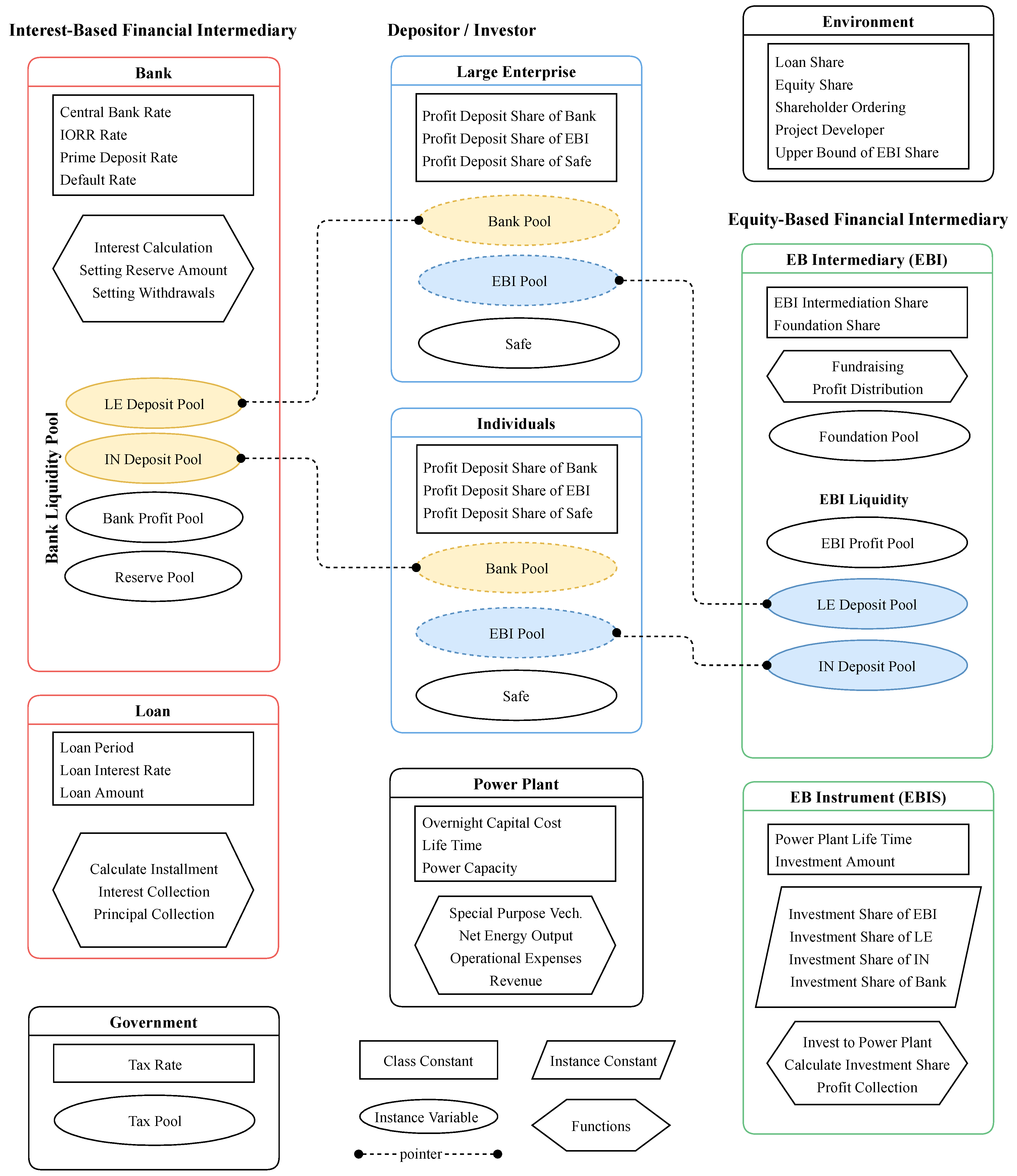
Table 1.
Wealth and Income Inequality in Nordic countries.
| Country | Date (Income Inequality) | Income Inequality | Date (Wealth Inequality) | Wealth Iequality |
|---|---|---|---|---|
| Norway | 2015 | 23.9 | 2018 | 79.1 |
| Finland | 2015 | 25.2 | 2018 | 76.7 |
| Sweden | 2015 | 26.7 | 2018 | 86.5 |
Table 2.
Configuration of the experiment on the agent-based model.
| Agent | Variable | Abbreviation | Unit | Value |
|---|---|---|---|---|
| Power Plant 1 | Overnight capital cost | OCC | QAR 2 | 766,500,000 |
| Lifetime | LT | year | 25 | |
| Construction period | CP | year | 2 | |
| Power capacity | CAP | MWp | 300 | |
| Energy yield | EY | MWh/MW | 1655 | |
| Estimated O & M cost | OMC | QAR | 29.2 | |
| Decrease rate of O&M (first yr) | DOM | - | 0.01 | |
| Rate of plant availability | RPA | - | 0.99 | |
| Degradation factor (first year) | DF1 | - | 0.03 | |
| Degradation factor (others) | DFX | - | 0.002 | |
| Land lease | LL | QAR | 0 | |
| Rate of asset management cost | RAM | - | 0.30 | |
| Rate of insurance cost | RIN | - | 0.15 | |
| Rate of other expenses | ROE | - | 0.15 | |
| Depositor/Investor | Initial capital (IN) 3 | ICIN | QAR | 766,500,000 |
| Initial capital (LE) 4 | ICLE | QAR | 1,766,500,000 | |
| Population (IN) 5 | POPIN | people | 100,000 | |
| Population (LE) 6 | POPLE | people | 10 | |
| Loan | Interest rate | LIR | - | 0.04 |
| Loan period | LP | year | 10 | |
| Grace period | GP | year | LT | |
| Bank | Central bank rate | RCB | - | 0.0225 |
| Interest of required reserves | IORR | - | 0.0220 | |
| Prime-deposit interest rate | RPD | - | 0.0105 | |
| Default-deposit interest rate | RDD | - | 0.0095 | |
| Environment | Carbon intensity (NG) 7 | CIND | g CO2eq/kWh | 46 |
| Carbon intensity (Solar) 7 | CISolar | g CO2eq/kWh | 469 | |
| Construction frequency 8 | CF | year | 2 |
Notes: 1. The inputs of power plant agent are adopted from a capstone project conducted in HBKU [52]. 2. The Qatari riyal is pegged to the US dollar at a fixed exchange rate of $1 USD = 3.65 QAR 3. This is an assumption to have this much amount of money. In this way, individuals are able to build the first power plant by their own money. 4. This assumption enables large enterprises to build the successive power plants by their own money (incorporating the profit earned from the installed power plants). 5. Gini coefficient requires the population data to calculate wealth inequality in the society. We assume a closed region, which means there is no death and giving a birth during the simulation time, with a 100 thousand individuals including micro and small enterprises. 6. According to the business population estimates [53], large enterprises constitute 0.1 percent of the population. Therefore, we assume the population of large enterprises as a ten, accordingly. 7. According to the Intergovernmental Panel on Climate Change (IPCC), which is the leading international body for the assessment of climate change, the median values of CO2 emission for solar PV farm 46 g CO2eq/kWh while those for natural gas fuel is 469 g CO2eq/kWh (excluding land use change emissions) [54]. 8. Construction frequency is the time interval between the construction of two successive power plants.
Table 3.
Policy inputs and environmental configuration of the experiment.
| Variable | Abbreviation | Value |
|---|---|---|
| Capital deposit share (pool/IN) | CDSIN, p | BANK = 1.0, EBIN = 0.0, SAFE = 0.0 |
| Capital deposit share (pool/LE) | CDSLE, p | BANK = 1.0, EBIN = 0.0, SAFE = 0.0 |
| Project developer share | DEVS | 0.15 |
| Equity intermediation share | EIS | 0.10 |
Table 4.
The summary of policy scenarios.
| Project Developer | Loan (%) | Equity (%) | Shareholder List 1 | Project Shares 2 [Shareholder Limits] | Non-Profit EBIN 3 | Foundation Share 4 | |
|---|---|---|---|---|---|---|---|
| 1 | LE 5 | 100 | 0 | (LE,Bank,IN,EBIN) | (1.0, 0.0, 0.0, 0.0) | - | - |
| 2 | LE 6 | 70 | 30 | (LE,Bank,IN,EBIN) | (1.0, 1.0, 1.0, 1.0) | False | 0.0 |
| 3 | LE 5,7 | 0 | 100 | (LE,Bank,IN,EBIN) | (1.0, 1.0, 1.0, 1.0) | False | 0.0 |
| 4 | EBIN | 0 | 100 | (EBIN,IN,LE,Bank) | (1.0, 1.0, 1.0, 1.0) | False | 0.0 |
| 5 | EBIN | 0 | 100 | (EBIN,IN,LE,Bank) | (0.20, 1.0, 1.0, 1.0) | False | 0.0 |
| 6 | EBIN | 0 | 100 | (EBIN,IN,LE,Bank) | (0.20, 1.0, 1.0, 1.0) | True | 0.5 |
| 7 | EBIN | 0 | 100 | (EBIN,IN,LE) 8 | (0.20, 1.0, 1.0) | True | 0.5 |
Notes: 1. Shareholder list implies the investor list. The shareholder list prioritizes the shareholders by assigning the agents in order (see the Section 3.2.8). 2. Project shares are only valid for a 100% loan-based scenario because project shares can be only predefined in this setting. In other scenarios, project shares can be determined by the participation shares (investment) of the shareholders in each project. Therefore, shareholder limits are valid for corresponding shareholder list in the other cases (see the Section 3.2.8). 3. Non-Profit EBIN defines the behavior of the foundation pool that is an account to deposit the excess money of the EBIN according to the investment policy. If it is false, then the EBIN is a profit-based enterprise and does not transfer any money to the foundation. 4. The details of the foundation share can be found in the subsection of the set-profit-deposit function of the EBIN in 3.1.6.1. 5. This scenario is designed for comparison purposes against the proposed models and a part of sensitivity analysis of the equity and loan share parameters. 6. This scenario is taken as a business-as-usual-case because the large enterprises (project developer) usually own the project with an average of 30% capital investment [55]. 7. This scenario is not a common practice because large enterprises, project developers, are not usually willing to invest in a project by putting in 100% of the equity. In other words, they want to employ their capital as leverage at a minimum level, thereby they usually own the project with an average of 30% capital investment [55]. However, we selected this case for comparison purposes with the 100% equity-based investments against the proposed policy. 8. This scenario is a hypothetical case because there is no such system where banking is nonexistent. However, we chose this case to show the behavior of the wealth accumulation and Gini index when banking is absent.
Table 5.
Results of the seven policy scenarios.
| Results | Policies for Comparison | Proposed Policy Implications | |||||
|---|---|---|---|---|---|---|---|
| Scenario 1 | Scenario 2 | Scenario 3 | Scenario 4 | Scenario 5 | Scenario 6 | Scenario 7 | |
| WA—Bank (QAR in Billions) 1 | 15.078 | 12.056 | 5.401 | 4.135 | 3.684 | 3.712 | 0.00 |
| WA—EBIN (QAR in Billions) | 0.00 | 1.792 | 4.318 | 19.346 | 12.296 | 2.636 | 2.636 |
| WA—LE (QAR in Billions) | 11.352 | 14.211 | 23.446 | 4.573 | 5.476 | 5.682 | 4.212 |
| WA—IN (QAR in Billions) | 1.230 | 1.23 | 1.23 | 4.027 | 10.041 | 10.041 | 9.343 |
| WA—FND 2 (QAR in Billions) | 0.00 | 0.00 | 0.00 | 0.00 | 0.00 | 9.482 | 9.482 |
| WA—Total (QAR in Billions) | 27.66 | 29.289 | 34.395 | 32.081 | 31.497 | 31.553 | 25.673 |
| Gini Index | 0.955 | 0.958 | 0.964 | 0.874 | 0.681 | 0.483 | 0.311 |
Notes: 1. The WA stands for Wealth Accumulation. 2. The FND stands for foundation.
© 2019 by the authors. Licensee MDPI, Basel, Switzerland. This article is an open access article distributed under the terms and conditions of the Creative Commons Attribution (CC BY) license (http://creativecommons.org/licenses/by/4.0/).
Share and Cite
MDPI and ACS Style
Ari, I.; Koc, M. Sustainable Financing for Sustainable Development: Agent-Based Modeling of Alternative Financing Models for Clean Energy Investments. Sustainability 2019, 11, 1967. https://0-doi-org.brum.beds.ac.uk/10.3390/su11071967
AMA Style
Ari I, Koc M. Sustainable Financing for Sustainable Development: Agent-Based Modeling of Alternative Financing Models for Clean Energy Investments. Sustainability. 2019; 11(7):1967. https://0-doi-org.brum.beds.ac.uk/10.3390/su11071967
Chicago/Turabian StyleAri, Ibrahim, and Muammer Koc. 2019. "Sustainable Financing for Sustainable Development: Agent-Based Modeling of Alternative Financing Models for Clean Energy Investments" Sustainability 11, no. 7: 1967. https://0-doi-org.brum.beds.ac.uk/10.3390/su11071967
Note that from the first issue of 2016, this journal uses article numbers instead of page numbers. See further details here.