1. Introduction
Sustainability in the context of railway operation is a multidimensional aspect. Train operators are interested in efficiency in terms of the availability and access costs of railway infrastructure, while users of railway services place emphasis on transport punctuality/reliability or speed [
1]. Moreover, in most countries, governments pay large subsidies for railway infrastructure and passenger transport. In these cases, the focus of the government is in asking if those subsidies are spent efficiently, or how, through higher efficiency, they could be reduced [
2].
In the last few years, railway-traffic optimization has had increasing interest. The number of users and trains on railways have grown, while the capacities of railway stations have not increased in the same fashion, usually due to limitations of areas in which they are located. Railways can offer high capacity, sustainability, and low energy consumption, but require a more efficient use of resources and the application of more advanced decision tools.
The objective of this paper was to model the scheduling of trains on a railway network as a Mixed Integer Linear Program and develop a heuristic algorithm to optimize scheduling. The motivation of this work was train scheduling, but other situations may fit in the same mathematical model.
Some operators like Schweizerische Bundesbahnen (SBB) are investigating the possibility to automate the process [
3]. In general, there is an increasing interest from the railway industry in this direction to guarantee quality of service and efficiency.
The situation addressed in this work is that of a network composed by busy multiplatform stations that are composed of a number of tracks served by footpaths fit for passengers or freight services, connected by at least a one-way track in each direction, which is the most common situation around Europe. Scenarios, more common in North America or Russia, where there are far stations connected by one two-way track with loops for the intersection of trains in opposing directions, are out of scope of this paper. Although the solver may be able to also manage this situation, there is a fair amount of research that specifically addresses it [
4,
5].
The task of scheduling trains on a network is an evolutionary process. Thus, there is almost never complete redesign, but the new timetable is based on the previous one with some variations or adjustments. Some networks are operated on a clock-face schedule, and they have traffic so dense that respecting the clock-face structure is a priority. The Swiss railway network, for instance, has been adapted in such a way that the journey time between main stations is a multiple of 30 min.
Another key point to consider that is common in Europe is international traffic that is usually decided before internal traffic and becomes a constraint of the problem.
Scheduling means generating a timetable that gives arrival and departure times for each train at various points on the network. The difficulty in this process is given by the fact that it is necessary to take into account possible conflicts between trains over a resource that can be, for instance, a crossing between two ways. The objective of scheduling is to avoid such conflicts in the planning phase by computing the time instants in which each train should take over and release a certain resource.
The main difference with other kinds of algorithms that can be employed for packets or other kinds of vehicles and infrastructure is the fact that trains cannot overpass one another, and that it is not possible to buffer them. This means, in other words that if the entrance of a train into a section is delayed, then the section before is occupied for a larger amount of time, and no other train is allowed into or through it.
Another purpose of the algorithms is that they can be used to simulate and explore the effects of alternative draft timetables, operating policies, station layouts, and random delays or failures.
In a feasible timetable, all train paths have to respect timing constraints, interaction constraints, safety-regulation constraints, and commercial constraints. There are various objective functions that can be used. In this paper, the objective was to minimize the sum of delay times of all trains. This objective function was chosen as operators often want short run times, and the objective also promotes efficient capacity utilization, as trains spend as little time as possible on the tracks.
In the context mentioned before, delay-aware scheduling becomes vital for efficient resource assignment in complex railway scenarios, improving the level of safety and punctuality. These terms relate railway sustainability that is increasingly socially demanded to the reliability and availability of the solution. To this aim, in this document, we present the mathematical modeling of the problem along with a solution strategy, where the main contributions are:
Development of an original mathematical formulation as a mixed linear optimization problem of the complex system, including the microscopic detail of railway-service requirements. The model obtains optimal solutions improving this computation time of some results published in the literature in similar scenarios, and is scalable in the sense that the computation time is independent of the number of train requests;
heuristics based on genetics able to generate good-enough timetables for a large geographical area and many trains with multiplatform stations. With this algorithm, optimal or near-optimal solutions can be quickly computed in a reasonable execution time, improving others’ published alternatives solutions; and
performance evaluation of the results of this work comparing with other literature solutions. Moreover, a study of the sustainability of our proposal is included, analyzing how does it work keeping a constant number of train instances and reducing the number of platforms in the stations, being a more sustainable solution. Here, sustainability refers to the ability of maintaining the existing railway infrastructures while the traffic of trains increases, requiring better utilization of the resources. Avoiding increasing the infrastructure can improve sustainability by reducing the maintenance costs.
Thus, the goal was to optimize the railway schedule and simultaneously provide tools to obtain results in an efficient way and acceptable execution times.
Research for this study was conducted in four main steps: (i) literature review focused on train scheduling on railway networks composed of busy complex stations; (ii) design of a mathematical model including the complexity of the scenario; (iii) providing heuristics based on genetic algorithms to solve the problem; and (iv) evaluation of both proposals applied on the request of a real railway operator, compared with other solutions.
The remainder of this work is organized as follows:
Section 2 presents the literature review.
Section 3 describes and formulates this specific train-scheduling problem, including the parameters, variables, objective function, and constraints.
Section 4 describes the heuristics based on genetics implemented to solve the problem in reduced computation time by using the tools presented in
Section 5. The model and heuristics are tested and analyzed in
Section 6 in a real-life situation at railways proposed by the Swiss Federal Railways. In
Section 6, we also included a comparison with other literature proposals and the measurement of a parameter related to sustainability. Finally,
Section 7 concludes the work and points out future directions for research.
2. Literature Review
Scheduling trains on a railway network is known to be an NP-hard problem with respect to the number of conflicts [
6,
7].
The benefits of using optimization to generate timetables has attracted many research efforts on optimization models for the train-scheduling problem [
8,
9]. In this context, some works [
10,
11,
12,
13,
14,
15] presented surveys on railway optimization. Specifically, the work in [
12] provided an overview on train routing and scheduling, authors in [
13,
14] dealt with passenger transportation, and authors in [
15] presented the main works on train timetabling and train routing.
In [
16], the authors studied the joint problem of scheduling passenger and freight trains for complex railway networks with the objective of minimizing the tardiness of passenger trains at station stops, and the delay of freight trains. They provided an MILP and proposed two-step decomposition heuristics to solve the problem.
The majority of the proposed mathematical optimization models become impractical when trying to solve the timetabling problem for large geographical areas and many trains. However, since the advent of computers, people started to think about ways to automatize the process and develop heuristics to find and solve conflicts in polynomial time.
Nedeljkovic and Norton [
17], for example, developed heuristic techniques for Westrail to generate master train schedules recognizing the relative priorities of trains. The method heavily relied on man–machine interactions.
Remaining in Western Australia, Mees [
18] presented an efficient approximate algorithm that could quickly find good feasible solutions for real-world networks with modest computing resources.
Cai and Goh [
19] proposed an algorithm that was based on local optimality criteria in the event of a potential crossing conflict. A suboptimal but feasible solution could very quickly be obtained in polynomial time. The model could also be generalized to cater for the possibility of overtaking when trains have different speed.
Higgins et al. wrote a series of studies in the field, employing branch and bound [
4] and various local search heuristic techniques [
5] for scheduling on single-line rail corridors.
Carey and Crawford [
20] proposed a heuristic technique to solve the problem of scheduling trains on a network of busy complex stations, like the ones that can be found all around Europe.
Genetic algorithms [
21] were successfully employed in the solution of complex scheduling problems. Under the assumption that genetic algorithms are suitable for the addressed problem, a solver was developed, employing genetic-algorithm implementation. Some recent studies applied genetic algorithms in the field, for example, to reduce the number of trains subject to a given passenger flow [
22], or to assign drivers to trains [
23].
Finally, Tormos et al. [
24] developed a genetic algorithm for railway-scheduling problems that were used to solve real-world instances with good performance. Arenas et al. [
25] developed and compared a mathematical model and a genetic algorithm showing that, in some cases, the model solver outperformed the heuristic. Likewise, Wang et al. [
26] proposed a mixed integer programming model to address the timetable-rescheduling problem, considering strategies such as retiming, reordering, and adjusting stop patterns applied in a Beijing–Shanghai high-speed railway corridor. A genetic algorithm-based particle-swarm optimization algorithm was developed in this work. However, the proposed model did not consider longer disruption lengths.
In this context, this work tries to further explore the possibilities of applying parallel genetic metaheuristics with real-time concurrency to train scheduling, which produces better and more robust results, and more optimal individuals than a nonparallel one, solving larger problem instances in a reasonable computing time [
27].
Related to sustainability, Kapetanović et al. [
28] presented an interesting analysis of the contributions in environmental sustainability related to passenger railway services.
3. Mathematical-Model Formulation
The overall aim of this mathematical model was to produce a conflict-free timetable for all trains running on a railway, with complex multiplatform stations consisting of a set of parallel tracks. Links that connect these stations can either be single-track or multitrack sections.
The travel information of a train is modeled by continuous time variables and binary assignment variables. Continuous time variables identify the time when the train enters or leaves a section of a path. These values are constrained by functional requirements that force paths to be within a predefined period of time, such as earliest departure time, latest arrival time, minimum stopping times, and connections to other trains. There are also technical limitations to this scenario, i.e., a set of routes it could take from origin to destination, together with minimum running times on the sections and a list of resources that are occupied while the train is in a section. Trains can only stop at certain stations and, if this happens, running time in the preceding and succeeding sections must be increased due to speed variation. In addition, the interaction of two or more trains in the case of trying to use the same resources at the same time was modelled using binary interaction variables.
With all of this information, the mathematical model had produced a timetable with the assignment of a continuous time instant to each event that did not violate any functional and physical requirements, and did not result in resource-occupation conflicts.
The presentation of the model starts with the introduction of notations. Then, the meaning of the employed parameters and variables is explained. Finally, the objective function and constraints are introduced and discussed.
3.1. Subscripts and Superscripts
The following superscripts are used in the article:
in, indicating a parameter or a variable related to the entrance in a section; and
out, indicating a parameter or a variable related to the exit from a section.
Subscripts indicate an index that can vary in a set.
3.2. Parameters
First, information about routes and service intentions (SI) is read from input files. A service intention represents a railway service that has to be scheduled on the network according to a draft timetable, while a route describes all alternative paths that a train can follow to move between scheduled stations. In this context, terms ‘SI’ and ‘train’ are used indistinctly.
Route information includes an ID and a list of route sections, each with values related to:
minimum running time, mrt;
minimum stopping time, mst;
penalty in case of using route section by a service intention, p;
earliest/latest entry/out times, EarIn, EarOut, LatIn, LatOut;
entry/exit delay weights, win, wout;
release time or minimum time to wait for coincidence between two SIs at a common section R; and
route alternatives between source and destination.
Minimum running time of a route section, mrt, is the minimum time duration the train must spend on that route section. The scheduled stop time of a train in a station consists of minimum stop time, mst, for necessary operations permitting passengers to safely get on or off the train, and of additional buffer time to take into account the possible way time in traffic or scheduled connections.
The international union of railways (Union International des Chemins de fer, UIC) produced a series of recommendations (UIC leaflet 451-1 OR) in regard to the implementation of running-time supplements in timetables based on empirical data [
29]. The UIC recommends the use of a fixed minimum-running-time supplement for all railway traffic, and an additional speed-dependent percentage running-time supplement. In this work, in order to simplify and without losing generality, these supplement times were assumed to be included in the minimum running time and release time.
If a section requirement specifies entry latest (LatIn) and/or exit latest (LatOut) time values, then the times for the entry and/or exit events on the corresponding train-run section should be less than the specified time. If the scheduled time is later than required, the solution is still accepted, but it is penalized by the objective function using Entry (win) or Exit (wout) delay weights.
On the other hand, if a section requirement specifies entry earliest (EarIn) and/or exit earliest (EarOut) time values, then the times for the entry and/or exit event on the corresponding train-run section must be greater than the specified time.
Using this information, all feasible paths for each service intention were computed taking into account all alternatives. This set of paths was modeled as a directed acyclic graph.
In order to manage service intentions, routes, and sections, different sets were defined as parameters of the model. Thus, there is a list of SIs, a list of paths for each SI and a list of the resources of each path of each SI. There is also a general list of route resources:
- SI
Set of Service Intentions. This is the list of train demands required in the problem.
- P
Set of Paths of each SI, taking into account alternative paths. Each element of this set depends on the service intention, si, and one feasible route of the si, r. Thus, the set of indexes of one element of P is (si, r).
- RS
Set of Route Sections of each path of each SI (counting alternative paths). Each element of this set depends on the service intention, si, one feasible route of the si and one route section of this path, rs. Thus, the set of indexes of one element of RS is (si, r, rs).
- RE
Set of Resources feasible to be used by each SI. Each element of this set depends on the service intention, si, and one feasible route section to be used by it, re, i.e., the set of indexes of one element of RE is (si, re).
- RSE
Set of Resources of each SI at each route. Each element of this set depends on the service intention, si, one feasible route of the si, and one section of whatever path of the list of resources, re. Therefore, the set of indexes of one element of RSE is (si, r, re).
- RSI
Set of pairs of service intentions and possible resources to be occupied by them. Each element of this set depends on the pair of service intentions, si1, si2, and one section of the list of resources, re. Thus, the set of indexes of one element of RSI is (si1, si2, re).
- RSIRE
Set of pairs of service intentions, their routes, and possible resources to be occupied by them. Each element of this set depends on the pair of service intentions with feasible routes, si1, r1, si2, r2, and one section of the list of resources, re. Therefore, the set of indexes of one element of RSIRE is (si1, r1, si2, r2, re).
In addition, we defined M and for linearization purposes, being M a large-enough constant, and a small-enough positive value to ensure that violating a linearized constraint is never optimal.
3.3. Variables
The following are the real-time variables defined in the model for each service intention (SI or train) occupying a resource
of a route
r:
Continuous time Variables (
1) and (2) are the result of our model, representing a timetable with the assignment of a continuous time instant to each event, i.e., trains entering or exiting a section of a path.
In addition, the following binary variables allowed us to determine when a service intention uses a route or occupies a section of a route without collisions with other trains:
Using Variables (
3), a unique path is selected for each service intention (train). Variables (4) determine which resources are finally used for a service intention. The last set of Variables (5) is used for avoiding collisions between two trains passing through the same section (either the same path or not).
3.4. Objective Function
The objective function of this problem was to minimize total train delay. Delays are positive deviations between realized times and scheduled times of arrival and departure times of the route sections. In general, delays could be classified into (i) delays due to the variability of process times, e.g., equipment failures and large passenger flows; and (ii) delays that are originated because trains have to be queued by dispatching decisions due to sections only being able to be occupied by one train at the same time [
30]. All of these delays were included in our proposal. Other delay causes, such as train or infrastructure failures, are outside the scope of this paper [
1].
Thus, the way to measure the goodness of a solution is the weighted sum of all train delays. The delay is zero if all trains are scheduled such that they arrive at each of their defined stops no later than desired. This problem also includes the possibility that a route or some routes for a train are more desirable than others. In this way, if an undesired route is chosen, the solution incurs an additional “routing penalty” that increases the objective-function value.
Therefore, the objective of the optimization was to minimize the delay of each train and, at the same time, avoid using some tracks if possible. Thus, this is a multiobjective problem that could be modeled by cost Function (
6) using the Goal Programming method:
The first term of Function (
6) is the weighted summation (using weights
and
) of the difference between current entrance time into a section of a train and its desired latest entry time in this section (
), plus the difference between current exit time from a section and its desired latest output time of this section (
).
Weights allow for the greater or lesser prioritization of entry times in a section of the route compared to departure times. On the other hand, the maximum operation in the first term avoids an early train giving a negative contribute to the objective value.
The second term of Function (
6) includes the summation of all penalties due to selecting routes with lower priority. In this formulation, the priority of a service is encoded into the weight of the corresponding delay, i.e., a service with higher priority has higher weights than one with a lower priority.
3.5. Constraints
It is necessary to respect several constraints to obtain valid solutions. First, constraints that define the behavior of one train along the sections of a route to ensure a comfortable railway service. This means avoiding a train departing earlier than the scheduled departure time, avoiding the stop being short to let passengers safely get on or off the train, or avoiding the scheduled connection between two trains being too short for passengers to effectively take advantage of it.
The first set of Constraints (
7) specify that, if
, i.e.,
r is the selected path of a service intention or train
; the minimum time between entering and going out of a section of this path is the summation of the minimum running time and the minimum stop time:
Constraints (
7) with (
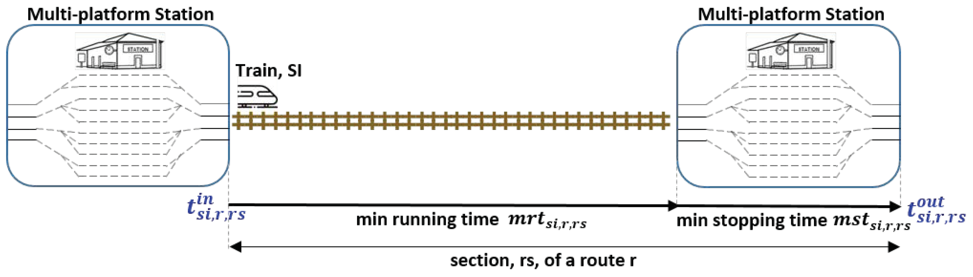
8) determine the sequence of times along the sections that form the route to be used by the service instance, as it is shown in
Figure 1 (the train first enters into the section and then goes out). Moreover, constraints in (
9) define that each track section is occupied right after the section before it is freed. In others words, after a train frees one section, it does not get lost, but immediately goes in the next railway section:
Applying linearization procedures, Constraints (
7) are formulated as follows (
10), being
M a constant value big enough to include the remaining time of a train inside the farthest section of all paths, i.e.,
:
The next constraints specify the earliest requirements for the selected path of each service intention, i.e., if
. The first set of Constraints (
11) avoids earlier departure than the scheduled departure time, and the second set of Constraints (
12) avoids stopping not long enough in the station for the passengers to safely get on or off the train:
Linearizing Constraints (
11) and (
12), the following formulations were obtained (
13), (
14), being
M greater than or equal to the greatest earliest entry or out time:
In addition, Constraints (
15) ensure that exactly one path is assigned to each service intention:
On the other hand, Constraints (
16) establish the relationship between variables
and
, i.e., if a route r is assigned to a service intention, all sections of this path are occupied by this service intention (train):
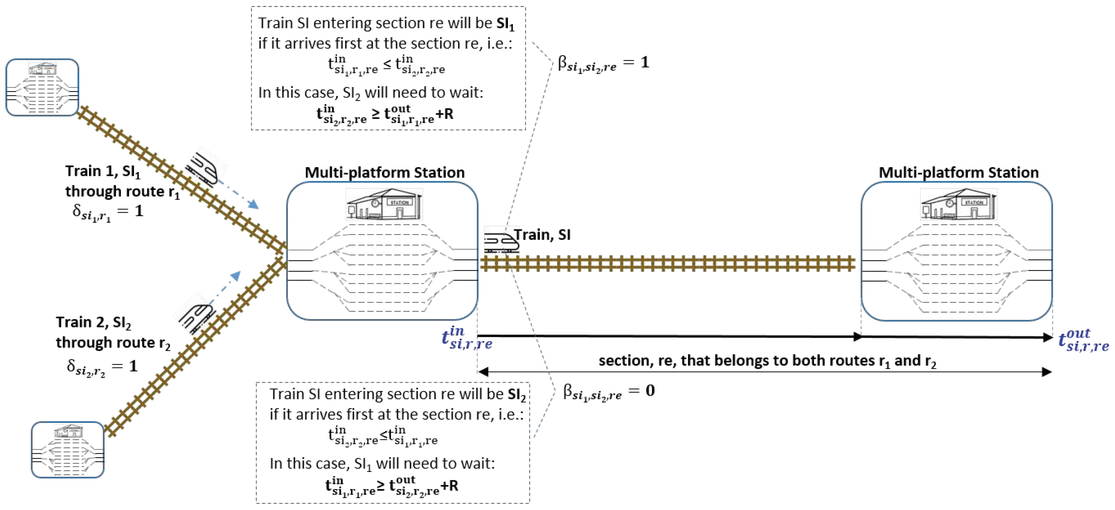
Finally, the following constraints solve the coincidence at a common section of two service intentions. Conditions that were linearized in the model related to collision avoidance are the following. First, we needed to determine the values of binary variables
with the conditions of (
17). In the case of two service instances (trains)
,
, having been assigned different routes,
(
) and
(
) sharing a common section
(
), if Train 1 arrives earlier to section
than Train 2, then binary variable
is equal to 1. In the opposite case, if Train 2 enters section
earlier, then
is equal to 0:
As a consequence, depending on the value of
, one train is delayed to avoid collisions in the shared section (see (
18)). The sequence of time events in this case of coincidence of two trains at a common route section is shown in
Figure 2:
By means of linearization procedures applied to (
17) and (
18), Constraints (
19)–(
22) can be obtained.
Constraints (
19) permit fixing
in the case of two selected paths for service intentions
and
(
and
, respectively), coinciding at section
, and
entering earlier than
. In the same way, Constraints (
20) establish
in the case of two selected paths for service intentions
and
(
and
, respectively) coinciding at section
, and
entering later than
:
and for both constraints
.
Constraints (
21) determine that, in the case of section coincidence and
, the second train (
) entry time to the section has to be delayed until the first train (
) has left the section plus an extra time R (time to wait between two trains that share a common section to avoid collisions). On the contrary, Constraints (
22) provoke the delay of the first train:
and for both constraints
.
This model was implemented using Python-based package Pyomo [
31,
32] with Gurobi as the underlying solver [
33].
4. Heuristic Solver
The mathematical model of the problem is an integer optimization problem with side constraints, and it is difficult or impossible to solve exactly in a reasonable amount of time. In order to solve this NP-hard problem, a heuristic approach was implemented that makes use of genetic algorithms to find a good solution.
The program reads the input files, generates an instance data structure containing both the list of resources and the routes with the corresponding indication of the section requirements, and feeds the genetic-algorithm framework. This uses the instance to generate a number of solutions that compose the initial population, and to combine these solutions with the single-point crossover technique to improve the objective value of the solution.
The full implementation of the program developed to solve the train-scheduling problem is discussed in this section, starting from the input and output model, to describe the data structures used internally, the resource manager used to ensure coherent resource management, the algorithm used to produce an individual of the initial population, that is, a solution generated with a certain amount of randomness, to the techniques employed in genetic optimization.
4.1. Input and Output Model
The input files consist of json serialized structures that represent service intentions, routes, and resources.
The service intention is an ordered list of section requirements. Because json serialization and deserialization do not guarantee keeping ordering correct, each entry contains a sequence number.
The section-requirement object encodes information about the earliest and latest instant at which a train is expected to enter and exit a station or a certain block, the minimum duration of the stop at a station, and the weight of a delay after the latest intended entry or exit of the train into the required section. All information is optional. Moreover, it can contain connections with other service intentions. In this case, the connection structure indicates how much it should last in order to allow passengers to comfortably change services.
Each service intention is linked through a unique identifier to a route, that is, a directed acyclic graph represented through its edges that are the route sections. The graph is divided into route paths, linear subgraphs that represent alternative paths a train can take, for example, different ways into a multiplatform station. Edges in each route path are connected in sequence, and route paths are connected to each other using markers, i.e., unique strings that identify nodes.
Each route section contains the list of resource identifiers that a train would require when occupying the section, and the minimum time required for the train to pass through the section. An optional section marker allows the link between section requirements and route sections.
Finally, resources are identified by using a string that contains a release time. Some resources could allow following trains in the same direction to pass through before the release time has expired.
The output of the program is a json file. The main object is a solution that contains a label and a hash that identify the problem instance, a hash that assures integrity of the solution file, and a list of train runs. Each train-run contains the identifier of the service intention and of the route into the problem instance, and a list of train-run sections. A train-run section indicates the time of entrance and of exit from the route section and the identifier of the route section itself, plus a sequence number to preserve the correct ordering and the section marker if the current section is a requirement.
The structures derive the Serialize trait and are automatically converted into valid json strings by the serde-json library.
4.2. Internal Representation
After the input file is deserialized, it must be converted into a more suitable representation. Each service intention and the corresponding route are merged into a unique data structure that is a graph. Each node of the graph is an “event” that contains optional time that is left unassigned in the first place, and an optional marker, if this is assigned by the “route_alternative_marker_at_entry” or “route_alternative_marker_at_exit” fields of the route section. The edges of the graph instead bring all information about the route section, and to the section requirement if the current route section corresponds to a section requirement.
A vector contains the source points and is associated with the graph into the “Route” struct. The set of the graphs obtained in this way, collected into a wrapper struct called “Route Manager” and the set of the resources taken directly from the input model, constitute the internal representation of the problem instance: a struct called “Instance”.
A resource manager is created from the list of resources every time a solution must be generated or checked.
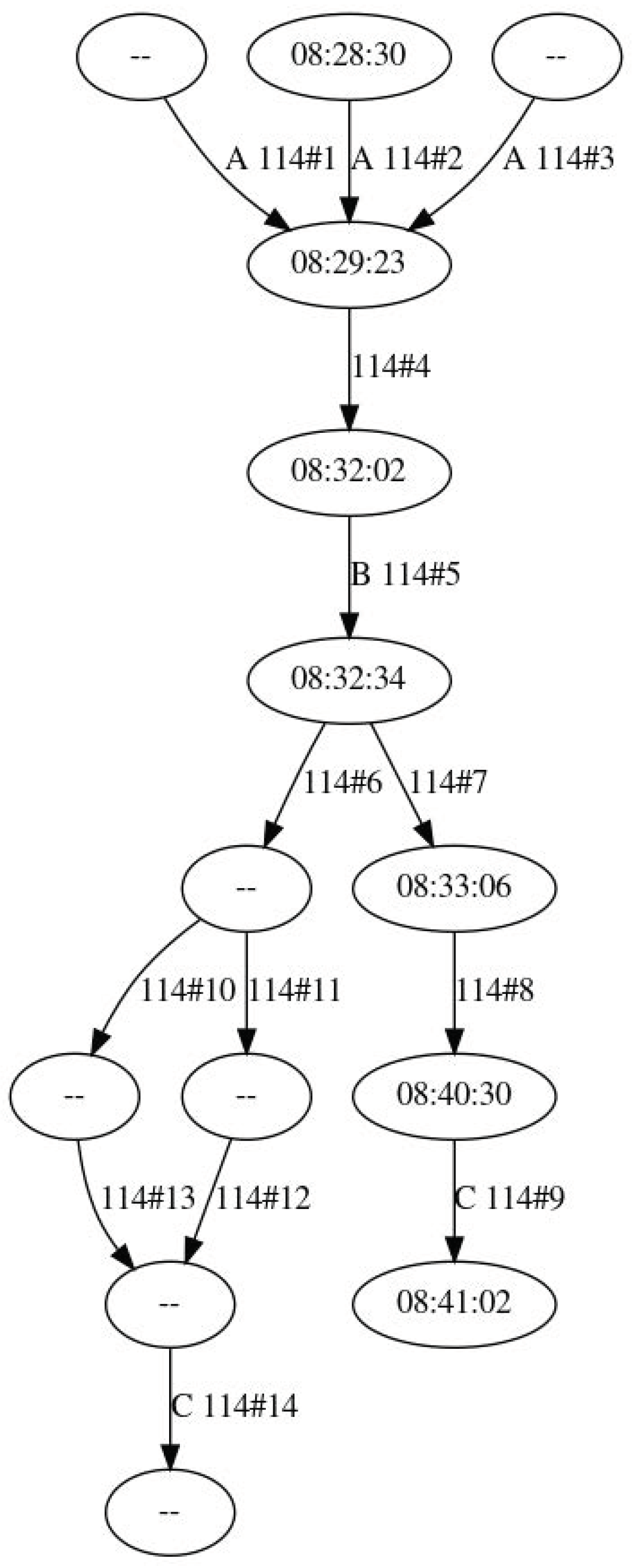
After a service intention is scheduled, it produces the internal representation of a “TrainRun” that is a graph similar to the one in the instance, but with all times assigned on the chosen path. For convenience, there is also a vector containing the sequence of nodes of the chosen path and another containing the related times. The service-intention id is also kept associated with these structures. The collection containing all “TrainRun” is the “Solution” of the problem.
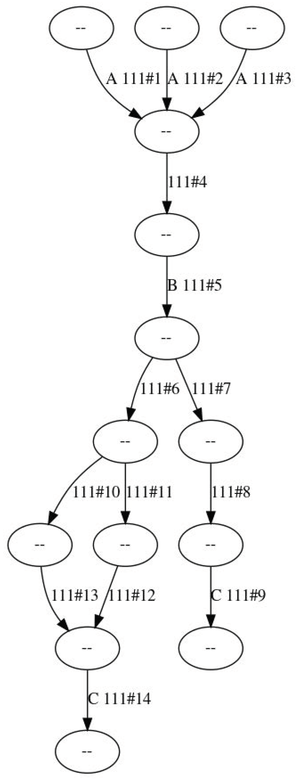
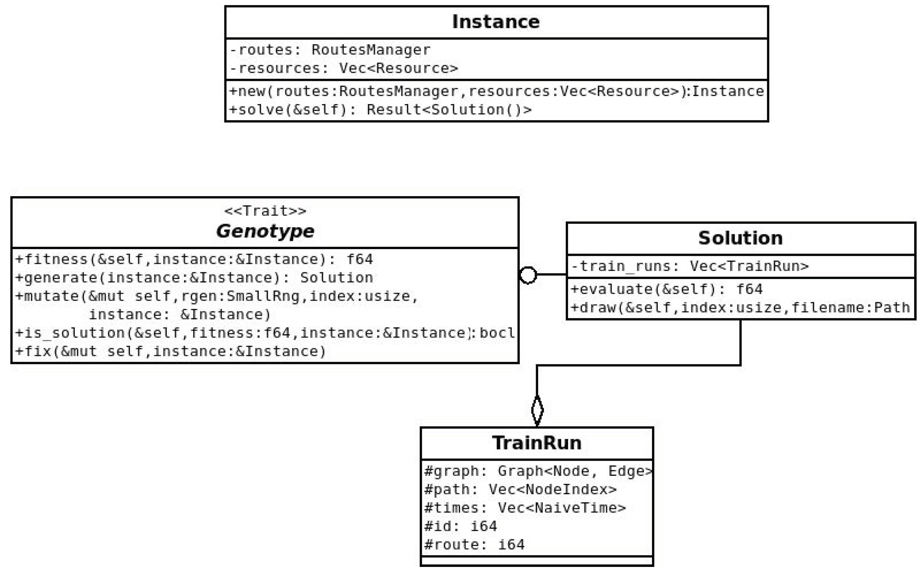
Figure 3 shows how the generated graph looks like in a very simple case, while the Unified Modeling Language (UML) class diagram in
Figure 4 illustrates the definition of the data structures. This representation is optimal to compute the value of the objective function or to perform further optimizations, but it has to be converted into a more suitable one before being emitted as output. The struct also implements the “Genotype” trait providing methods for genetic optimization.
4.3. Resource Manager
From the list of resources, a HashMap is generated that allows direct access to a resource. The values are protected by a Mutex lock to allow for safe and concurrent resource allocation. In the values, an interval vector keeps track of the allocations. A wrapper object built around the map provides safe resource management, allocating time intervals and considering the release time needed by each resource.
The vector containing the allocation intervals works like an interval tree, allowing only the insertion of nonoverlapping intervals, and refusing other cases.
The “Interval” struct contains the identifier of the service intention and the index of the route section that allocates the resource for the interval. It also contains the start and end instants.
Ordering operation (“Ord” trait) is implemented for this struct based only on the start field. This allows for easier and more efficient management of the consistency of this structure. In fact, to see if an interval has collisions, it is sufficient to perform a binary search into an ordered vector: if the search is successful, the result is the exact position of the first colliding interval; otherwise, the first colliding interval may be the one before the position where the new interval should have been, the one in that position, or both. One of the two may not exist and, in either cases, only one comparison is needed.
Private method “search_collisions” returns the range of intervals colliding with a given interval on the given resource. The resource mutex must be locked before calling the method, and the lock is passed to it. This functionality is exposed by the “collisions” public method that returns a vector with all intervals in the range.
The “take” method instead uses it internally to verify that a request is acceptable. This function accepts allocations that collide with intervals scheduled by the same intention; it returns an error if the requested resource does not exist, if the requested interval has a negative duration (i.e., the end precedes the start), or, if there is a collision, specifying the first collision with another intention. On a success, a token is instead returned containing a reference to resource and interval that allows easy resource deallocation.
An extensive test suite was developed for this data structure to find and fix bugs, as it is the core of the entire heuristic algorithm.
This structure heavily exploits cache locality, as all intervals are stored in a continuous memory space, but insertion requires the copy of the intervals that are located after the insertion point. Another possibility would have been to base it on a Tree or B-Tree structure, but it was not already available in the Rust ecosystem, and its development is outside the scope of this work. Moreover, it could have also had worse performance because of the impact of cache locality on the vector, and the capability of modern computers to copy large portions of memory very quickly.
4.4. Generation of Initial Population
Each individual of the initial population is generated according to the algorithm described in this section. This corresponds to the “generate” method of the genotype interface illustrated in
Figure 4. The algorithm produces a feasible solution that tries to be good but not optimal. Some randomness ensures that the initial population is wide enough.
The algorithm was designed to be partially concurrent so that it can easily scale out on more complex problems, using more pieces of hardware instead of more expensive ones.
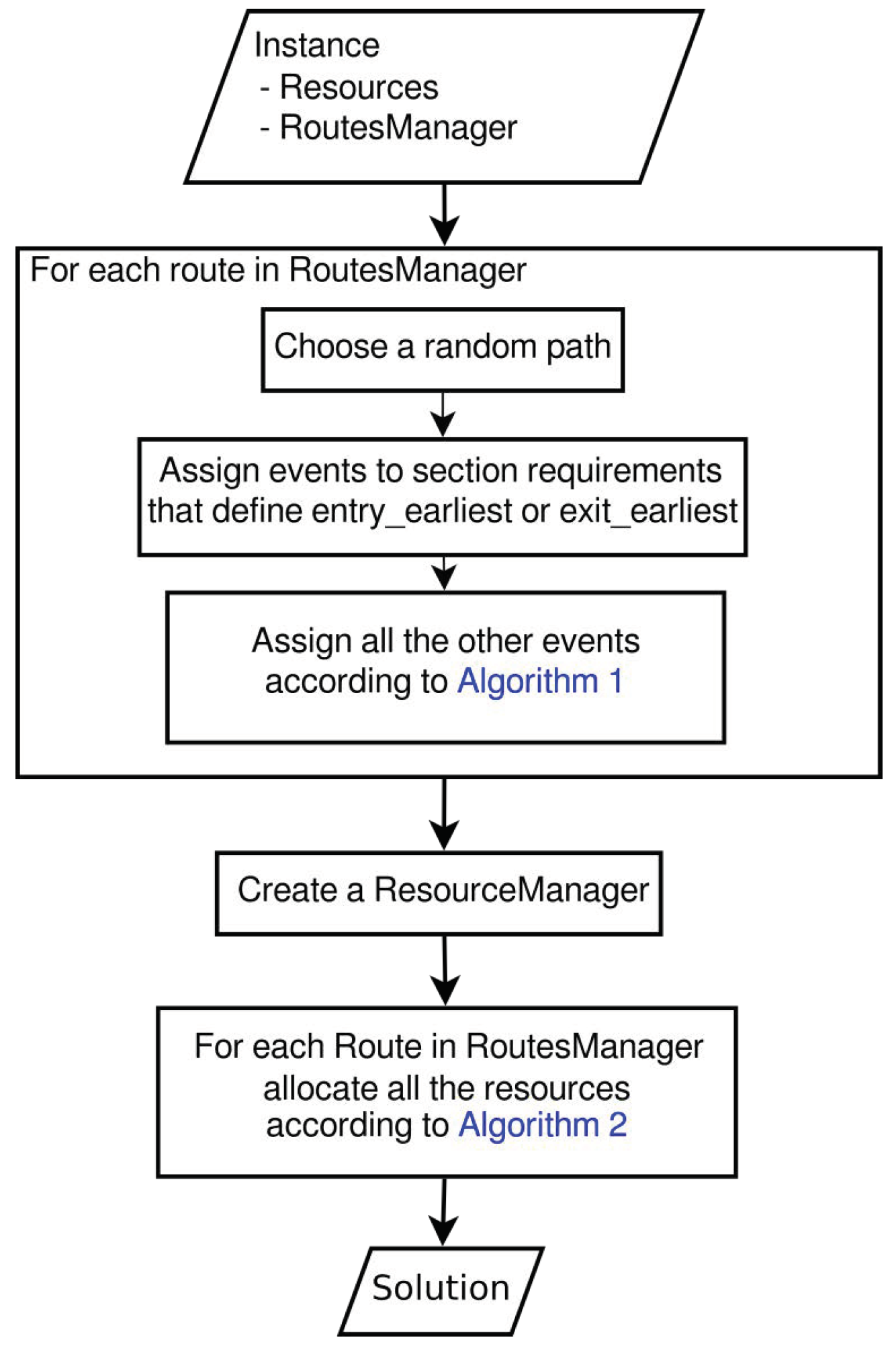
The algorithm takes as input an instance structure and generates a solution structure. To do this, for each route in the RouteManager, a random path is chosen, time events are assigned, and resources are allocated.
Figure 5 illustrates the main steps of the algorithm in a block diagram; they are examined in depth in the follow-up.
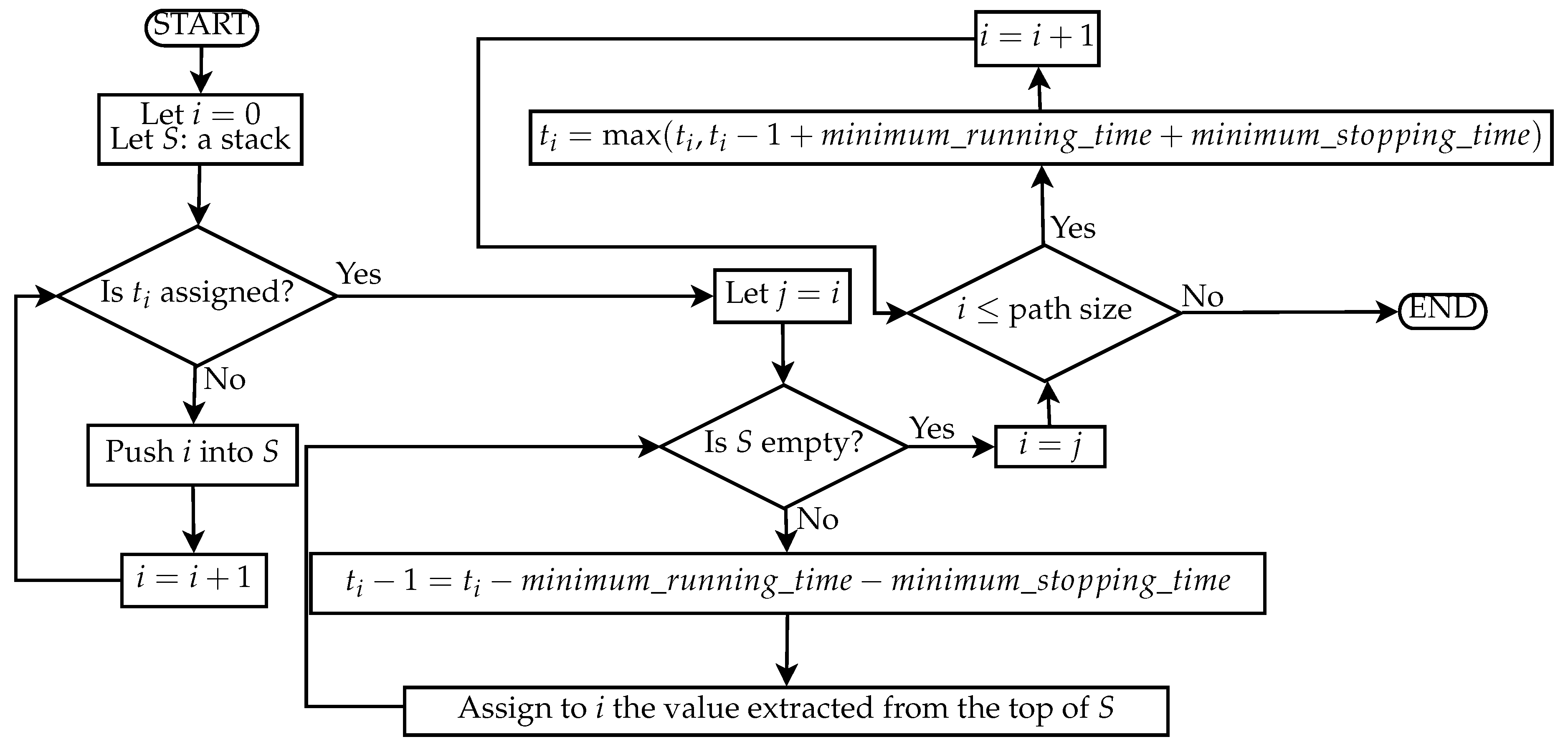
The first step is to chose a path and compute a feasible timetable for this path. When there are alternative paths, one is chosen randomly without considering that some paths incur in penalties. At this point, some of the events are assigned based on the section requirements that set an entry- or exit-earliest rule. The other events are instead assigned according to the strategy of Algorithm 1 illustrated in
Figure 6 in the form of a flow chart.
| Algorithm 1 Event assignment considering mrt and mst |
|
| while is None do |
| |
| |
| end while |
|
| while not stack.is_empty() do |
| |
| |
| end while |
|
| while i <= path.size() do |
| |
| |
| end while |
Considering that the maximum between a nonassigned instant and another is never the unassigned, this operation ensures that we do not introduce unfeasibilities that violate Functions (
13) or (
14).
This part of the algorithm is performed in parallel on the base of the service intentions: each service intention is treated as a separate job and actual concurrency use the technique of work stealing to avoid the unequal division of the work between physical processing units.
At this point, all the constraints except resource allocation and the connections between services are enforced by construction.
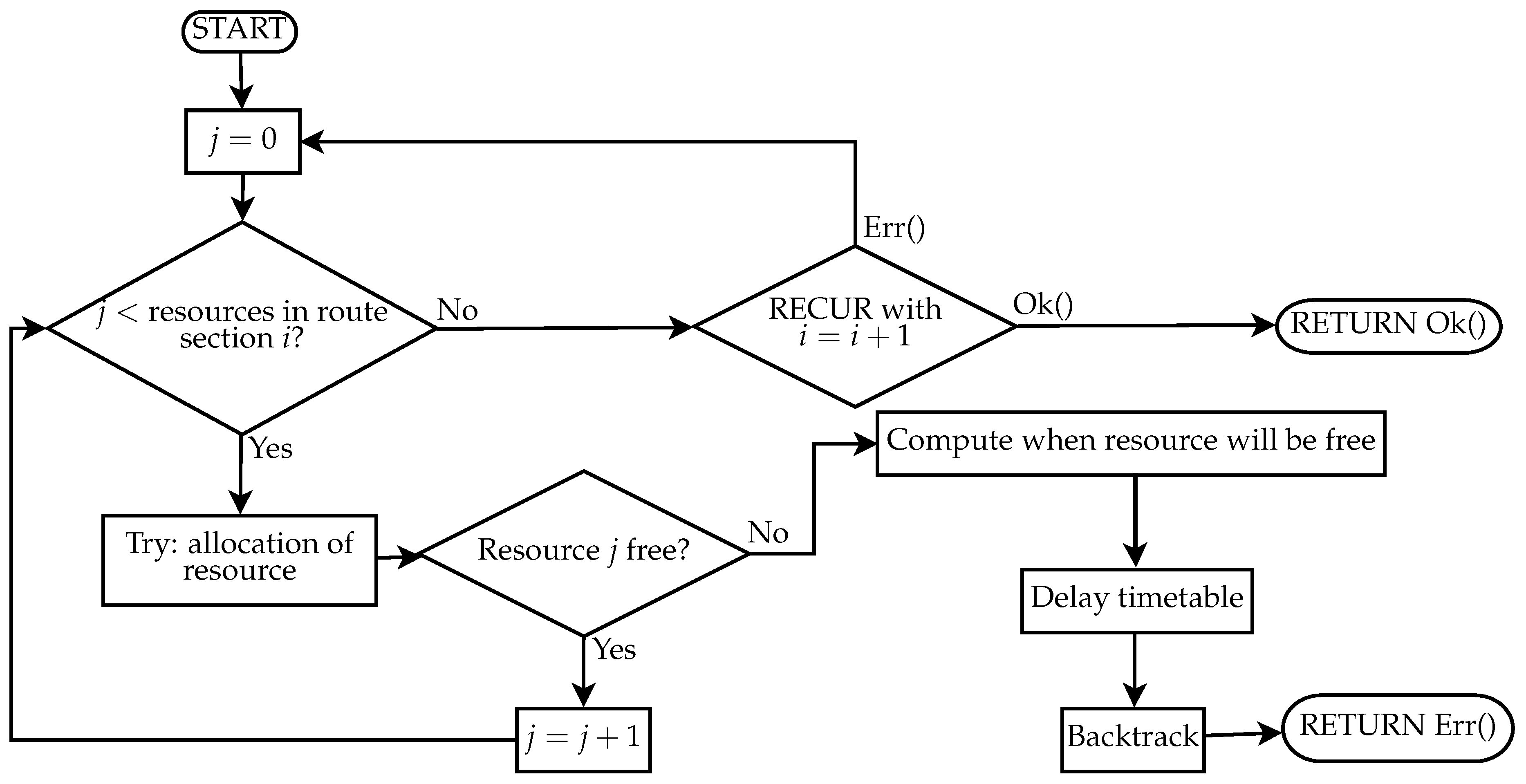
The next step of the algorithm is resource allocation. This is done in a separate method as it is also used to fix unfeasible solutions resulting from the crossover of other solutions in the genetic metaheuristic framework.
To perform it, a new resource manager is created. Then, for each service intention, a recursive allocation function is called until it returns with success. The pseudocode in Algorithm 2 and the flow chart in
Figure 7 show how it works.
| Algorithm 2 Pseudocode of recursive function responsible for resource allocation. |
| loop |
| for all resources in route section i do |
| try allocation |
| if Occupied then |
| Compute when resource become free |
| Delay the timetable |
| Backtrack |
| Return an Error |
| end if |
| end for |
| Recur with |
| if Ok then |
| return Ok |
| end if |
| end loop |
The call after the last section returns OK and terminates the recursion. Resource allocation is done in a sequential way to avoid repetitive conflicts on a resource by services that happen to occupy some common resources, and is scheduled simultaneously.
The pseudocode shows that, when a resource cannot be allocated for the requested interval, a delay is introduced into the schedule. The delay is first applied at the entry event and then propagated through the timetable in order to respect Constraint (
10).
Delay propagation is performed in a way that ensures, for each couple of events
i and
that:
where mrt and mst are, respectively, the minimum running time for the section between events and the minimum stopping time if the section is a halt requirement. This means that, at each step of the propagation process, the value of the delay can be updated according to the following formula:
in order to have the minimum possible value.
When the variable becomes negative, it is probably because of a section requirement that set an entry earliest or exit earliest rule that adsorbs all delay. In this case, propagation is stopped, and negative delay is not applied.
After this phase, the graph is similar to the one illustrated in
Figure 8.
4.5. Look Ahead
The “look ahead” method was developed as an improvement for the resource-allocation algorithm. It propagates delay to the next section requirement that sets an entry or exit latest rule, and tries to estimate how much the cost function would change because of that delay.
With this information, in the case of conflict, it is easier to decide if it is better to delay the service that is scheduled or the conflicting one. The first case is the same as acting without the look-ahead method.
If the other service has to be delayed, all allocations relative to it need to instead be cleaned up at least since the offending-route section, and to push the service intention back into the queue of the intentions to be scheduled.
In the case of multiple conflicts with the same allocation, the values to compare are computed as follows:
For the scheduling service, the result of applying the look_ahead function with the delay necessary to move the allocation after the last offending one; and
for already scheduled intentions, the sum of results obtained by applying the look_ahead method to all offending services with the delay necessary to move the first offending interval after allocation that is being performed.
To avoid rescheduling heavily dependent service intentions an infinite number of times, a threshold is set, and a counter is kept for each of the services; if one of the offending intentions was rescheduled a number of times that exceed the threshold, the algorithm moves the allocation of the currently scheduling intention. With this threshold, it is easy to disable the application of the look-ahead method by just setting it to 1. In fact, in this way all intentions are scheduled just once.
The value of the threshold needs to be fine-tuned in order to find one that avoids the waste of computation time, but at the same time does not degrade performance.
It is also possible to use the inverse of the result of the look-ahead function as a weight for a random choice in order to obtain nondeterministic results and brake some patterns.
It is hard to obtain a reliable estimate of the delay in which a service occurs without performing actual resource allocation. Indeed, this implementation gives only a local estimate that does not keep into account, for instance, the possibility that allocations in the previous section (necessary to delay the event of entrance in the current section) fail, or even that future allocations are refused by the resource manager. On the other hand, it keeps into account the fact that a delay may be adsorbed into already delayed route sections.
Finally, given its local nature, this computation may bring to a decision that is not optimal in the long run. On the other end, giving a longer view to the look ahead algorithm may become too expensive while still not improving the results enough to justify usage of that amount of computational power. Exploration of the solution space is done at the level of genetic optimization.
4.6. Genetic Optimization
Once the initial population is generated, this is used inside a genetic algorithm to obtain a better solution. In the genetic framework, the single-point crossover was chosen as a crossover strategy that exchanges all train runs after a certain point; the fitness function is the negation of the value, resulting from the application of the objective function explained in
Section 3.4.
For the selection, the Cup function is applied, that is, a cup tournament where the first two phases of the tournament are selected (winner, final). There are no aging function and population-refitness function. Population size can be set at execution time. In the experiments, it was indicated along with the results.
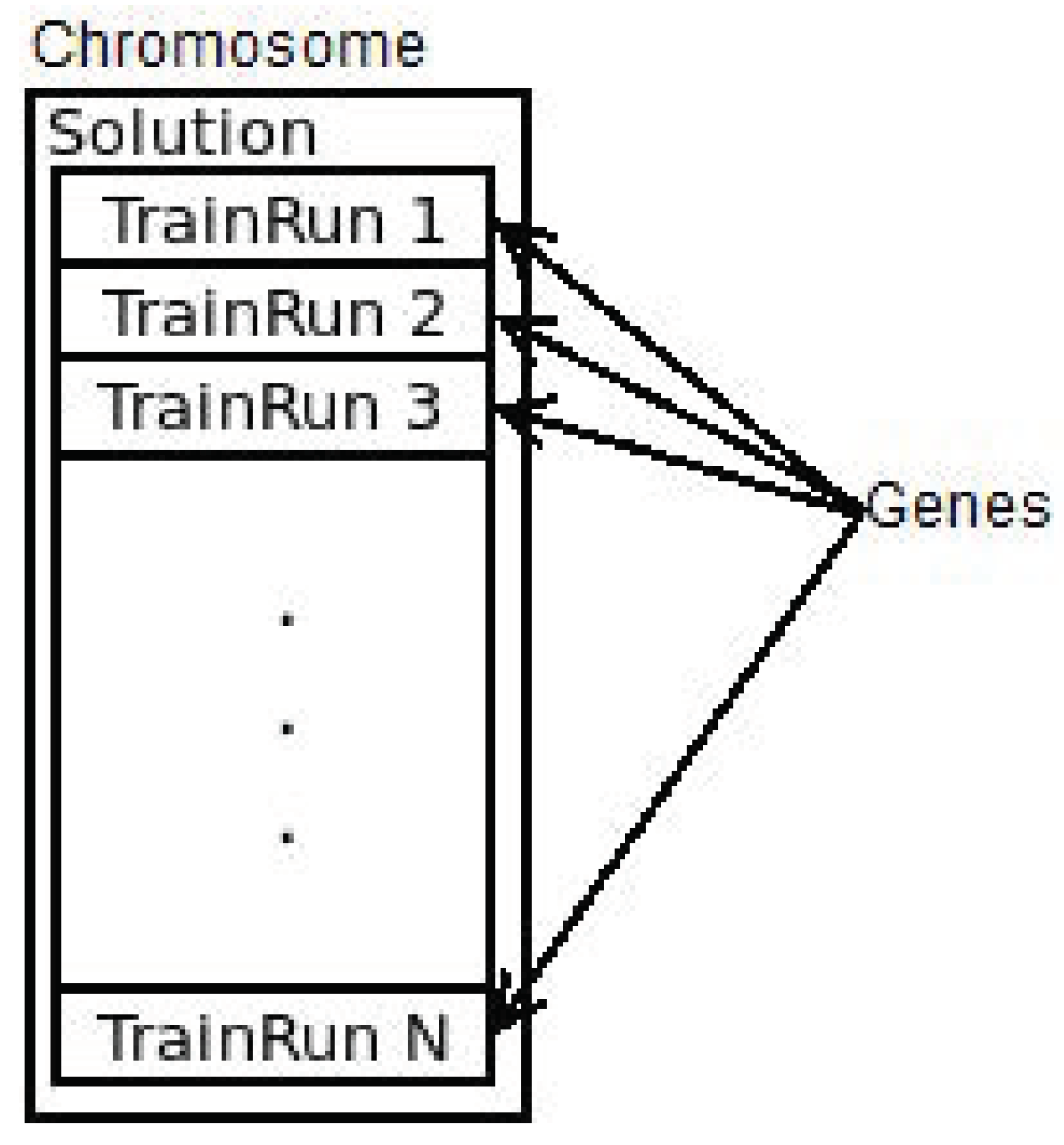
The “Genotype” trait was implemented onto the “Solution” struct, where each train run was considered a gene (see
Figure 9). The individual can be streamed into the sequence of its genes and built from an iterator of the same type. The “is_solution” method of the trait checks that all the service intentions are scheduled and that there are no conflicts on any resource. This is done by issuing a new resource manager and trying to allocate every interval. As soon as one allocation fails, this is interrupted and the function returns false. In this case, allocations are potentially performed in parallel on the base of the service intentions.
A fix function is provided so that resource allocation can be performed again in case the crossover generates collisions. No mutation strategy was provided, so that only the crossover was employed in the research.
The genetic-algorithm framework used for this work, “oxigen”, originally did not provide the possibility to access any data other than the current individual inside the functions that have to compute the fitness value to validate a solution and to fix the individual in order to be valid. The “Genotype” trait was modified in order to provide all relevant methods with a reference to the Problem Instance, where it is possible to cache all information that may be needed to solve problems of a certain complexity. The modified version was published at [
34].
In particular, in this work, it was necessary to have access to the list of resources inside the “fix” and “is_solution” methods in order to build a new ResourceManager.
Genetic algorithms present high-parallelization possibilities because all operations are in fact independent, given that they operate on disjoint individuals. This is an important advantage to consider given the increasing number of threads that modern CPUs can simultaneously handle.
5. Implementation Tools
The heuristic optimization program was developed using the Rust programming language. The “rayon” crate (name used by Rust developers to indicate a published library or program) was used to obtain concurrency based on work stealing, which is a scheduling strategy for computer programs executing dynamically multithreaded computation that can “spawn” new threads of execution on a computer with a fixed number of processors (or cores). It does so efficiently in terms of execution time, memory usage, and interprocessor communication.
The “oxigen” crate provides a framework for genetic algorithms. This was modified and adapted to solve this specific problem, and the modified version has been published. The “oxigen” crate provides one more level of parallelism. In fact, the generation of population individuals and all other operations is concurrently performed on the available threads by using the same work-stealing technique provided by the rayon crate.
The “serde” crate was used to perform efficient serialization and deserialization of json objects into native Rust data structures for input of the problem instances and output of the solutions. It uses the powerful Rust preprocessor to automatically generate serializer and deserializer implementations from and into a wide range of formats. With some attributes, it is possible to guide serde implementations, for example, by changing the name of fields or structures between serialized and deserialized forms.
The “chrono” crate was also used for the correct management of time and “time parse” to provide a parser for the duration in the ISO format. Chrono can manage dates, instants, and durations while also considering time zones. It also provides implementations for mathematical operations between time instants and intervals, so that it was as easy to handle them as it was to manage any other numerical data types. It is also space-optimal and reasonably efficient.
Finally, it was useful to rely on the “rand” crate for pseudorandom number generators and other functions related to randomness, and “petgraph” for a flexible graph-data structure providing the implementation of some basic algorithms and tools to visualize the graph.
All crates are available at [
35], which is the official Rust Package Registry.
6. Performance Evaluation
In this section, results of this work and the comparison with other literature solutions are presented. On the other hand, a study of the sustainability of our proposal is included analyzing how does it work keeping a constant number of train instances and reducing the number of platforms in the stations, being a more sustainable solution.
6.1. Results
The results presented in this section are based on the problem instances provided for the “train-schedule optimization challenge” proposed by SSB on the CrowdAI website [
36].
First, the simplest possible scenarios were proposed as sample files. These were modified to produce simple scenarios with collisions. The draft timetables for these scenarios are reported in
Table 1.
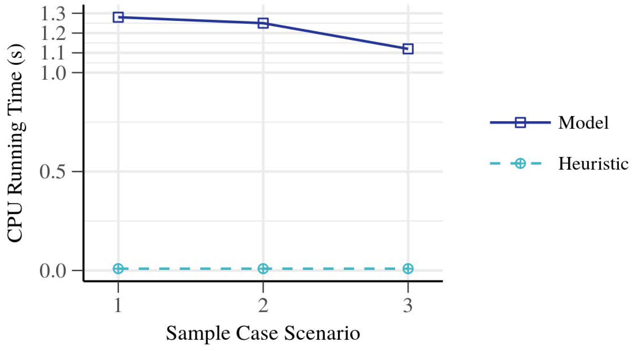
Figure 10 shows the computation times for the mathematical model and the heuristics in these simple scenarios. The first case, without collisions, was solved by the Gurobi solver in
. When adding the collisions in two different formats, the model gave a result in
and
, respectively. In the same situations, the heuristic solver produced an exact solution in
, probably dominated by input, output, and concurrency setup. The optimal solution could be obtained in these cases using only the heuristic algorithm without further genetic optimization (i.e., using a population of only one individual).
The mathematical model could not be applied to more complicated problem instances due to the computation time becoming too high, which is not so useful for real situations.
The rest of the problem instances present examples with increasing levels of difficulty:
- (a)
The easiest is scheduling four trains that do not have conflicts. Minimal routing is possible with some discouraged paths;
- (b)
routing 58 trains with some conflicts and minimal routing alternatives;
- (c)
more difficult, increasing the number of trains to 143 but still keeping a minimal number of alternative paths;
- (d)
increases routing alternatives and features slightly more trains;
- (e)
very similar but with one more train and no optimal solution;
- (f)
Sixth and seventh instances continue to increase the alternatives and add a lot more trains, while the eighth and ninth again reduce the number of trains but increase the number of paths; and
- (g)
it was uncertain whether there was a solution with an objective value of 0.
All instances except for the fifth could be solved optimally.
Table 2 contains a schematic description of all problem instances.
Note that instances 3–9 also contained connections between services, but the logic to handle them was not implemented in this work.
All tests were executed on a personal computer featuring an AMD A10 processor (four cores, one thread per core), with 8 GB RAM and a Solid State Drive. Results for all cases are reported in
Table 3.
The easiest case could be solved with optimality by also using a very small population, for example, two individuals, in only .
The second case featured 58 trains with minimal routing alternatives. The heuristic method could find a feasible solution with an objective value of 2.95, which practically means considering that all delays were weighted at 1, less than a 3 delay among all the section requirements of all service intentions. This solution was found in a running time of by using a population composed of 128 individuals.
The worst case was the seventh problem instance, that is, the one featuring more trains. In this and the sixth case, the heuristic method would have been killed if it were run with a population of more than 32 individuals. In that case, the average delay per service intention was less than 1 on the entire schedule.
Usage of the look-ahead method produced generally worse results, as can be seen in
Table 4. In some cases, it was not able to find a feasible solution.
Computation time primarily depended on population size. The most complex type of problem for this architecture was the one with lots of trains because it tended to substantially increase the memory footprint of the program, which was sometimes killed for this reason.
In order to compare our proposal with other studies, Ref. [
25] was selected because the scenario was quite similar and used similar infrastructure resources to run the algorithms. It was reproduced and optimized using our proposed MILP model and the heuristic method. The only difference was the objective function that was global profit in this case. The comparison with other works had difficulty reproducing the scenarios due to a lack of data.
The study in [
25] was based on an artificial network composed of 15 stations with a total of 90 platforms. They had different requests sets with different requested train journeys (train instances in our nomenclature). Results are shown in
Figure 11, in which we called the solutions of [
25] Train Timetabling Problem-MILP-Arenas (model) and Train Timetabling Problem- Genetic Algorithm-Arenas (heuristic). The
y-axis was transformed into a log scale by using a method that first figured out where the tick marks go on the axis (still on the linear scale) and what the labels should be, and then transformed observations into the log scale. This could be valuable to plot very highly skewed distributions.
Using the solution proposed in this paper, all cases were solved with optimal results, and computation times are contained in
Table 5.
Even for a medium-sized rail network, scheduling requires a large number of train scheduling. Therefore, we were interested in solutions for a large number of train instances.
By analyzing the results, the computation time for solving the proposed MILP was worse than that of TTP-MILP-Arenas for the requests with a low number of trains (fewer than 15 trains). As the number of instances increased, it could be solved faster than [
25] obtaining an exact solution.
The heuristic method was faster than that of TTP-GA-Arenas except for the case with very few trains (fewer than eight trains), and faster than the MILP solver in all test cases.
On the basis of these results, we considered that the performance of our proposal was better than that presented by Arenas et al. in [
25] on real size scenarios.
In this case, it was not easy to compare the profit function of the other studies with the cost function (
6), but the objective value of 0 found in all our solutions comfirmed that they were optimal.
6.2. Sustainability
The term sustainability in this work is defined as the ability to maintain the existing railway infrastructure while the traffic of trains increases. This requires obtaining better scheduling to improve the utilization of the resources.
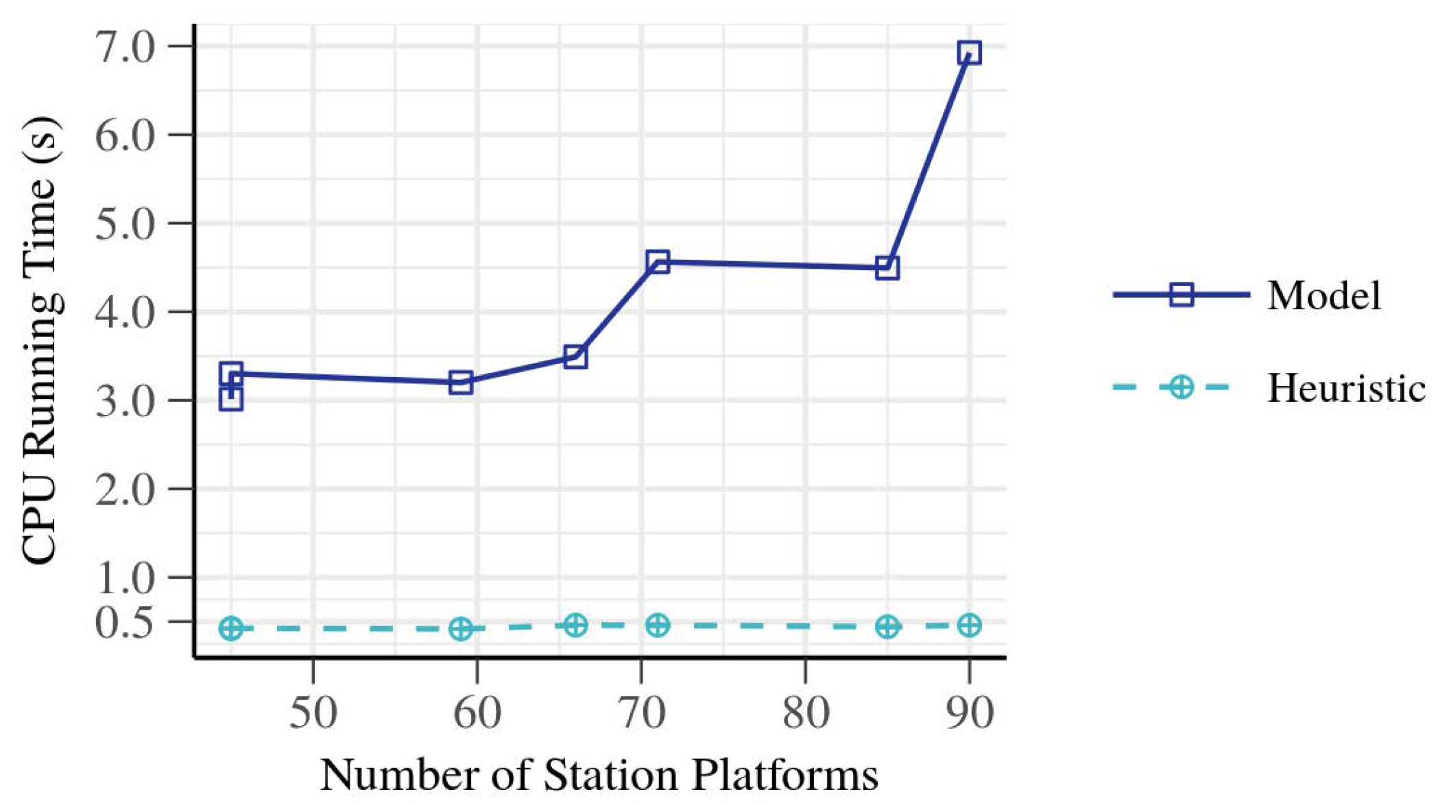
Thus, using the same network, a series of experiments were executed keeping a constant number of train instances and reducing the number of platforms in the stations. The result is that it was possible to halve the number of platforms in the network.
Figure 12 shows how computation time varied with the total number of station platforms in the network. For heuristics, it was constant, while for the MILP solver, a higher number of platforms resulted in increased computation time. In all cases, both the MILP and the heuristic method found the optimal solution.
With the result of
Figure 12, it is concluded that an optimal train scheduling can be obtained for a specific traffic with fewer number of station platforms. Fewer platforms can improve sustainability by reducing the maintenance costs of the stations and infrastructure.
On the other hand, it is deduced that it is possible to increase traffic on the infrastructure without further extensions, sensibly reducing or canceling construction costs in that case.
Moreover, bigger infrastructures, unless underground, tend to divide cities, and this is a social cost for citizens. Being able to reduce infrastructure size, or at least not increase it, can improve this aspect.
7. Conclusions
Rail transport is recognized as an energy-efficient (though capital intensive) and sustainable means of transport. Moreover, each freight train can take a large number of trucks off the roads, making them safer.
Studies in this field can help to make railways more attractive to travelers by reducing the operative cost, and increasing the number of services and their punctuality.
In a world that is threatened by the impact of global warming on a daily basis, we as a society should make every possible move to reduce energy usage, make things more efficient, and use means that can easily switch to renewable sources.
In this work, a complex problem and its mathematical formulation were presented, and its model was run against easy problem instances, due to more complex instances could not be managed by a MILP solver. The proposed heuristic method was based on genetic metaheuristics and could provide feasible solutions in seconds.
The high level of parallelism of the presented solution, obtained with real-time concurrency and optimal task scheduling obtained through the work-stealing technique, could easily be scaled on machines with a higher core count. Moreover, this approach could be extended to wider clusters if the number of services to schedule is higher or a solution needs to be found in nearly real time. Even for a medium-sized rail network, scheduling requires large numbers of train schedulers or planners that take many months to complete, and makes it difficult or impossible to explore alternative schedules, plans, operating rules, and objectives.
Works in this field could reduce the impact of timetabling on the operative costs of railways in a sensible way.
The obtained results showed that heuristic method was able to generate solutions in short computational times. However, results in general were not optimal, although delays in the worst case were less than 1 h per train, cumulative on the whole timetable, on a very packed timetable draft.
A comparison with literature proposals that uses a similar scenario, shows that, for a large number of train requests, our solution obtains the optimal train scheduling faster.
Finally, as a future work, there are several lines of research arising from this work which should be pursued. In one hand, some improvements on the heuristic could be in spite of the promising results presented for our heuristic method. When compared to other proposals and the MILP model, there are still several issues to be addressed that should be seen as future improvements with a particular focus on:
Implementing a mutation strategy to further exploit the solution space around good solutions, for example, by exploring alternative paths or changing some time events in ways that are not explored in the generation of the individuals;
using some data structures that implement a copy-on write mechanism in order to reduce overall memory footprint and the number of program allocations; and
improving the look-ahead method and fine-tuning the value of the threshold to obtain a better initial population.
On the other hand, further research is still necessary to include other parameters related with the environmental impacts of the paths selection of the railway service. Some constraints could be the operation and maintenance costs, the emissions of each type of train or the energy consumption. These new restrictions will help to achieve a train programming table aligned with the sustainability needed in today’s society.


