Computer Modeling for the Operation Optimization of Mula Reservoir, Upper Godavari Basin, India, Using the Jaya Algorithm


 and
and
Abstract
:1. Introduction
2. Materials and Methods
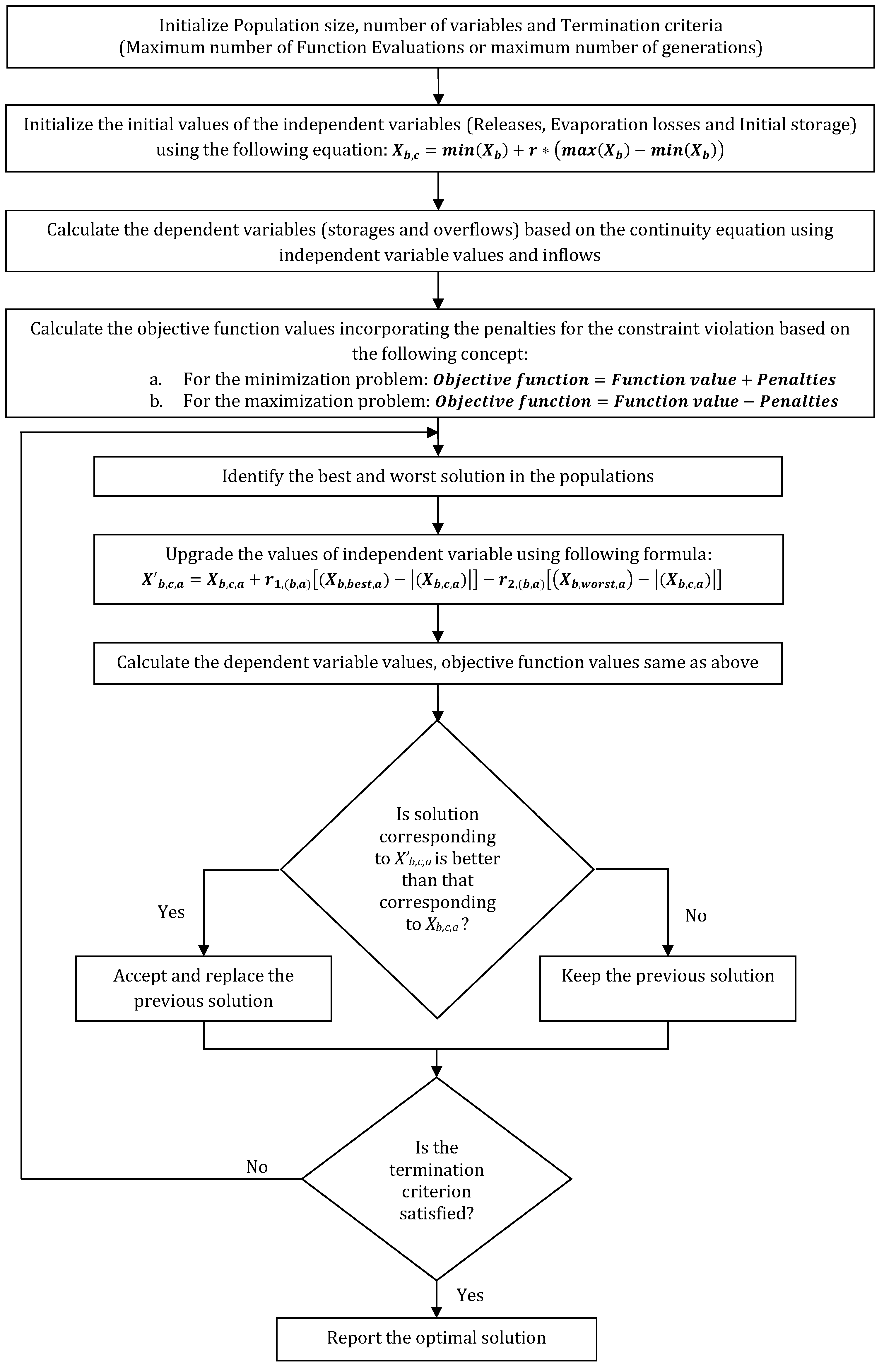
2.1. Description of the Jaya Algorithm
- is the minimum value of the variable ,
- r is a random number (),
- is the maximum value of the variable .
- For the minimization problem: ,
- For the maximization problem: .
- is the updated value of the variable,
- is the old value of the variable,
- and are random variable for the variable during the generation (),
- is the variable corresponding to the best candidate solution for iteration,
- is the variable corresponding to the worst candidate solution for iteration.
2.2. Case Study 1
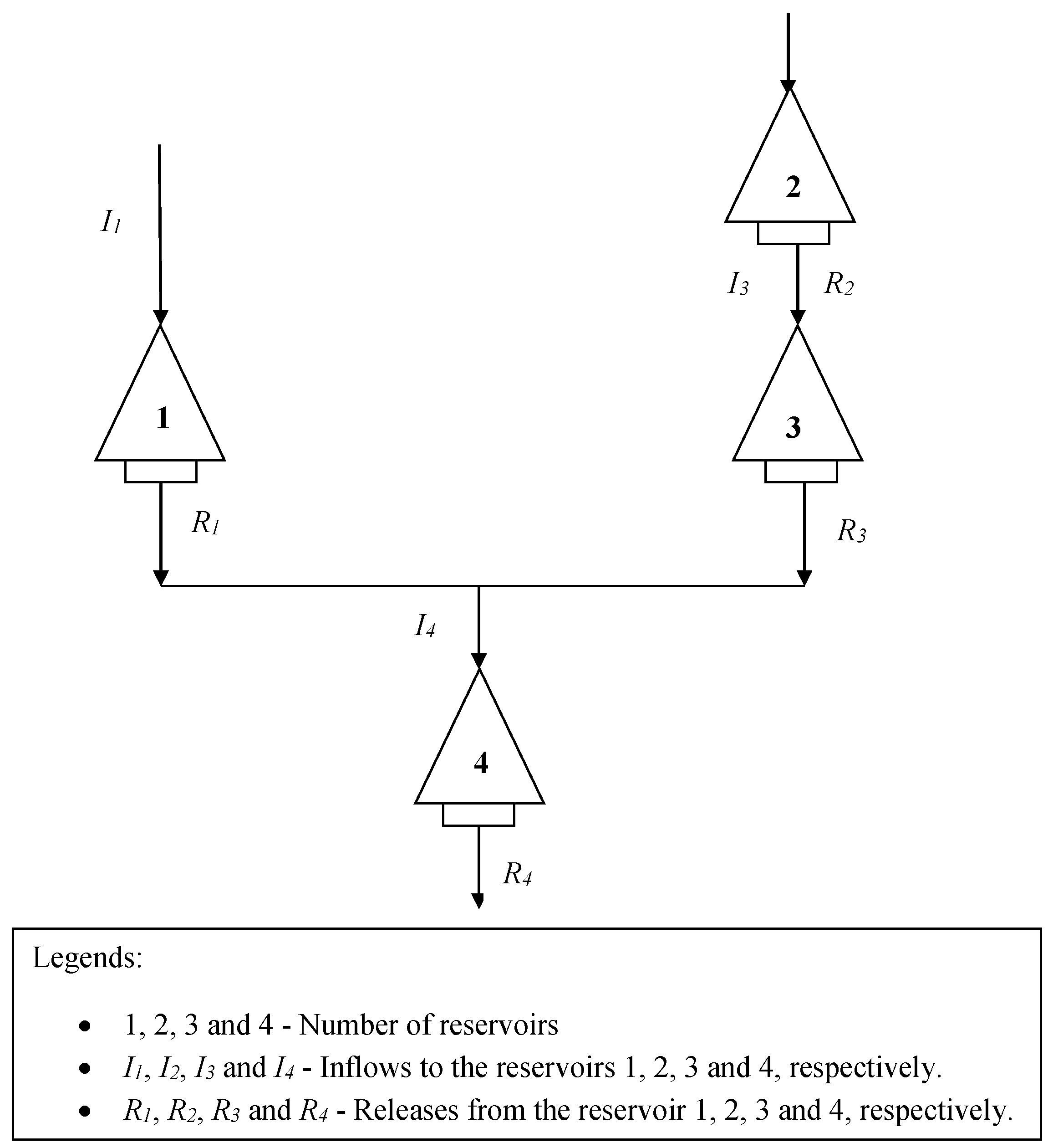
- is a matrix of profit, function associated with all the four reservoirs for hydropower,
- represents the releases from the reservoirs 1 to 4 during the period ‘t’. The benefit function associated with the hydropower is as follows:
- is the benefit associated with the fourth reservoir for irrigation
- describes the releases from the fourth reservoir during the period ‘t’
- is the storage at the beginning of the next time period ‘’ for reservoirs 1 to 4,
- is the storage at the beginning of the time period ‘t’ for reservoirs 1 to 4,
- M is a matrix of indices of the reservoir connections
- is the storage at the beginning of next time period (generally irrigation year) for the reservoir,
- represents the target storage at the beginning of the next time period (generally irrigation year),
- for .
2.3. Case Study 2
Model Formulation
- F is the squared deviation of releases from the target releases,
- t is the time in months (),
- represpents the total releases during period ‘t’ in
- is the Left Bank Canal (LBC) releases during period ‘t’ in ,
- is the Right Bank Canal (RBC) releases during period ‘t’ in ,
- is the industrial and urban releases during period ‘t’ in ,
- is the total demand during period ‘t’ in .
- is the storage of the reservoir at the beginning of time period ‘’ in ,
- is the storage of the reservoir at the beginning of time period ‘t’ in ,
- is the inflow into the reservoir during period ‘t’ in ,
- is the reservoir lift (if any) during period ‘t’ in ,
- is the evaporation loss from the reservoir during period ‘t’ in ,
- is the overflow from the reservoir during the period ‘t’ in .
- is the dead pool storage of the reservoir in ,
- is the reservoir capacity in .
- is the maximum canal carrying capacity for LBC in ,
- is the maximum canal carrying capacity for RBC in .
- and ,
- is the release from supply ‘x’ for time period ‘t’ in ,
- is the demand for the supply for the time period ‘t’ in .
- is the storage at the end of irrigation year,
- is the storage at the beginning of the irrigation year.
3. Results
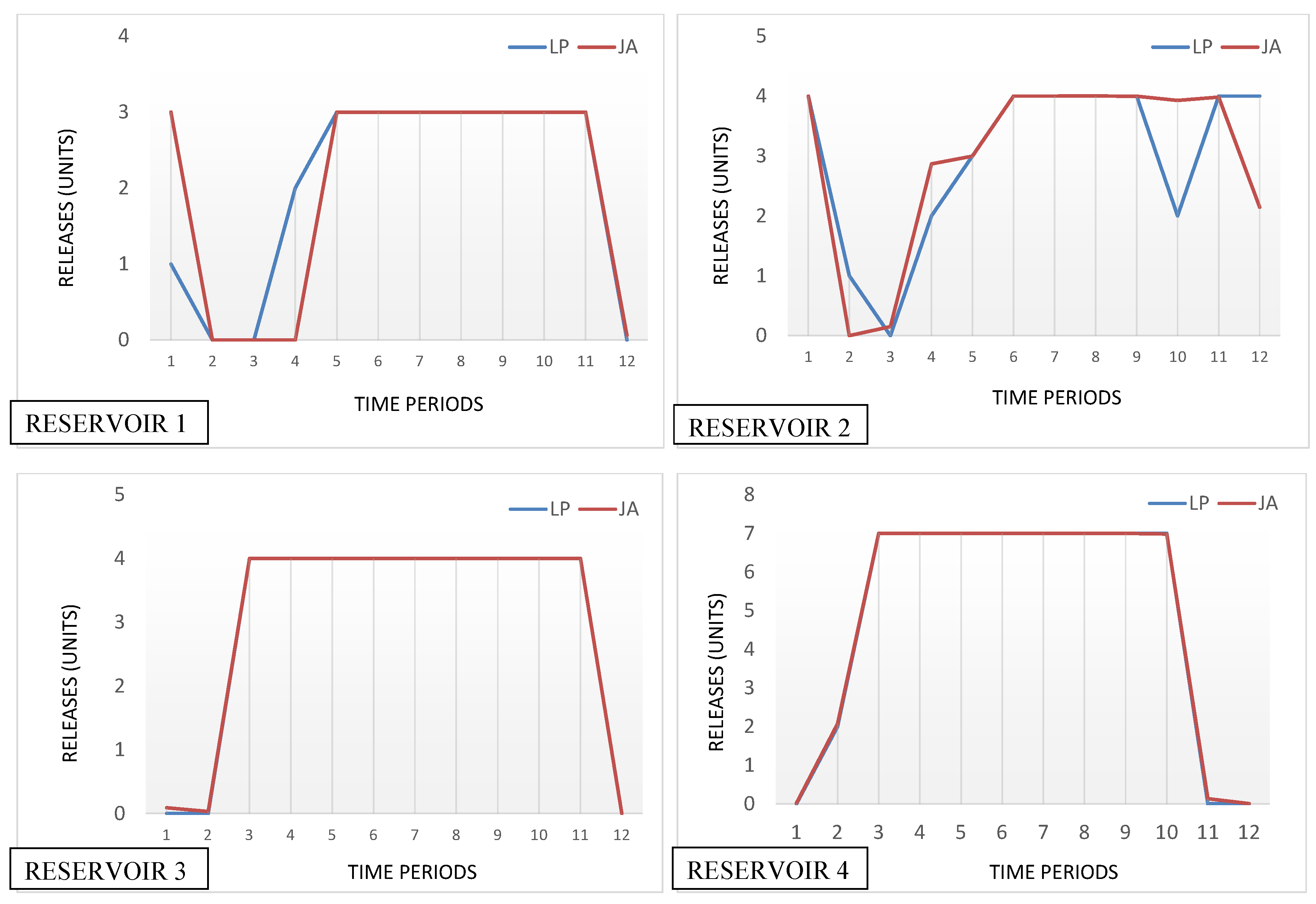
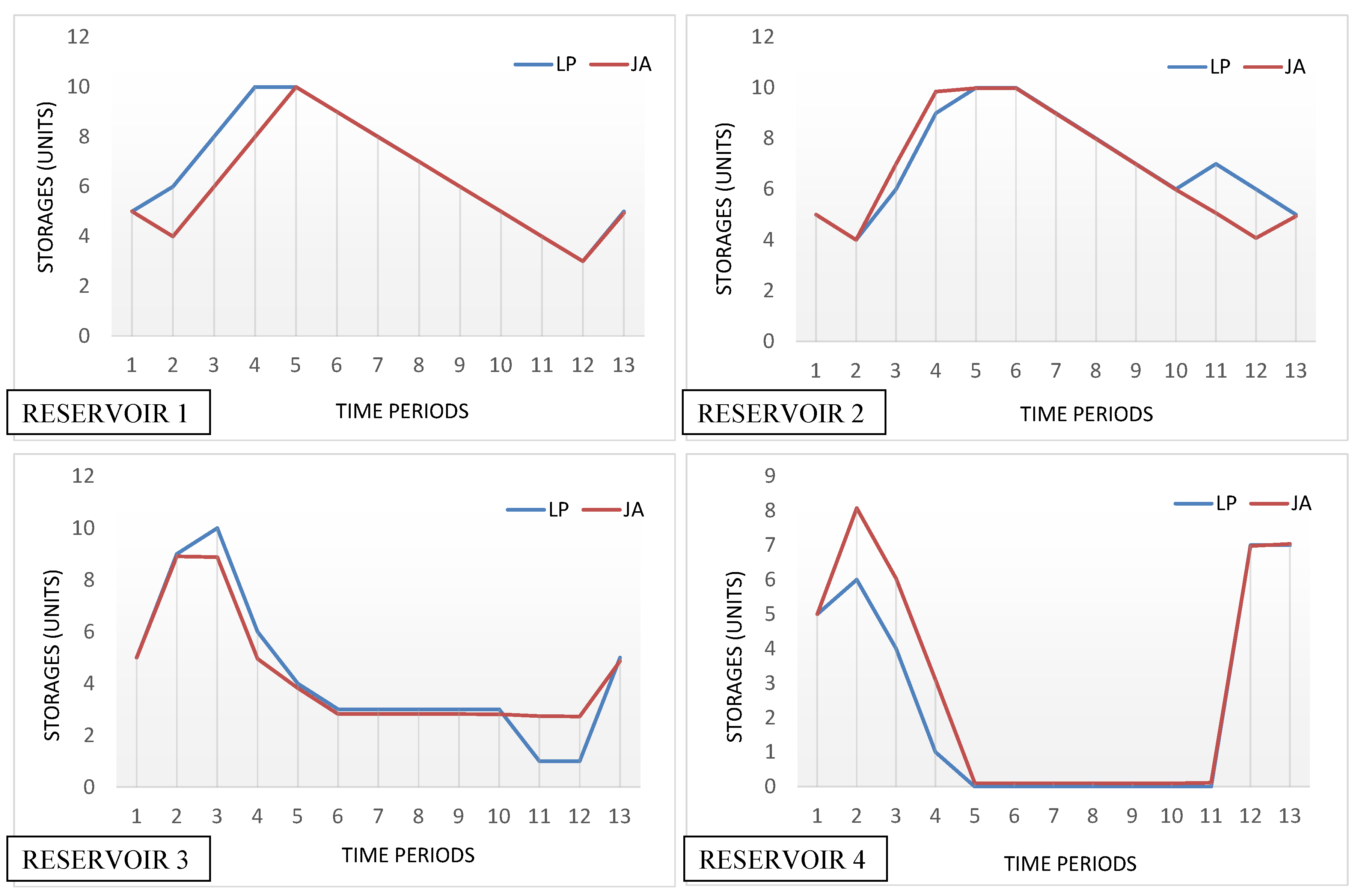
3.1. Hypothetical Four Reservoir System
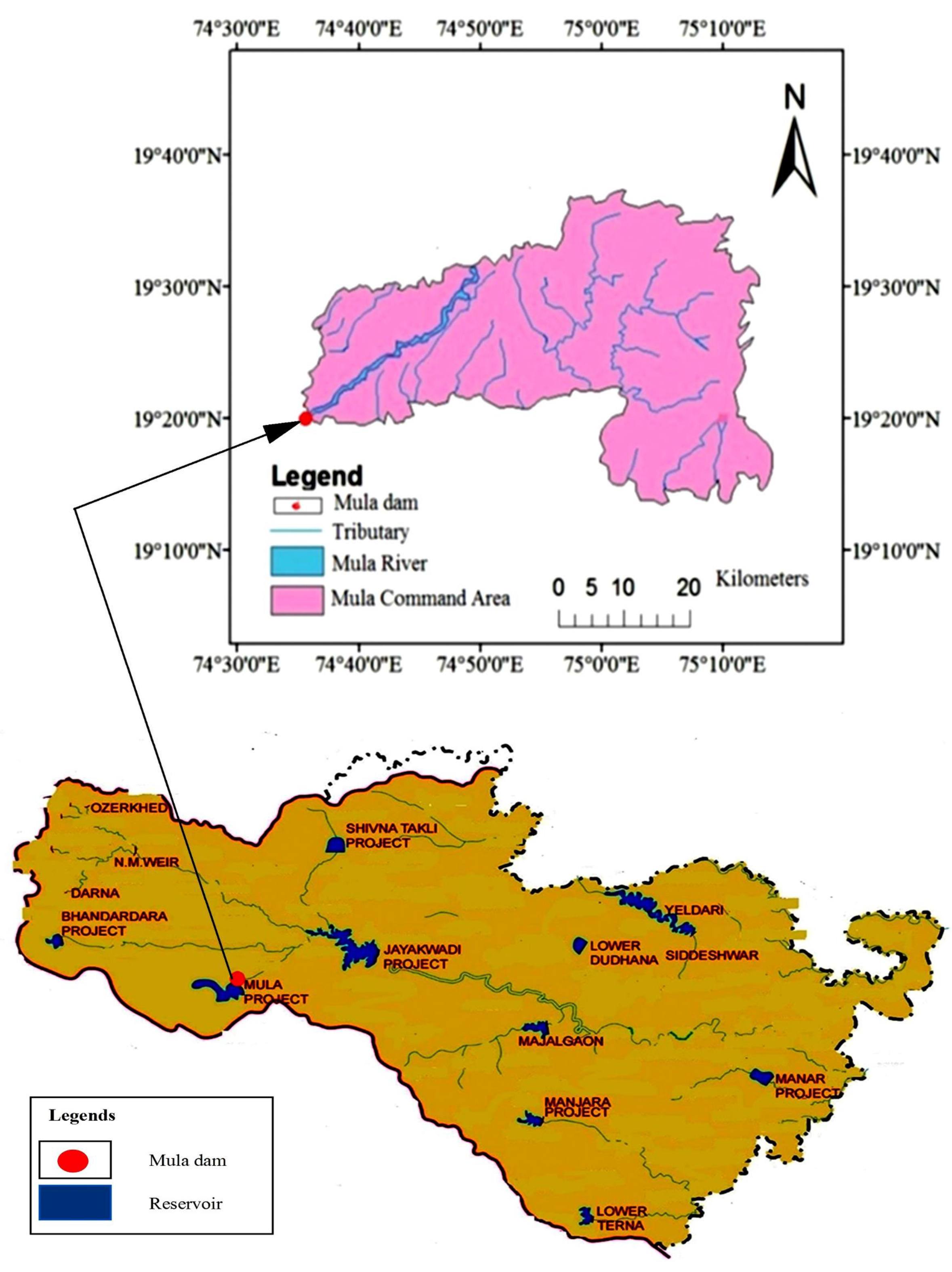
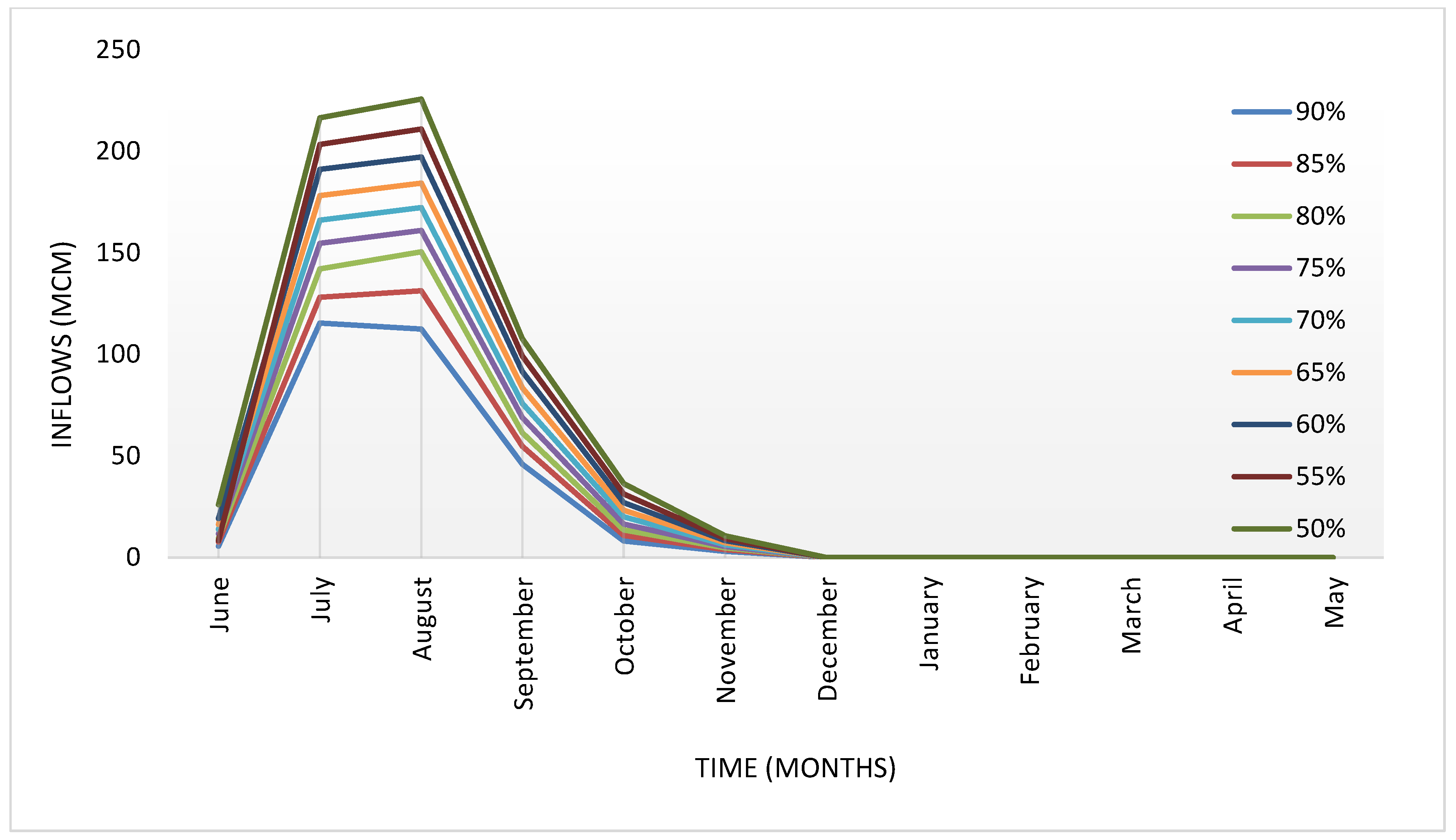
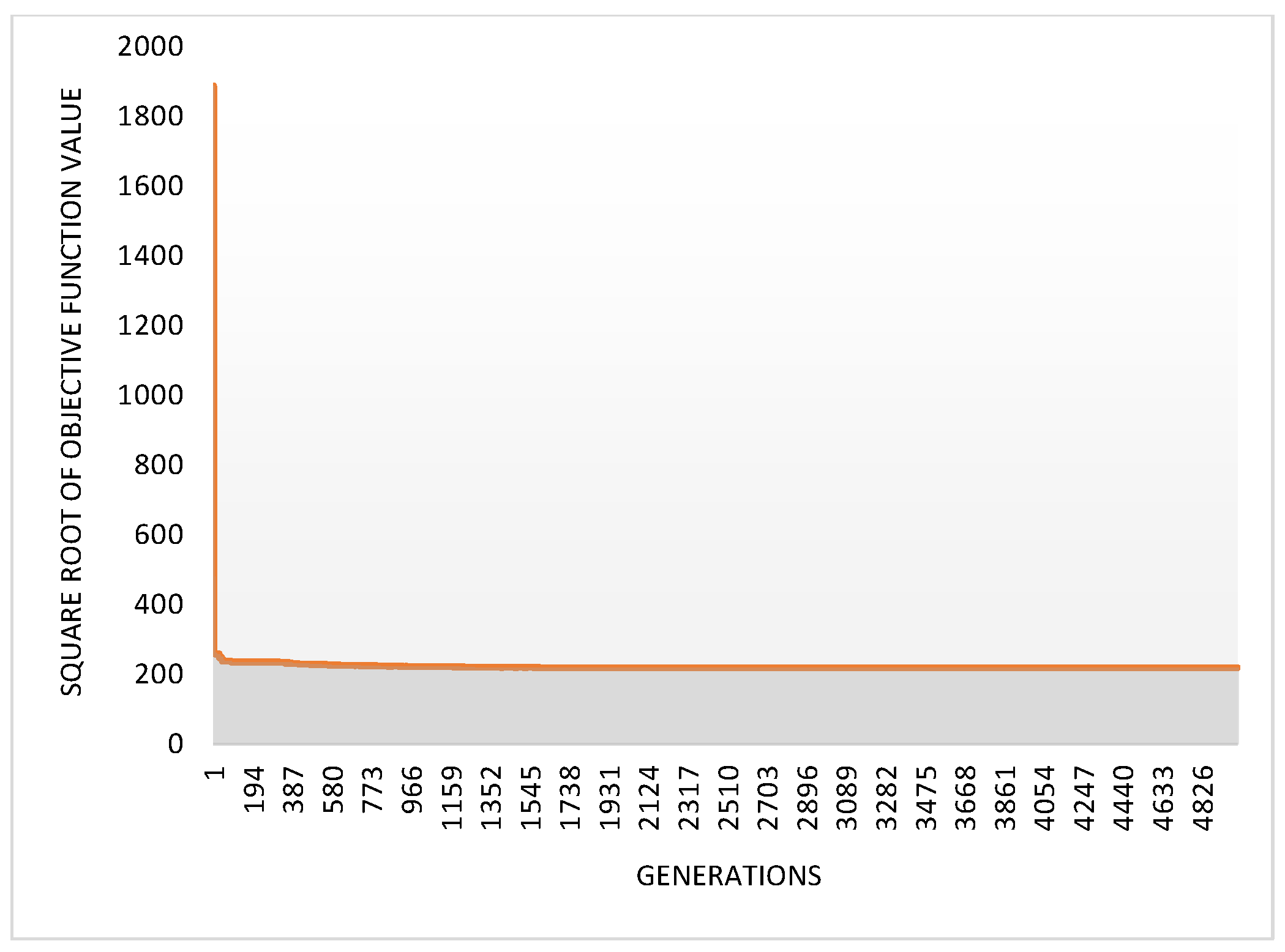
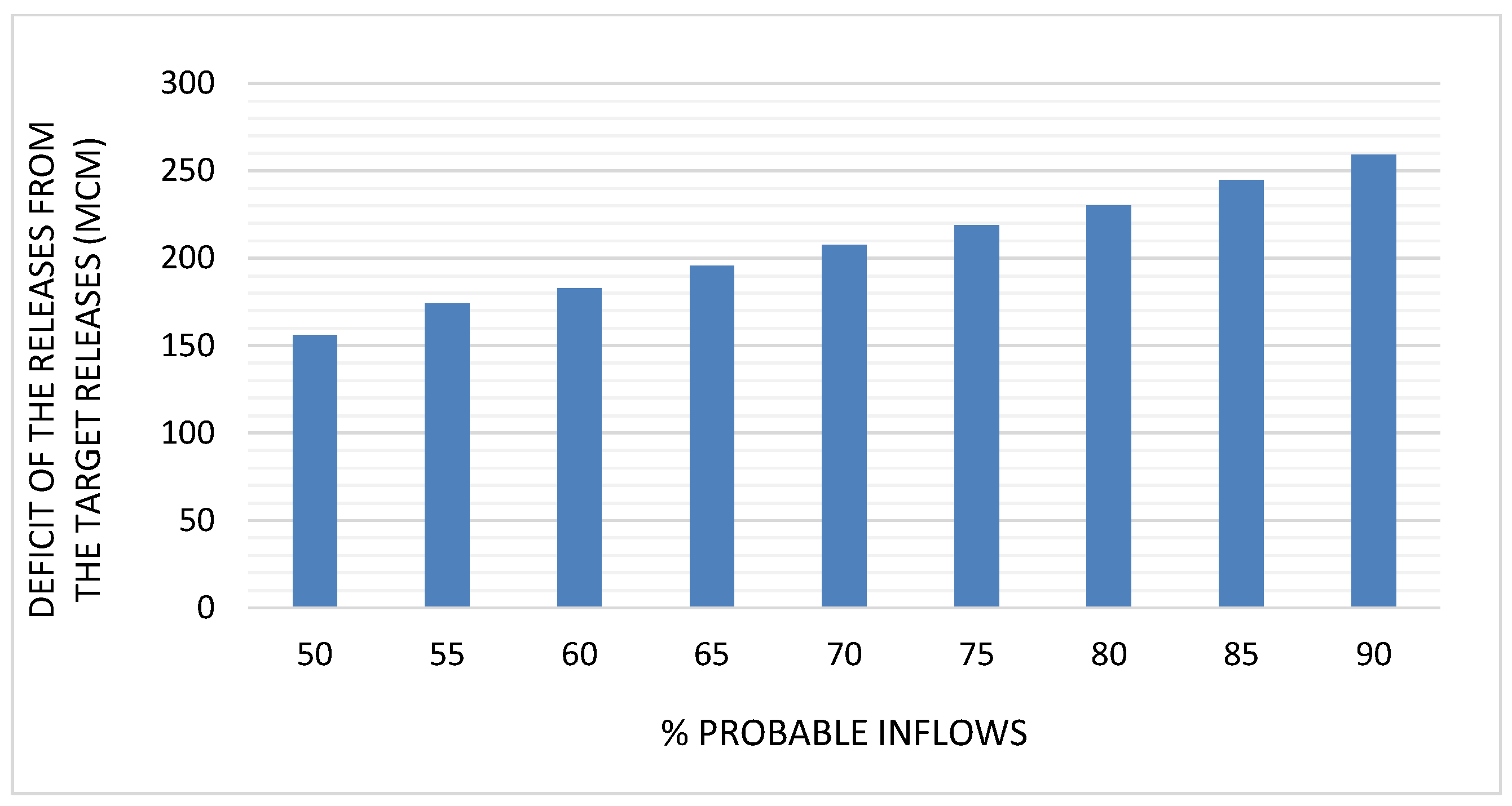
3.2. Mula Reservoir
4. Conclusions
Author Contributions
Funding
Acknowledgments
Conflicts of Interest
Abbreviations
| ACO | Ant Colony Optimization |
| AFSA | Artificial Fish Swarm Algorithm |
| AI | Artificial Intelligence |
| CA | Crow Algorithm |
| CADA | Command Area Development Authority |
| CSSA | Charged System Search Algorithm |
| DDDP | Discrete Differential Dynamic Programming |
| DDP | Differential Dynamic Programming |
| DE | Differential Evolution |
| DP | Dynamic Programming |
| DPSA | Dynamic Programming with Successive Approximation |
| EA | Evolutionary Algorithm |
| EMPSO | Elitist Mutated Particle Swarm Optimization |
| FA | Firefly Algorithm |
| FDP | Folded Dynamic Programming |
| FEs | Function Evaluations |
| GA | Genetic Algorithm |
| GEA | Gradient Evolution Algorithm |
| HA | Hybrid Algorithm |
| HS | Harmony Search |
| HBMO | Honey Bee Mating Optimization |
| JA | Jaya Algorithm |
| Kh. | Kharif |
| Kh. Hy. | Kharif Hybrid |
| LBC | Left Bank Canal |
| LINGO | Language for Interactive General Optimization |
| LP | Linear Programming |
| MATLAB | Matrix Laboratory |
| MAX | Maximization |
| MCM | Million Cubic Metre |
| MHLLBC | Mula High Level Left Bank Canal |
| MHLRBC | Mula High Level Right Bank Canal |
| MIN | Minimization |
| MLBC | Mula Left Bank Canal |
| MRBC | Mula Right Bank Canal |
| NIR | Net Irrigation Requirement |
| NLP | Non-Linear Programming |
| PBC | Pathardi Branch Canal |
| PSO | Particle Swarm Optimization |
| Rb. | Rabi |
| Rb. Hy. | Rabi Hybrid |
| RBC | Right Bank Canal |
| SA | Shark Algorithm |
| TLBO | Teaching Learning Based Optimization |
| WCA | Water Cycle Algorithm |
| WOA | Weed Optimization Algorithm |
| WSA | Wolf Search Algorithm |
References
- Tian, J.; Guo, S.; Liu, D.; Pan, Z.; Hong, X. A Fair Approach for Multi-Objective Water Resources Allocation. Water Resour. Manag. 2019, 33, 3633–3653. [Google Scholar] [CrossRef]
- Ahmad, A.; El-Shafie, A.; Razali, S.F.M.; Mohamad, Z.S. Reservoir optimization in water resources: A review. Water Resour. Manag. 2014, 28, 3391–3405. [Google Scholar] [CrossRef]
- Sreenivasan, K.; Vedula, S. Reservoir operation for hydropower optimization: A chance-constrained approach. Sadhana 1996, 21, 503–510. [Google Scholar] [CrossRef] [Green Version]
- Arunkumar, R.; Jothiprakash, V. Optimal reservoir operation for hydropower generation using nonlinear programming model. J. Inst. Eng. India Ser. A 2012, 93, 111–120. [Google Scholar] [CrossRef]
- Mousavi, S.; Ponnambalam, K.; Karray, F. Reservoir operation using a dynamic programming fuzzy rule—Based approach. Water Resour. Manag. 2005, 19, 655–672. [Google Scholar] [CrossRef]
- Jalali, M.; Afshar, A.; Marino, M. Reservoir operation by ant colony optimization algorithms. Iran. J. Sci. Technol. Trans. B Eng. 2006, 30, 107–117. [Google Scholar]
- Bozorg-Haddad, O.; Karimirad, I.; Seifollahi-Aghmiuni, S.; Loáiciga, H.A. Development and application of the bat algorithm for optimizing the operation of reservoir systems. J. Water Resour. Plan. Manag. 2014, 141, 04014097. [Google Scholar] [CrossRef]
- Haddad, O.B.; Hosseini-Moghari, S.M.; Loáiciga, H.A. Biogeography-based optimization algorithm for optimal operation of reservoir systems. J. Water Resour. Plan. Manag. 2015, 142, 04015034. [Google Scholar] [CrossRef]
- Asadieh, B.; Afshar, A. Optimization of Water-Supply and Hydropower Reservoir Operation Using the Charged System Search Algorithm. Hydrology 2019, 6, 5. [Google Scholar] [CrossRef] [Green Version]
- Ehteram, M.; Binti Koting, S.; Afan, H.A.; Mohd, N.S.; Malek, M.A.; Ahmed, A.N.; El-shafie, A.H.; Onn, C.C.; Lai, S.H.; El-Shafie, A. New evolutionary algorithm for optimizing hydropower generation considering multireservoir systems. Appl. Sci. 2019, 9, 2280. [Google Scholar] [CrossRef] [Green Version]
- Vasan, A.; Raju, K.S. Optimal reservoir operation using differential evolution. In Proceedings of the International Conference on Hydraulic Engineering: Research and Practice (ICON-HERP), Roorkee, India, 26–28 October 2004. [Google Scholar]
- Garousi-Nejad, I.; Bozorg-Haddad, O.; Loáiciga, H.A.; Mariño, M.A. Application of the firefly algorithm to optimal operation of reservoirs with the purpose of irrigation supply and hydropower production. J. Irrig. Drain. Eng. 2016, 142, 04016041. [Google Scholar] [CrossRef] [Green Version]
- Jothiprakash, V.; Shanthi, G. Single reservoir operating policies using genetic algorithm. Water Resour. Manag. 2006, 20, 917–929. [Google Scholar] [CrossRef]
- Samadi-koucheksaraee, A.; Ahmadianfar, I.; Bozorg-Haddad, O.; Asghari-pari, S.A. Gradient Evolution Optimization Algorithm to Optimize Reservoir Operation Systems. Water Resour. Manag. 2019, 33, 603–625. [Google Scholar] [CrossRef]
- Bashiri-Atrabi, H.; Qaderi, K.; Rheinheimer, D.E.; Sharifi, E. Application of harmony search algorithm to reservoir operation optimization. Water Resour. Manag. 2015, 29, 5729–5748. [Google Scholar] [CrossRef]
- Afshar, A.; Haddad, O.B.; Mariño, M.A.; Adams, B.J. Honey-bee mating optimization (HBMO) algorithm for optimal reservoir operation. J. Frankl. Inst. 2007, 344, 452–462. [Google Scholar] [CrossRef]
- Yaseen, Z.M.; Karami, H.; Ehteram, M.; Mohd, N.S.; Mousavi, S.F.; Hin, L.S.; Kisi, O.; Farzin, S.; Kim, S.; El-Shafie, A. Optimization of reservoir operation using new hybrid algorithm. KSCE J. Civ. Eng. 2018, 22, 4668–4680. [Google Scholar] [CrossRef]
- Paliwal, V.; Ghare, A.D.; Mirajkar, A.B. Single-Reservoir operation optimization using Jaya Algorithm for Jayakwadi-1 dam, India. In Proceedings of the E-proceedings of the IAHR World Congress, Kuala Lumpur, Malaysia, 13–18 August 2017; pp. 1–8. [Google Scholar]
- Nagesh Kumar, D.; Janga Reddy, M. Multipurpose reservoir operation using particle swarm optimization. J. Water Resour. Plan. Manag. 2007, 133, 192–201. [Google Scholar] [CrossRef]
- Ehteram, M.; Allawi, M.F.; Karami, H.; Mousavi, S.F.; Emami, M.; Ahmed, E.S.; Farzin, S. Optimization of chain-reservoirs’ operation with a new approach in artificial intelligence. Water Resour. Manag. 2017, 31, 2085–2104. [Google Scholar] [CrossRef]
- Kumar, V.; Yadav, S. Optimization of reservoir operation with a new approach in evolutionary computation using TLBO algorithm and Jaya algorithm. Water Resour. Manag. 2018, 32, 4375–4391. [Google Scholar] [CrossRef]
- Haddad, O.B.; Moravej, M.; Loáiciga, H.A. Application of the water cycle algorithm to the optimal operation of reservoir systems. J. Irrig. Drain. Eng. 2014, 141, 04014064. [Google Scholar] [CrossRef]
- Asgari, H.R.; Bozorg Haddad, O.; Pazoki, M.; Loáiciga, H.A. Weed optimization algorithm for optimal reservoir operation. J. Irrig. Drain. Eng. 2015, 142, 04015055. [Google Scholar] [CrossRef]
- Ahmadebrahimpour, E. Optimal operation of reservoir systems using the Wolf Search Algorithm (WSA). Water Supply 2019, 19, 1396–1404. [Google Scholar] [CrossRef]
- Labadie, J.W. Optimal operation of multireservoir systems: State-of-the-art review. J. Water Resour. Plan. Manag. 2004, 130, 93–111. [Google Scholar] [CrossRef]
- Hossain, M.S.; El-Shafie, A. Intelligent systems in optimizing reservoir operation policy: A review. Water Resour. Manag. 2013, 27, 3387–3407. [Google Scholar] [CrossRef]
- Rao, R.V.; Patel, V. An improved teaching-learning-based optimization algorithm for solving unconstrained optimization problems. Sci. Iran. 2013, 20, 710–720. [Google Scholar] [CrossRef] [Green Version]
- Rao, R. Jaya: A simple and new optimization algorithm for solving constrained and unconstrained optimization problems. Int. J. Ind. Eng. Comput. 2016, 7, 19–34. [Google Scholar]
- Das, S.R.; Mishra, D.; Rout, M. A hybridized ELM-Jaya forecasting model for currency exchange prediction. J. King Saud Univ. Comput. Inf. Sci. 2017. [Google Scholar] [CrossRef]
- Rao, R.V.; Savsani, V.J.; Vakharia, D. Teaching–learning-based optimization: A novel method for constrained mechanical design optimization problems. Comput.-Aided Des. 2011, 43, 303–315. [Google Scholar] [CrossRef]
- Degertekin, S.; Lamberti, L.; Ugur, I. Sizing, layout and topology design optimization of truss structures using the Jaya algorithm. Appl. Soft Comput. 2018, 70, 903–928. [Google Scholar] [CrossRef]
- Zhang, Y.; Yang, X.; Cattani, C.; Rao, R.; Wang, S.; Phillips, P. Tea category identification using a novel fractional Fourier entropy and Jaya algorithm. Entropy 2016, 18, 77. [Google Scholar] [CrossRef] [Green Version]
- Rao, R.V.; Waghmare, G. A new optimization algorithm for solving complex constrained design optimization problems. Eng. Optim. 2017, 49, 60–83. [Google Scholar] [CrossRef]
- Rao, R.V.; Saroj, A. Economic optimization of shell-and-tube heat exchanger using Jaya algorithm with maintenance consideration. Appl. Therm. Eng. 2017, 116, 473–487. [Google Scholar] [CrossRef]
- Nayak, D.R.; Dash, R.; Majhi, B. Development of pathological brain detection system using Jaya optimized improved extreme learning machine and orthogonal ripplet-II transform. Multimed. Tools Appl. 2018, 77, 22705–22733. [Google Scholar] [CrossRef]
- Varade, S.; Patel, J.N. Determination of Optimum Cropping Pattern Using Advanced Optimization Algorithms. J. Hydrol. Eng. 2018, 23, 05018010. [Google Scholar] [CrossRef]
- Ahmadianfar, I.; Samadi-Koucheksaraee, A.; Bozorg-Haddad, O. Extracting optimal policies of hydropower multi-reservoir systems utilizing enhanced differential evolution algorithm. Water Resour. Manag. 2017, 31, 4375–4397. [Google Scholar] [CrossRef]
- Jain, S.K. Introduction to Reservoir Operation; Technical Report; National Institute of Hydrology: Roorkee, India, 2019. [Google Scholar]
- Larson, R.E. State Increment Dynamic Programming; American Elsevier Publishing: New York, NY, USA, 1968. [Google Scholar]
- Jaya-Algorithm. Available online: https://sites.google.com/site/jayaalgorithm/home. (accessed on 23 July 2019).
- Heidari, M.; Chow, V.T.; Kokotović, P.V.; Meredith, D.D. Discrete differential dynamic programing approach to water resources systems optimization. Water Resour. Res. 1971, 7, 273–282. [Google Scholar] [CrossRef]
- Command Area Development Authority (CADA). Mula Reservoir Project Mula Project 5th Revised Project Volume 1; Technical Report; Godavari Marathwada Irrigation Development Corporation: Aurangabad, India, 1999.
- Kumar, D.N.; Baliarsingh, F. Folded dynamic programming for optimal operation of multireservoir system. Water Resour. Manag. 2003, 17, 337–353. [Google Scholar] [CrossRef]
- Agenis, M.; Bokde, N. GuessCompx: Empirically Estimates Algorithm Complexity; R package version 1.0.3. 2019. Available online: https://CRAN.R-project.org/package=GuessCompx (accessed on 20 December 2019).
- Agenis-Nevers, M.; Bokde, N.D.; Yaseen, Z.M.; Shende, M. GuessCompx: An empirical complexity estimation in R. arXiv 2019, arXiv:1911.01420. [Google Scholar]


| Source | Model | Best Objective Function Value | Population Size | Function Evaluations Taken |
|---|---|---|---|---|
| [39] | DPSA | 401.30 | N.A. | N.A. |
| [41] | DDDP | 401.30 | N.A. | N.A. |
| [43] | FDP | 399.06 | N.A. | N.A. |
| [19] | GA | 401.30 | 500 | 2,279,500 |
| PSO | 399.70 | 500 | 748,000 | |
| EMPSO | 401.30 | 500 | 325,400 | |
| [23] | WOA | 401.30 | 40 | 400,000 |
| Present Study | LP | 401.30 | N.A. | N.A. |
| JA | 401.40 | 150 | 325,000 |
© 2019 by the authors. Licensee MDPI, Basel, Switzerland. This article is an open access article distributed under the terms and conditions of the Creative Commons Attribution (CC BY) license (http://creativecommons.org/licenses/by/4.0/).
Share and Cite
Paliwal, V.; Ghare, A.D.; Mirajkar, A.B.; Bokde, N.D.; Feijóo Lorenzo, A.E. Computer Modeling for the Operation Optimization of Mula Reservoir, Upper Godavari Basin, India, Using the Jaya Algorithm. Sustainability 2020, 12, 84. https://0-doi-org.brum.beds.ac.uk/10.3390/su12010084
Paliwal V, Ghare AD, Mirajkar AB, Bokde ND, Feijóo Lorenzo AE. Computer Modeling for the Operation Optimization of Mula Reservoir, Upper Godavari Basin, India, Using the Jaya Algorithm. Sustainability. 2020; 12(1):84. https://0-doi-org.brum.beds.ac.uk/10.3390/su12010084
Chicago/Turabian StylePaliwal, Vartika, Aniruddha D. Ghare, Ashwini B. Mirajkar, Neeraj Dhanraj Bokde, and Andrés Elías Feijóo Lorenzo. 2020. "Computer Modeling for the Operation Optimization of Mula Reservoir, Upper Godavari Basin, India, Using the Jaya Algorithm" Sustainability 12, no. 1: 84. https://0-doi-org.brum.beds.ac.uk/10.3390/su12010084