A Highly Reliable Propulsion System with Onboard Uninterruptible Power Supply for Train Application: Topology and Control

Abstract

Providing uninterrupted electricity service aboard the urban trains is of vital importance not only for reliable signaling and accurate traffic management but also for ensuring the safety of passengers and supplying emergency equipment such as lighting and signage systems. Hence, to alleviate power shortages caused by power transmission failures while the uninterruptible power supplies installed in the railway stations are not available, this paper suggests an innovative traction drive topology which is equipped by an onboard hybrid energy storage system for railway vehicles. Besides, to limit currents magnitudes and voltages variations of the feeder during train acceleration and to recuperate braking energy during train deceleration, an energy management strategy is presented. Moreover, a new optimal model predictive method is developed to control the currents of converters and storages as well as the speeds of the two open-end-windings permanent-magnet-synchronous-machines in the intended modular drive, under their constraints. Although to improve control dynamic performance, the control laws are designed as a set of piecewise affine functions from the control signals based on an offline procedure, the controller can still withstand real-time non-measurable disturbances. The effectiveness of proposed multifunctional propulsion topology and the feasibility of the designed controller are demonstrated by simulation and experimental results.

1. Introduction

The sustainable development of urban public transport has been considered as an important necessity for achieving environmental protection, viable economy, and social equity goals [1]. Today, electric trains and trams (ETs) are well known as a practical solution to meet these identified demands.

To realize more eco-friendly railway systems and to improve the fuel economy account, there has been a global trend towards introducing renewable energy into railway power systems [2]. Although the electricity generated from these sustainable resources is the most reliable and clean energy carrier, the availability of natural-energy based power from wind and solar is usually intermittent, due to the variable nature of climate conditions and solar radiation. At present, energy storages (ESs) have been considered as a solution for matching the fluctuating power of these natural resources to the changing demand of the railway tractions [2]. Besides, these facilities can be advantageous to make maximum use of such energy sources by storing the regenerative braking energy of the ETs into the ESs, for the sake of power peak shaving. Therefore, as the ESs contribute significantly to reduce the peak power demand and improve energy efficiency, their application is closely associated with both financial and environmental sustainability goals [3].

On the other hand, the sustainable railway development depends on proper reliability for its power supply system. This is because any failure in this system not only can affect the operation of trains and the railway infrastructure [4] but also may have a wider adverse impact on other sectors such as supportability, health, and politics [5]. The reliability of railway power supplies may suffer from different forms of power disturbances, such as blackouts and outages, overvoltages, and brownouts, as well as frequency variations and voltages harmonics [6]. An effective way for the ETs feeding systems to improve their power availability and to achieve higher levels of resilience is the option of adding redundant energy sources with fault-tolerant parallel and distributed architectures [7]. Thus, to avoid trains service disruptions during main power disturbances or wayside subsystem isolations, onboard auxiliary power supply (APS) is one of the key equipment for the railway trains [8]. Besides, the onboard ES facilities can be combined with or individually serve as multi-beneficial APS, to provide continuous and adequate electrical power to the train tractions in different operation conditions. Therefore, in addition to their great impact on the system reliability of the train power supplies, the APSs could also have a positive impact on the sustainability of railway services.

As a result, for the sustainable and efficient transport development, employing both ESs and APSs on board the railway vehicles, is now essential to keep the ETs moving safely, promptly and efficiently (The list of all acronyms used in the text is presented in Appendix A).

1.1. Onboard Energy Storages

Many modern railway systems are equipped with bidirectional substations that have the ability to capture the recuperated braking energy from a decelerated train through the third rail or overhead catenary [9]. Then, instead of dissipating it in the vehicle brake resistors, the recovered energy can be fed back into the other nearby accelerating trains or can be stored in the stationary energy storage (ESs) for the later use. Besides, if a fault occurs in the supply network, those substations which are facilitated by the ESs, can serve as uninterruptible power supplies (UPS) to provide the required power for ETs tractions, ensuring zero downtime for the railway systems. Apart from such wayside UPS systems, most railway power substations are also protected by redundant resources, such as independent backup diesel generators. However, when an unexpected fault occurs in the third rail or overhead line installations (for instance: The breakage of an insulator, a catenary wire, or a contact cable), the availability of those emergency power supplies will be severely limited and might not be feasible for a period of time. Therefore, equipping railway vehicles with onboard ESs seems to be a more reliable solution, since it offers more energy-saving potential and the important advantage of being more fault-tolerant. Most importantly, during failures in the power system lines or a blackout, the energy stored in the onboard ESs can make it possible to move the ETs to the nearest railway station for evacuating passengers from the stalled vehicle, especially when it sticks in a tunnel, without the need of external power supply.

This technical solution, which can be considered as an auxiliary UPS aboard the ETs, is also applicable to either the older electric railway systems which still have unidirectional diode-bridge rectifier substation or the other railway systems with diesel-electric multiple unit (DEMU) tractions. In the older substation, the peak and inrush currents from the supply system will be considerably limited (to almost 50 percent of the line current, as reported in [10]) by managing the charge and discharge process of the ESs, during acceleration, coasting, and braking of the train. Then, the released power capacity can cause a significant increase in the reliability of the transmission lines, and it might assist in the infrastructure development, for instance: increasing the length of existing trains, or reducing the time interval between the trains on the existing routes. Adding the ESs to the DEMU tractions, in addition to increasing overall reliability, can cause the diesel power to be reduced significantly, thereby reducing energy consumption and emissions [11]. Besides, the onboard UPS makes it possible to turn the diesel engine off temporarily, for example, at the stations and the tunnels, which makes the DEMU tractions more flexible and allows them to be used in the new applications. Equipping a train with such auxiliary UPSs will require some space on the roof or floor [8] and increase the weight by about 2% [10]. Nevertheless, instead of stationary ESs, which are centralized in the substation, onboard ESs are distributed among the trains, thus reducing the space and cost allocation in the urban substations. Furthermore, since this equipment can save energy about 30% to 50% annually with regard to the different technologies, their installation costs would be recovered after three years, on average [10].

Among various ESs technologies, supercapacitors (SCs) have been more used as the onboard ESs in the propulsion systems with regenerative braking operation, due to their higher power density and longer lifetime [12,13,14]. On the other hand, since the backup energy of UPSs is mostly required in the emergency conditions, batteries are fundamental to UPSs, as they have competitive advantages in energy density and cost-effectiveness [15]. Therefore, a combination of SCs and batteries as a hybrid ES system can significantly increase both performance and reliability of the ET propulsion system, by using the stored energy of the SCs when the railway supply system is under normal operation and providing emergency power to the propulsion system and the critical loads from the battery storages, in the case of fault occurrence. In this case, the energy management among the propulsion machines, the traction feeder, and the hybrid ES system, can be applied through the drive converters. On the basis of the technological progress in the traction drive topologies and their control techniques, several configurations for the ETs propulsion systems integrated with the ESs, have been investigated [13].

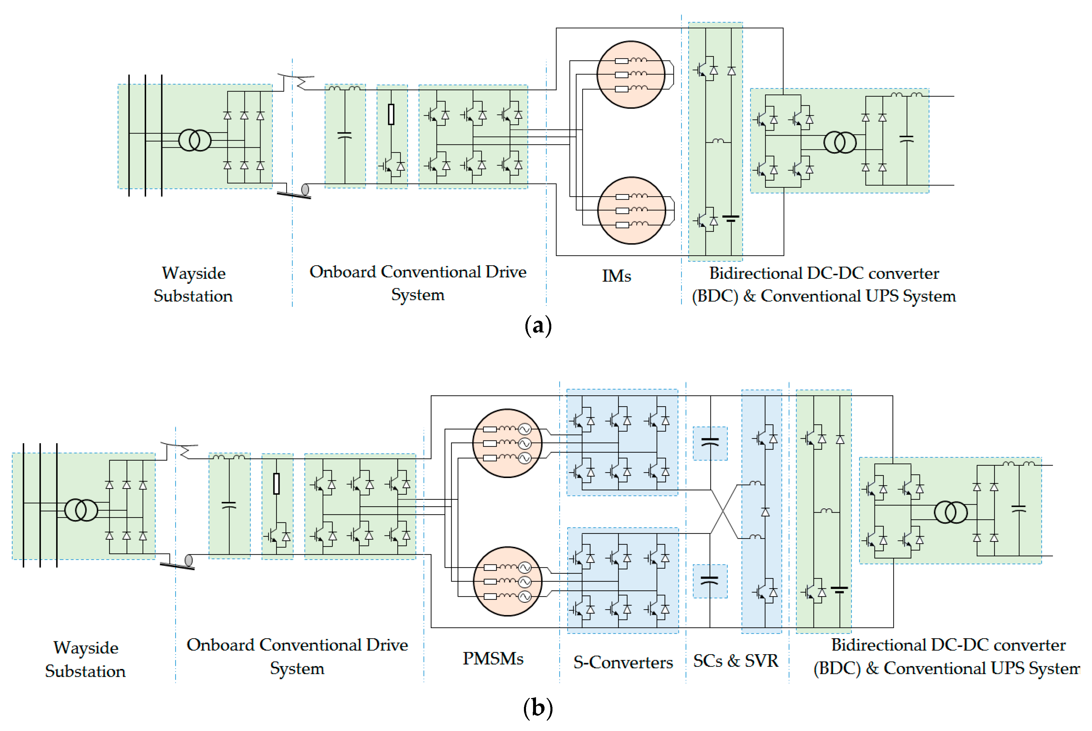
1.2. Propulsion System Topology

Electric propulsion systems can be categorized into two general types of single-machine propulsion systems and multi-machine propulsion systems. By using the single-machine type, the traction machine will be very large, and when the power requirement is low, the machine has to be working in either low-speed condition or low torque condition. On the other hand, a multi-machine drive (MMD) system is composed of two (or even more) small machines. Then, it can effectively share the load torque between the machines to avoid low-efficiency machine operation [16]. For example, when the power requirement is low, it can use a smaller number of its machines so that their maximum operating efficiency can be achieved. Moreover, this intrinsic redundancy of the MMD can be used to mitigate some effects of machine faults or converter failures [17]. Therefore, compared to the single-machine type, the MMD has better efficiency characteristics and higher reliability for the ET applications.

The most common MMD configurations being used in the railway tractions are based on two or more parallel-connected induction machines (IMs), which are supplied by one high-power converter [16,17]. In such a single-converter scheme of the MMD, some resources can be shared, and some power electronics and control parts can be removed, resulting in the reduction of cost, weight, and dimensions of the electric drive installation, in comparison to the multi-converter ones [16,17,18]. The efficiency of this topology can be more improved if the IMs are replaced with the Permanent Magnet Synchronous Machines (PMSMs) [19]. Since PMSMs allow the use of electric braking without requiring fully rated mechanical brakes for emergency use, this technology is currently in operation mostly for high-speed rail applications. However, driving parallel-connected PMSMs by the MMD having a single-converter topology leads to disruption of independent flux and torque control, because the same voltages and power switches must be applied to all machines [16,17,18,19]. In consequence, not only the load sharing cannot be accurately accomplished, but also a slight speed difference among the PMSMs (e.g., due to a small inequality of the wheels perimeters) causes an accumulative phase difference between angular positions of the machines, results in the desynchronization of them.

In the case of open-end winding (OEW) configuration, an OEW-PMSM can be powered by two separate converters [20]. The one that is connected between the winding-starts of the machine and the DC feeder is called F-converter, and the other which is attached between the winding-ends of the machine and the SC storages aboard the train is named S-converter in this paper. The flexibility of this configuration to supply machine windings from both two sides allows a variety of power flow control schemes that can be utilized to exchange energy between machines and the hybrid ES system [21]. Moreover, when multiple OEW-PMSMs are driven by an MMD system, one High-Power F-converter (HPF converter) can take the place of multiple F-converters. This HPF converter will be connected to the same sides of the windings in the traction machines. Then, the phase angles between the voltage vectors applied to the windings of each OEW-PMSM can be regulated by the S-converter, to which it is attached, independently of the others [22,23]. However, on the contrary, S-converters cannot be replaced with one high-power S-converter, since the F-converters have to be disabled during regenerative operation. Moreover, PMSMs cannot be connected in parallel with each other through the high-power S-converter during generator mode, due to the different situations for the adhesions and the slips that are between the wheels and the rail during train barking. Hence, this paper proposes that an OEW-PMSM, in combination with its own S-converter, which is attached to an SC bank, takes the place of each IM in an existent parallel-connected IMs based MMD in the existing train bogies, as shown in Figure 1a,b.

The machines can be upgraded only by replacing their old squirrel-cage rotors with new dedicated permanent magnet rotors without any changes in their stator structures and windings, at a minimal cost [23]. This restructuring enables the older ETs, which are currently in operation, to generate more propulsion power with an optimum efficiency over a wide speed range, resulting in more reliable transportation service. Furthermore, the battery circuit of the onboard UPS can be easily added to the suggested drive circuit to form the hybrid ES based propulsion system. Therefore, when the mains power fails or if input voltage fluctuations cause disturbing effects on the supply subsystems, the required traction energy can be provided immediately by the batteries, and then the train can continue to operate, although the control center will be alerted of these power source changes. Besides, to produce the required tractive torque during an emergency startup in such conditions, the SCs can effectively assist the drive system in providing the starting currents of traction machines, As a result, not only the propulsion system reliability but also the energy efficiency of regular ETs can be enhanced by implementing proposed restructuring strategy, as the advantage of both PMSMs with more power conversion density and the hybrid ESs comprising batteries and SCs can be taken. Furthermore, this topology can offer both the ability of the electric regenerative braking and multilevel operation that can increase the MMD functionality.

To control both speed and currents of each OEW-PMSM in the proposed MMD, an offline design in a cascade structure is provided for the control unit, which is planned based on the model predictive control (MPC) method.

1.3. PMSM Drive Control Based on Model Predictive Method

Due to recent advances in real-time signal processing, various methods of MPC have been developed and successfully applied to electric machine drive systems. The finite-set MPC technique uses a limited number of voltage vectors to evaluate the cost function. In general, some benefits of this approach are the simplicity of the design process, no need for voltage modulator, online relatively optimization, and simplicity in managing constraints and nonlinearities of the system [24]. However, the obtained voltage vector cannot result in an absolute minimum value of the cost function, even with a long calculation time or high switching frequency. Besides, system constraints do not effectively affect the process of designating a voltage vector as the control signal [25].

In another approach, the cost function is calculated through an optimal control method by considering the system model, system initial conditions, and some constraints on control variables and inputs [26]. Hence the control signals can be obtained as a continuous and precise analytical function. However, real-time solving of optimal control problems is time-consuming and results in a high volume of computation over each sampling time interval. In this regard, reference [27,28] used an optimization window to solve the constrained optimal control problem. The necessary condition to get an answer in this way is the reversibility of the Hessian matrix in each prediction horizon, whereas the calculation and evaluation of this matrix increase the computing time. Additionally, system constraints are examined after calculating the control signals in each control horizon, and by applying receding horizon control, this increases the probability that control signals exceed the constraints of the drive system. To solve these problems, researchers calculated the value of the Hessian matrix at the steady-state condition, though no optimal performance is observed in transient conditions.

In references [29,30], the active set method and the Hilderth’s method have been used in the PMSM drive system, to solve the online optimization problem, which both require considerable time to identify the active constraints. Recently, Bemporad et al. had presented the explicit linear quadratic optimization method for solving a constrained optimal control problem, in which the offline control signals are determined based on the position of control variables in the state-space polyhedron as a set of piecewise affine functions of the state variables vectors [31]. In this method, the trajectory of control variables is designed as a map, depending on the initial condition and the final state values of the system, so that this map leads to an optimal control path. Although, with any change in the steady-state conditions, the map will no longer be optimal. Reference [32] has applied this mapping method to control the speed of a PMSM in no-load conditions and showed that the computational speed can be greatly improved, however, under the predetermined conditions. In another application reference [33] used a trajectory map as a part of the cascaded control process to eliminate the offset error caused by the current sensors in the speed control of PMSM. Since finding control variables in the polyhedron is a time-consuming process, reference [34] provides some fast search strategies, although because of increasing the vector dimensions of control variables, determining the active area conditions in the polyhedral state-space will be more complex.

This paper presents a comprehensive algorithm for designing speed and current controllers of the proposed drive system with a cascaded structure in which the speed controller is performed based on the optimization window technique, and the current controller is designed on the basis of the Pontryagin maximum principle. These designs are not just for steady-state conditions, and the system constraints are also particularly effective in the process of generating control signals. The main novelty of the proposed algorithm is to generate control signals offline, and as a set of linear functions from the state variables and inputs, while the need for solving online optimization problems to find the optimal voltage vectors for the traction machine is eliminated. Therefore, the required memory size can be reduced to its minimum, and the microprocessor execution speed can be improved to its highest, which results in a lower level of online complexity and higher controller reliability. Moreover, the constraints on control signals can be checked separately to prevent the controller from mutual interferences, thus bringing significant savings in computing time. The feasibility of the control process in the real working conditions is vitally important. Therefore, the necessary and sufficient condition for generating control signals by the planned algorithm is also presented analytically.

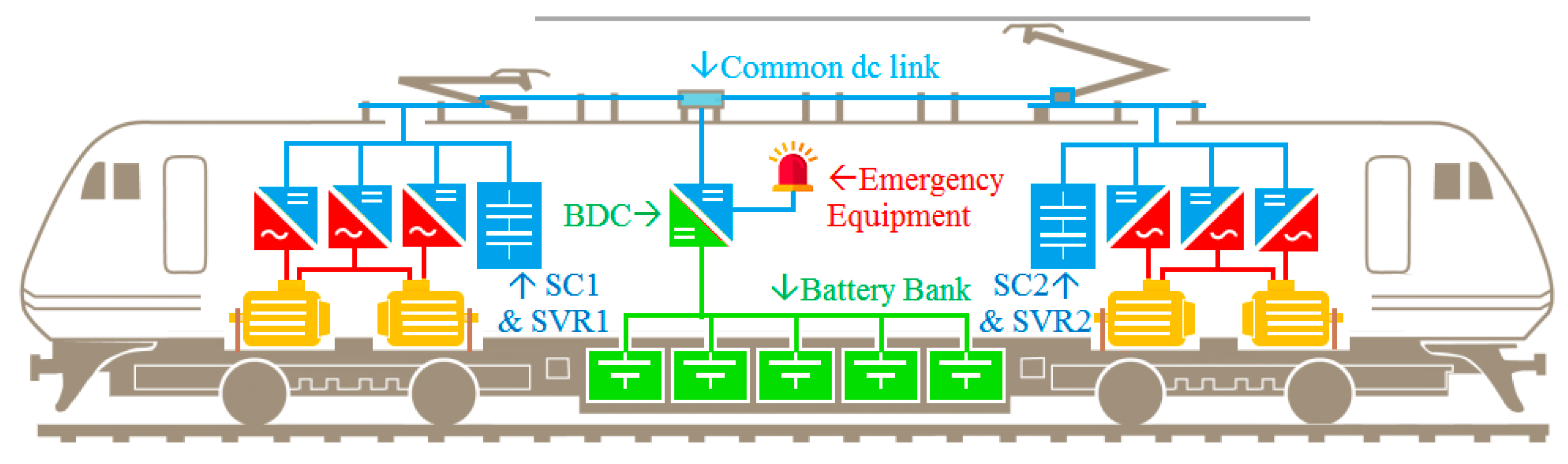
2. The Proposition of Modular MMD with Embedded UPS

Figure 1 illustrates the simplified circuit diagrams of both conventional and the suggested MMD systems with the UPS functionality. The suggested propulsion system of Figure 1b is easily expandable from both supply and storage sides, and it can be extended with more than two machines and developed by different machine types. Thus, it can be restructured as a coordinated multi-bogie propulsion system with a shared battery bank for the most electric railway wagons (and also for the DEMU locomotives), as it is shown in Figure 2. However, for the simplicity of description, a traction bogie with two similar open-winding surface-mounted PMSMs are considered to drive, in this paper. In such a traction bogie, each machine can be powered uninterruptedly by either the main feeder, the attached SCs, or the onboard battery backups, depending on the voltage values of these sources and the traction power demand situations.

2.1. The Power Management Method

As long as the wayside supply system works under normal conditions and the voltage of the transmission line is stable, the PMSMs are powered from the wayside power system, although in such conditions, the SCs can be used for the peak power assist. To balance the voltages of SCs, a bidirectional double-switch SC-voltage-regulator (SVR) is designed, by which each SC can be linked to the shared DC-link individually through its series inductor. Given the circuit structure of Figure 1b, the upper switch in the SVR circuit adjusts the voltage of the lower SC and vice versa, by applying a straight pulse width modulation (PWM) method, as a combined double DC-DC power converter. Besides, the backup batteries can be charged from the common DC-link through another bidirectional DC-DC converter (BDC), which has an additional power diode. This diode is connected between the positive input and the positive output terminals of the BDC, in a way that when the common DC-link voltage is below the battery bank voltage, the discharging current of batteries can directly flow through it while the diode is in forwarding bias.

The voltage levels of the three sources, i.e., the input feeder, the SCs, and the batteries, are set to be different from each other since their voltage levels determine which of these can feed the traction machines, through the three DC-AC converters. The supplying current flows from that source, which has the highest voltage level to the DC-AC converters of the traction drive. Hence, the reference voltage of the battery bank is considered to be under the minimum acceptable voltage level of the shared DC link. The voltage discharge ratio of the SCs is typically chosen to be about 50%, to utilize almost 75% of their stored energy. In some applications, this ratio is maintained higher than 50% for efficiency reasons, however in a hybrid ES configuration, the higher voltage discharge ratio of SCs results in the lower usability and functionality of the backup batteries. Hence, the reference voltage for the battery bank can be considered about 50% of the nominal voltage of the railway supply system, whereas the maximum voltage for the SCs can be defined by about 150% of the main supply voltage. For example, suppose that the voltages of SCs are higher than the other sources, e.g., due to a previous brake recovery charging action. Subsequently, they connect to the common DC link via the upper and the lower power diodes in the SVR. Thus, during the acceleration period of the train, the higher power for more tractive effort can be provided by the SCs. Then, after the starting acceleration, when the voltage level of SCs reaches the input feeder voltage, the traction load is automatically transferred to the main power source. In addition, if a power shortage occurs suddenly in the supply network or in the input feeder, again, the SCs can provide the traction power until their voltages are more than the voltage of the battery bank. In such a situation, if the period of the power outage is so long that the SCs voltages are reduced below the voltage value of battery bank, the power diode in BDC moves to the forward bias condition, and therefore, the lower voltage of battery bank appears across the common DC link spontaneously. During this situation, the BDC, which is a bidirectional converter, can also boost the battery voltage to compensate undesirable voltage drops and to maintain the voltage of DC-link at an acceptable level under different loading conditions, while in the period of boost operation, the power diode in the BDC switches to the reverse-biased naturally.

Each of these two machines can be supplied either by the shared high-power feeder-connected converter (the HPF converter), by its own SC-storage-connected converter (the S-converter) or from both sides through these two converters, depending on the difference between the angular rotor positions of the two machines. Each DC-AC converter module can be simply implemented by using a standard three-phase voltage source inverter (VSI) topology. All these VSI are supported by the main DC feeder, which is supplied by the wayside transformer-rectifier substation through the catenary wire or the third rail. However, only the S-converters have the duty to convert the recuperated energy to the stored energy in their SCs during braking and deceleration. Therefore, these converters must have the ability to work in bidirectional power mode, while the HPF converter only operates in the unidirectional power mode, although each of them has its own power rating. Since the HPF converter must have the ability to deliver full propulsion power to all traction machines simultaneously, it must be capable of withstanding the full driving currents in the worst operating conditions. The current rating for each S-converter is determined with regard to the maximum current stresses of the machine to which it is connected, whereas, the current rating for each S-converter is determined with regard to the maximum current stresses of the machine to which it is connected. Furthermore, the voltage rating of each converter can be decided based on its DC side voltage, i.e., their voltage ratings are 150% of the input feeder voltage.

The DC-link of each S-converter is directly coupled to its own SC, and when the SVR switches are turned off, both SCs are in series together and the charging current path is deviated to them through the middle power diode in the SVR circuit. In case of being more than two S-converters (for an MMD system with more than two machines), the SVR circuit can be easily expanded, or a combination of series-parallel connected SCs and batteries can be used to configure the hybrid ES bank. The SCs can support the peak power requested by the machines during start-up and acceleration states from the absorbed braking energy of train deceleration. Consequently, the inrush currents from the feeding system can be significantly reduced in the accelerating durations. The demanded power from the SCs can be directly injected to each machine through its S-converter, or it can be first transferred to the HPF converter through the SVR switches. Accordingly, in order to ensure that the active converters continuously perform their complementary functions well, the SVR circuit can manage the power flow between the supplying DC-link and the S-converters DC links in different operational states by providing proper switching action. In addition, the charging processes of the backup batteries at a constant current can be controlled by the BDC module independently based on their charging states.

2.2. Supplying Critical Devices Aboard the Train

To enhance the reliability of the power path to the critical items, including sensors and control devices, fire protection and emergency lights, and radio communications and signaling operations, they can be galvanically isolated from the common DC link in the power circuits through an additional dual-active-bridge (DAB) converter. This extra converter enables the voltage ratio adjustment for the sensitive loads as well, during different operational conditions of the drive system. This function is very important, especially when the voltage of batteries fluctuates, e.g., due to one or both motors being loaded in the absence of the main power supply. Moreover, a redundant DAB converter that directly connects some backup critical components to the batteries is recommended to eliminates potential single points of failure at an unlikely fault event in the drive converters. Through such a redundant interface, the emergency power can be activated for critical loads immediately by switching from the main supply system to the battery energy storage, directly and without interposed circuits.

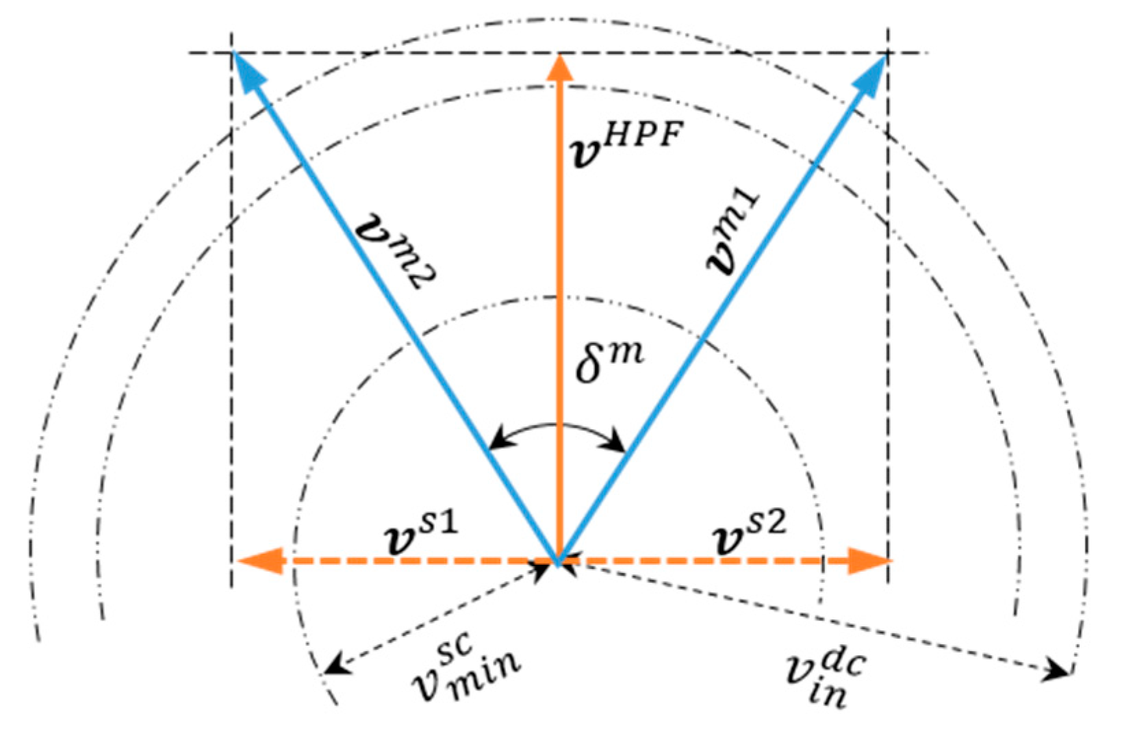
2.3. Extraction of Reference Voltages for DC-AC Converters

In the example traction drive of Figure 1b, the DC voltage across the common DC link is defined as $v_c^{dc}$ and the DC voltages across the SC-links that are connected to the S-converters of 1 and 2 are expressed as $v_1^{sc}$ and $v_2^{sc},$ respectively. Owing to the existence of middle power diode in the SVR circuit, it is clear that the following inequality holds true, spontaneously:

$$v_c^{dc}\le v_1^{sc}+v_2^{sc},$$

(1)

Moreover, by applying proper switching patterns to the SVR switches, the values of $v_1^{sc}$ and $v_2^{sc}$ are expected to be equal to each other in all conditions. It should be noted that both $v_1^{sc}$ and $v_2^{sc}$ can increase by more than the input feeder voltage of $v_{in}^{dc}$, because they will be amplified under regenerative braking conditions. The maximum DC side voltage of the three DC-AC converters, i.e., $v_c^{dc}$, $v_1^{sc}$ and $v_2^{sc}$, is considered to be increased up to 1.5$v_{in}^{dc}$, since the maximum charge-discharge ratio of SCs is allowed to reach 50%. Furthermore, it is presumed that both machines have identical ratings, and all converters have similar circuit topology with the same voltage ratings. Each machine coil is powered by two VSIs with an angle difference between their voltage vectors, and therefore, the current vector of the machine coils cannot be at the same phase angle as their voltage vectors of these two converters, at the same time. Hence, providing reactive power is essential for both S-converters. Although the average voltage level of an SC might not be affected by the amount of reactive power provided by its own S-converter [35], this power component can cause voltage fluctuation especially during high current demand at acceleration or braking periods. In such situations also, the SVR circuit can be used to tackle this problem and eliminate the AC side resulting harmonics. As a result, since the SVR switches can regulate the voltage of SC-links in different operational states, voltages of all machine windings can be adjusted through the two side converters, independently of each other.

The diagram of voltage vectors and current vectors for all AC parts in the sample MMD circuit of Figure 1b is shown in Figure 3. Given this diagram, the voltage vector of $\overrightarrow{v^{mx}}$ which is for the windings in the traction machine of x (x = 1 and 2) is equal to:

$$\overrightarrow{v^{mx}}=\overrightarrow{v^{HPF}}-\overrightarrow{v^{sx}}$$

(2)

wherein this equation, $\overrightarrow{v^{HPF}}$ represents the AC side voltage vector of the HPF converter, and this vector is taken as the reference vector of the drive system. In addition, $\overrightarrow{v^{sx}}$ stands for the voltage vector of the S-converter, which is coupled to the machine x.

In synchronous rotating reference frame, and at the angular speed of ${\omega }_s$ these vectors can be expressed as follows:

$$\overrightarrow{v^{mx}}=\left[\begin{array}{c}{v}_q^{mx}\\ v_d^{mx}\end{array}\right],\overrightarrow{v^{HPF}}=\left[\begin{array}{c}{v}_q^{HPF}\\ v_d^{HPF}\end{array}\right],\overrightarrow{v^{sx}}=\left[\begin{array}{c}{v}_q^{sx}\\ v_d^{sx}\end{array}\right],$$

(3)

wherein Equation (3), $v_d^k$ and $v_q^k$ represent d-axis and q-axis components for the voltage vector of $\overrightarrow{v^k}$. Due to the possible difference in the angular position of the two rotors, the traction machines may not have identical voltage vectors, even with equal torques and speeds. Furthermore, a very slight speed difference is inevitable because of any possible trifling difference between mechanical power transmission systems of the two machines or moving of a defective wheel in the bogie with a minor different speed and axle load. Thus, the angle difference between the voltage vectors of the two machines (${\delta }^m$) may be varying during every running condition. Nonetheless, these variations in the angles difference are not fast enough to cause a frequency difference between the HPF converter and the S-converters. This circumstance can be expressed as follows:

$$\frac{d}{dt}{\delta }^m<\frac{4\pi }{P}$$

(4)

where P is the number of poles and ${\delta }^m$ is in radian. Therefore, the duty of feeding active power to a traction machine may alternate between the attached DC-AC converters on both sides of that machine. To determine the voltage vector of each converter, at first the voltage vector of $\overrightarrow{v^{mx}}$ for its connected machine is calculated based on its load torque and its reference speed, as described in the control section. Then, the reference vector of $\overrightarrow{v^{HPF}}$ is considered to be in parallel with, and in the same direction as the interior angle bisector of vectors $\overrightarrow{v^{m1}}$ and $\overrightarrow{v^{m2}}$. Afterward, the voltage vectors of $\overrightarrow{v^{s1}}$ and $\overrightarrow{v^{s2}}$ are decided to be perpendicular to the $\overrightarrow{v^{HPF}}$ in such a way that they are at a straight angle to each other. As a consequence, the propulsion power can be evenly balanced between the two machines. Actually, the S-converters regulate the torque angle (the angle between the stator and rotor fields) of their connected machines to the proper value, so that the mechanical load can be divided equally between them. Besides, the amplitudes of $\overrightarrow{v^{HPF}}$ and each $\overrightarrow{v^{sx}}$ can be obtained from Equation (2), even though they also may be modified based on the active and reactive powers regulation process by the drive control unit. The output voltage of the drive converters is adjusted by the voltage divider (VD) block in the control unit, based on the abovementioned philosophy.

The main objective of the MMD system is the torque and speed regulation of the traction machines in response to the operational commands and signals from the train control systems. It can be achieved by managing the flow of power through the MMD drive converters, as described in the next section in detail.

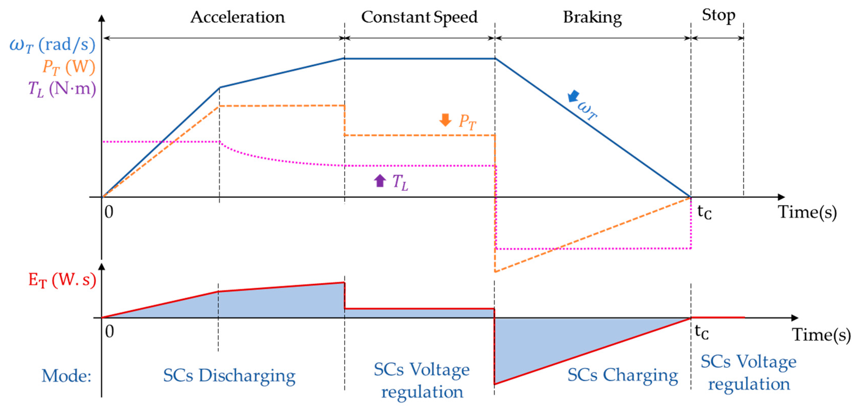
3. Energy Management Strategy

Different operation conditions of the suggested MMD system can be separated into four states. The propulsion system can generate low and high constant speeds, acceleration, and regenerative deceleration. The practical operation of the drive system might be complex, but it is a combination of the aforementioned four states. These operating states can be defined as follows:

3.1. Soft Acceleration at Motoring State

This operating state is selected during the normal run and slow accelerations of the train when the required power for both traction machines is below the power limit that is planned for the main DC feeder ($p_{min}^{in}$). In this state, the SCs are neither absorbing nor providing active power to the traction machines, although, these capacitors can be exploited for delivering requisite reactive power to the traction machines. Therefore, both SVR switches are off, and the SCs links disconnected from the common DC link. Since the SCs voltages are higher than the voltage level of the backup batteries, the power diode in BDC is reversely biased, and no energy flows from batteries to the AC-DC converters, unless a power interruption happens in the input feeder. In such circumstances, both SVR and BDC circuits will be activated and provide the traction power based on the described strategy.

Moreover, in the low power condition, it will also be possible to involve only one machine (or a smaller number of machines in case more than two machines are employed) while the other machine is disabled by its S-converter. Implementing such a split traction control in the low power periods lets the active machine be more energy-efficient, and then the overall efficiency of the MMD can improve.

3.2. Fast Acceleration at Motoring State

This operating state is decided during the train start-up and rapid acceleration when the traction machines require a power amount higher than the $p_{min}^{in}$. During such boost starts, the SCs can assist in providing more power to fulfill the requested peak power by traction machines to avoid high power transient demand from the main power supply, preventing high inrush currents from the supplying-rectifier substation. In such conditions, machine windings can absorb both active and reactive powers from the two connected converters on their sides.

Besides, with a proper phase-shift in the switching carrier signals of those converters, an equivalent doubled switching frequency can be achieved to reduce the current ripples, to keep the high-current switching-harmonics at an acceptable level. Furthermore, during the power interruptions, both SCs and batteries can provide the traction power, however, with a bounded acceleration and an optimal speed trajectory.

3.3. Regenerative State

In the duration of train deceleration or braking, only the S-converters are modulated to restore the converted kinetic energy coming from the traction machines to their connected SCs. To prevent any voltage fluctuations on the common DC link or on the feeder side, no energy is returned to the supply side in this period, by turning the SVR switches off.

When continuous regenerative braking is needed, to make sure that the voltages of SCs are within the safe operating range, the BDC operates in buck mode simultaneously, to transfer the excess energy from the SCs to the batteries. Nonetheless, to extend the life of batteries, and to increase the accuracy of battery state-of-charge estimation, it is recommended that when designating the hybrid ES components, they are properly sized to prevent such situations.

3.4. Neutral Moving and Stop States

In the period of stop mode, when no energy conversion is needed to be performed by the traction machines, no converter is required to commutate. However, to prepare the SCs for the next starting acceleration, the charging state can be enabled for them in this duration, through the SVR switches. Besides, during normal train run, the charge management and the voltage stabilization of the ES components can be accomplished by the SVR and the BDC circuits, independent of machine windings currents. Since the balancing energy can be directly conveyed between the DC feeder and the ES components, without drawing any zero sequence currents through the machine windings, the power losses in the motor windings are reduced, and the machine magnets are protected from demagnetization [36].

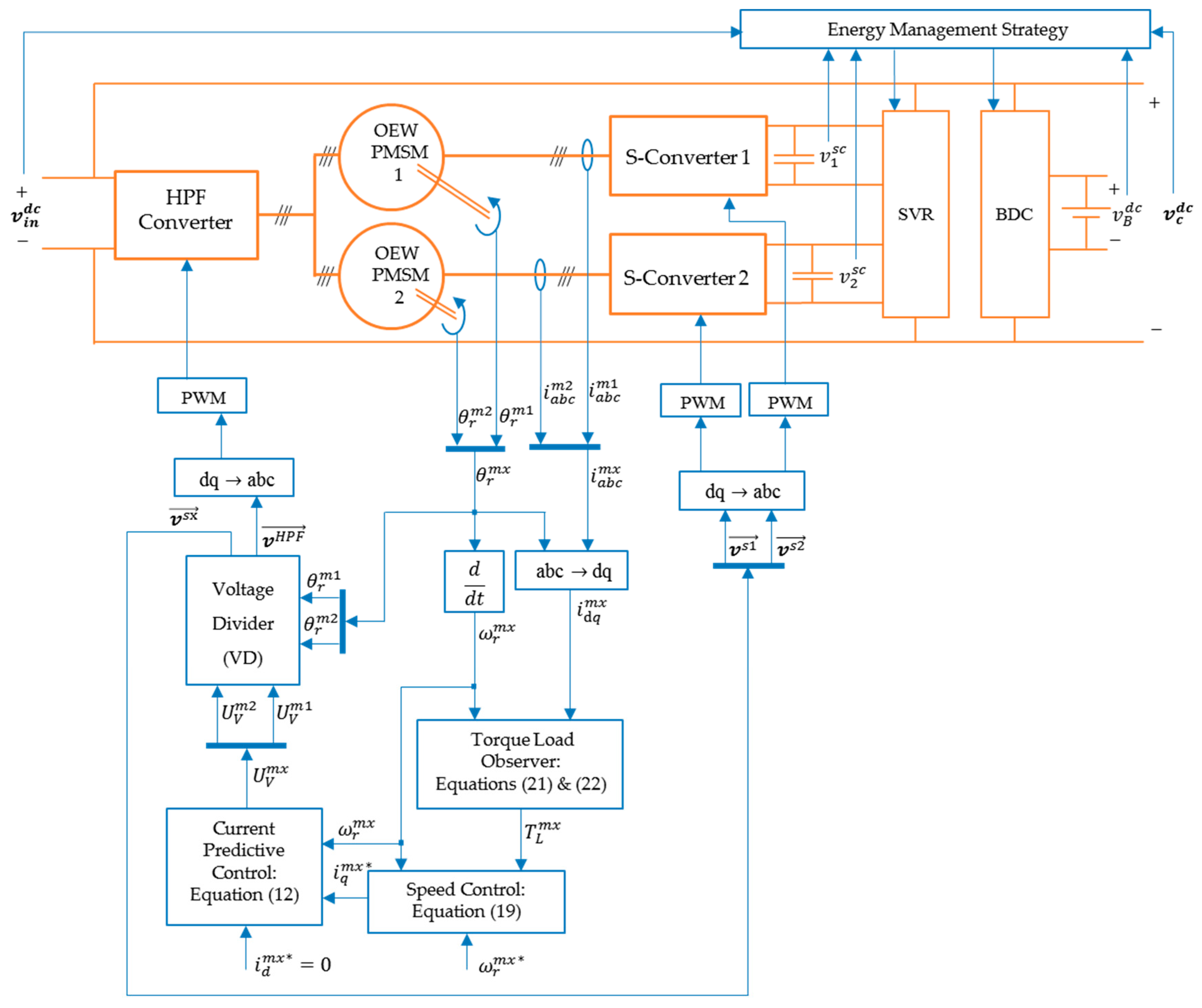
4. Proposed Methodology for Speed and Current Controllers

A model-based optimal control method for the real-time speed regulation of each PMSM is proposed in this section. The goal of this control strategy is to provide an optimal amount of torque that allows driving each PMSM at the desired speed profile, as required by the train control system while satisfying both voltage and current constraints. As presented in Figure 4, the architecture of the proposed control method consists of an outer loop that controls the mechanical dynamics and an inner loop that regulates the electrical components of each machine. The current constraints are checked in the outer loop by limiting maximum torque that can be produced by each machine, and voltage constraints are considered in the inner loop based on voltage requirements and limitations for each converter. Therefore, the voltage and current constraints can be separately evaluated and satisfied, and then the performance of the controller is not affected by mutual interferences between them.

4.1. Mathematical Modelling of OEW-PMSMs

A brief overview of the mathematical model for the three-phase open-end-wiring PMSM with a sinusoidal winding distribution on the stator and a number of permanent magnets on the rotor, in the synchronous rotating frame, is presented in this part.

The electrical equations for this machine can be expressed as follows:

$$\frac{d}{dt}\left[\begin{array}{c}{i}_q^{mx}\left(t\right)\\ i_d^{mx}\left(t\right)\end{array}\right]=\left[\begin{array}{cc}-\frac{r_s}{L}& -{\omega }_r^{mx}\left(t_i\right)\\ {\omega }_r^{mx}\left(t_i\right)& -\frac{r_s}{L}\end{array}\right]\left[\begin{array}{c}{i}_q^{mx}\left(t\right)\\ i_d^{mx}\left(t\right)\end{array}\right]+\left[\begin{array}{cc}\frac{1}{L}& 0\\ 0& \frac{1}{L}\end{array}\right]\left[\begin{array}{c}{v}_q^{mx}\left(t\right)\\ v_d^{mx}\left(t\right)\end{array}\right]+\left[\begin{array}{c}-\frac{{\psi }_f}{L}\\ 0\end{array}\right]{\omega }_r^{mx}\left(t_i\right)$$

(5)

where $L_d$ and $L_q$ are the stator inductances in (H) on the d-axis and the q-axis respectively, $r_s$ is the stator resistance in (Ω), and ${\psi }_f$ is the magnetic flux produced by rotor magnets in (Wb). These constant values are the same for both PMSMs. In addition, ${\omega }_r^{mx}$ is the electrical rotor speed in (rad/s), $i_q^{mx}$ and $i_d^{mx}$ are the stator currents in (A) and $v_q^{mx}$ and $v_d^{mx}$ are the stator voltages in (V), on q-axis and d-axis respectively, for the machine x (x = 1 and 2). The mechanical dynamics of each machine can be described by the following equations:

$$\frac{d}{dt}\left({\omega }_r^{mx}\left(t\right)\right)=\frac{2}{p{J}_{}}\left(T_e^{mx}-T_L^{mx}\right)-\frac{B_m}{J_{}}{\omega }_r^{mx}\left(t\right),$$

(6)

$$\frac{d}{dt}\left({\theta }_r^{mx}\left(t\right)\right)={\omega }_r^{mx}\left(t\right),$$

(7)

where ${\theta }_r^{mx}$ is the rotor position in (rad), as well as $T_L^{mx}$ and $T_e^{mx}$ are the load and electrical torques in (N⋅m), respectively, for the machine x. Moreover, p is the total number of poles, J is the inertia coefficient in (kg.m²), $B_m$ is the coefficient of viscous friction in (N⋅m.s). These constant values are the same for both PMSMs as the two machines are identical. In addition, the electrical torque $T_e^{mx}$, which is consists of the electromagnetic and the reluctance components, can be written as follows:

$$T_e^{mx}=\frac{3}{2}\frac{p}{2}\left({\psi }_f+\left(L_d-L_q\right)i_d^{mx}\left(t\right)\right)i_q^{mx}\left(t\right),$$

(8)

The effects of core saturation and cogging torque are neglected, and it is assumed that the magnets are mounted on the surface of the rotor, therefore $L_d=L_q=L$.

4.2. Current Predictive Control

To design current predictive control, the state-space model of Equation (5) is used. Then let us rewrite Equation (5) as the following equations:

$$\frac{d}{dt}{X}_I^{mx}\left(t\right)=A\left(t_i\right)X_I^{mx}\left(t\right)+B{U}_V^{mx}\left(t\right)+D{\omega }_r^{mx}\left(t_i\right),$$

(9)

$$X_I^{mx}\left(t\right)={\left[\begin{array}{cc}{i}_q^{mx}\left(t\right)& i_d^{mx}\left(t\right)\end{array}\right]}^T,$$

(10)

$$U_V^{mx}\left(t\right)={\left[\begin{array}{cc}{v}_q^{mx}\left(t\right)& v_d^{mx}\left(t\right)\end{array}\right]}^T,$$

(11)

where $X_I^{mx}\left(t\right)$ and $U_V^{mx}\left(t\right)$ are the state vector and the control signals, respectively. The speed variable of ${\omega }_r^{mx}\left(t_i\right)$ is the rotor speed which is measured as the state feedback at the time of $t_i$, and the control signals are designed to drive the machine from its current condition at $t_i$ to the desired condition at $t_{\left(i+1\right)}$. During this tiny time interval, ${\omega }_r^{mx}$ is assumed to be constant, then the control signals can be matched in the state-space model of the machine x, in this duration.

The feedback controller is intended to force the actual machine currents to track the current references, with the lowest required voltages provided by related converters. Hence, the following performance index is constructed to minimize with respect to Equation (5), as:

$$\begin{array}{cc}\hfill {\mathcal{J}}_I=& \underset{U_V^{mx}}{\min }\left\{\frac{1}{2}\right[{\left(X_I^{mx}\left(t_f\right)-X_I^{mx}{}^{*}\right)}^T{Q}_f\left(X_I^{mx}\left(t_f\right)-X_I^{mx}{}^{*}\right)\hfill \\ \hfill & +{{\displaystyle \int }}_{t_i}^{t_f}\left[{\left(X_I^{mx}\left(\tau \right)-X_I^{mx}{}^{*}\right)}^{T}Q\left(X_I^{mx}\left(\tau \right)-X_I^{mx}{}^{*}\right)+U^T\left(\tau \right)RU\left(\tau \right)\right]d\tau \left]\right\},\hfill \end{array}$$

(12)

$$\tau \in \left[t_i,t_i+t_f\right],$$

(13)

in which the $t_f$ is the final time of the prediction horizon, and $X_I^{mx}{}^{*}$ is the desired value of state variables at $t_f$. The weight matrices of $R$, $Q$ and $Q_f$ are chosen so as to be diagonal and positive definite. These matrices can be tuned based on the designer’s experience or by using constructive techniques [37].

To find the desired voltage vector of $U_V^{mx}\left(t\right)$, the above optimal problem is solved based on the Pontryagin maximum principle [38] as described in Appendix B. Then, by applying necessary optimality condition, first-order state equations are:

$$\frac{d}{dt}\left[\begin{array}{c}{i}_q^{mx}\left(t\right)\\ i_d^{mx}\left(t\right)\end{array}\right]=\left[\begin{array}{cc}-\frac{r_s}{L}& -{\omega }_r^{mx}\left(t_i\right)\\ {\omega }_r^{mx}\left(t_i\right)& -\frac{r_s}{L}\end{array}\right]\left[\begin{array}{c}{i}_q^{mx}\left(t\right)\\ i_d^{mx}\left(t\right)\end{array}\right]-\left[\begin{array}{cc}\frac{1}{L}& 0\\ 0& \frac{1}{L}\end{array}\right]\left[\begin{array}{cc}\frac{1}{R_{11}}& 0\\ 0& \frac{1}{R_{22}}\end{array}\right]\left[\begin{array}{cc}\frac{1}{L}& 0\\ 0& \frac{1}{L}\end{array}\right]\left[\begin{array}{c}{\lambda }_1\left(t\right)\\ {\lambda }_2\left(t\right)\end{array}\right]+\left[\begin{array}{c}-\frac{{\psi }_f}{L}{\omega }_r^{mx}\left(t_i\right)\\ 0\end{array}\right]$$

(14)

where the covector $\lambda ={\left[\begin{array}{cc}{\lambda }_1\left(t\right)& {\lambda }_2\left(t\right)\end{array}\right]}^T$ can be obtained by the following equation:

$$\frac{d}{dt}\left[\begin{array}{c}{\lambda }_1\left(t\right)\\ {\lambda }_2\left(t\right)\end{array}\right]=-\left[\begin{array}{cc}{Q}_{11}& 0\\ 0& Q_{22}\end{array}\right]\left(\left[\begin{array}{c}{i}_q^{mx}\left(t\right)\\ i_d^{mx}\left(t\right)\end{array}\right]-\left[\begin{array}{c}{i}_q^{mx}{}^{*}\left(t\right)\\ i_d^{mx}{}^{*}\left(t\right)\end{array}\right]\right)-\left[\begin{array}{cc}-\frac{r_s}{L}& {\omega }_r^{mx}\left(t_i\right)\\ -{\omega }_r^{mx}\left(t_i\right)& -\frac{r_s}{L}\end{array}\right]\left[\begin{array}{c}{\lambda }_1\left(t\right)\\ {\lambda }_2\left(t\right)\end{array}\right],$$

(15)

Afterward, by using the forward Euler discretization in time, the machine voltages as the control signals at every time step of h (where h is equal to $h=t_{i+1}-t_i$) are:

$$U_V^{mx}\left(t_i\right)=-R^{-1}{B}^{T}K\left(\left(M^{-1}\left[\left(I+A\left(t_i\right)h\right)X_I^{mx}\left(t_i\right)+hD+\left(B{R}^{-1}{B}^{T}h\right)K{X}_I^{mx}{}^{*}\right]\right)-X_I^{mx}{}^{*}\right),$$

(16)

that $K=\left[\left(I+A^T\left(t_i\right)h\right)Q_f+Qh\right]$ and the matrix M is equal to:

$$M=\left[\begin{array}{cc}1+\left(\frac{Q_{11}}{R_{11}}+\left(\frac{1}{h}-\frac{r_s}{L}\right)\frac{Q_{f11}}{R_{11}}\right){\left(\frac{h}{L}\right)}^2& \frac{Q_{f22}}{R_{22}}{\left(\frac{h}{L}\right)}^2{\omega }_r^{Mx}\left(t_i\right)\\ -\frac{Q_{f11}}{R_{11}}{\left(\frac{h}{L}\right)}^2{\omega }_r^{Mx}\left(t_i\right)& 1+\left(\frac{Q_{22}}{R_{22}}+\left(\frac{1}{h}-\frac{r_s}{L}\right)\frac{Q_{f22}}{R_{22}}\right){\left(\frac{h}{L}\right)}^2\end{array}\right]$$

(17)

matrix $M$, it is necessary to consider the conditions in which the determinant of M is greater than zero. The determinant of M can be expressed as follows:

$$\mathrm{Det}\left(M\right)=\left(1+\left(\frac{Q_{11}}{R_{11}}+\left(\frac{1}{h}-\frac{r_s}{L}\right)\frac{Q_{f11}}{R_{11}}\right){\left(\frac{h}{L}\right)}^2\right)\left(1+\left(\frac{Q_{22}}{R_{22}}+\left(\frac{1}{h}-\frac{r_s}{L}\right)\frac{Q_{f22}}{R_{22}}\right){\left(\frac{h}{L}\right)}^2\right)+\frac{Q_{f11}}{R_{11}}\frac{Q_{f22}}{R_{22}}{\left(\frac{h}{L}\right)}^4{\omega }_r^{Mx}{}^2\left(t_i\right)$$

(18)

Given that the $\mathrm{Det}\left(M\right)$ must always be greater than zero, it is observed that h must set to be smaller than the electric time constant of the PMSM, which is under controlled, ($h<\frac{L}{r_s}$). Therefore, since the determinant of matrix M can always be positive, the matrix reversibility of M can be proved, and the unique control signals are always achievable. Moreover, if the voltage vector of $U_V^{mx}\left(t\right)$ exceed the predetermined constraint, the rated converter voltage is replaced with the set of calculated command to satisfy the voltage constraints.

4.3. Speed Predictive Control

The speed controller regulates the torque component of the current command, $i_q^{mx}{}^{*}\left(t\right)$, by evaluating machine acceleration and kinetic energy as the control variables. Besides, the flux producing component of the current command, $i_d^{mx}{}^{*}$, is forced to zero to maximize the torque density of the traction machine [39]. Any change in the speed command or feedback, during machine acceleration or deceleration, causes electric power oscillations in the drive system. Therefore, to ensure the speed reaches its reference value, while the power fluctuations and speed variations are minimized, a performance index is defined for speed regulator as follows:

$${\mathcal{J}}_S=\underset{{\omega }_r^{•x}}{min}\left\{\frac{1}{2}{{\displaystyle \int }}_{t_i}^{t_f}\left[{\left(X_S^{mx}{}^{*}-X_S^{mx}\left(\tau \right)\right)}^T{Q}_S\left(\tau \right)\left(X_S^{mx}{}^{*}-X_S^{mx}\left(\tau \right)\right)\right]d\tau \right\}$$

(19)

wherein this equation, $X_S^{mx}\left(\tau \right)={\left[\begin{array}{cc}{\omega }_r^{•x}\left(\tau \right)& E_c^{mx}\left(\tau \right)\end{array}\right]}^T,X_S^{mx}{}^{*}={\left[\begin{array}{cc}0& \frac{1}{2}\end{array}(J_t^{mx}){\left({\omega }_r^{mx}{}^{*}\left(t\right)\right)}^2\right]}^T$ and also ${\omega }_r^{•x}\left(\tau \right)=\frac{d}{dt}\left({\omega }_r^{mx}\left(\tau \right)\right)$. Also $E_c^{mx}$ is the kinetic energy, ${\omega }_r^{•x}\left(\tau \right)$ is the slope of the angular speed and $J_t^{mx}$ is the total moment of inertia (i.e., the load inertia plus the machine inertia) for machine x. With considering $Q_S$ as a positive definite weighting matrix, and after simplifying Equation (19) it can be described as follows:

$$\begin{array}{c}{\mathcal{J}}_S=\underset{{\omega }_r^{•x}}{min}\left\{\frac{1}{2}{{\displaystyle \int }}_{t_i}^{t_f}\right[Q_S^{1,1}{\left({\omega }_r^{•x}\left(\tau \right)\right)}^2-{\omega }_r^{•x}\left(\tau \right)\left(Q_S^{1,2}\left(\tau \right)+Q_S^{2,1}\left(\tau \right)\right)\left(E_c^{mx}{}^{*}-E_c^{mx}\left(\tau \right)\right)+\\ Q_S^{2,2}\left(\tau \right){\left(E_c^{mx}{}^{*}-E_c^{mx}\left(\tau \right)\right)}^2\left]d\tau \right\},\end{array}$$

(20)

Minimizing this integral cost function concerning the speed slope of ${\omega }_r^{•x}$ results in the optimal speed slope as follows:

$$\left(\frac{Q_S^{1,1}}{Q_S^{1,2}\left(t\right)+Q_S^{2,1}\left(t\right)}\right){\omega }_r^{•x}\left(t\right)=\frac{2J_t}{p^2}\left({\left({\omega }_r^{mx}{}^{*}\left(t_i\right)\right)}^2-{\left({\omega }_r^{mx}\left(t_i\right)\right)}^2\right)$$

(21)

where ${\omega }_r^{mx}{}^{*}\left(t_i\right)$ and ${\omega }_r^{mx}\left(t_i\right)$ are the reference and the measured angular speeds for machine x, respectively. If the elements of the weight matrix of $Q_S$ in Equation (21) are chosen as:$Q_S^{1,2}\left(t\right)=\frac{2}{p}\mathrm{\Delta }{t}^2$, $Q_S^{2,1}\left(t\right)=\frac{1}{2T_L\left(t_i\right)}$, and $Q_S^{2,2}$ being an arbitrary value, then $Q_S$ is a positive definite matrix, and Equation (21) can be rewritten as follows:

$$\frac{2}{p}{\omega }_r^{•x}\left(t\right)T_L\left(t_i\right)\mathrm{\Delta }{t}^2=\frac{2J_t}{p^2}\left({\left({\omega }_r^{mx}{}^{*}\right)}^2-{\left({\omega }_r^{mx}\left(t_i\right)\right)}^2\right)$$

(22)

By applying the PMSM mechanical equations of (6), (7), and (22) to the electrical torque equation of (8), the torque component of stator current command can be found as follows:

$$i_q^{mx}{}^{*}\left(t_i\right)=\frac{8J.J_t^{mx}}{\mathrm{\Delta }{t}^2.3.p.{\psi }_f.T_L^{mx}\left(t_i\right)}\left({\left({\omega }_r^{mx}{}^{*}\right)}^2-{\left({\omega }_r^{mx}\left(t_i\right)\right)}^2\right)+\frac{8.B_m}{3.p^2.{\psi }_f}{\omega }_r^{mx}\left(t_i\right)+\frac{4}{3.p.{\psi }_f}{T}_L^{mx}\left(t_i\right)$$

(23)

When $i_q^{mx}{}^{*}$ exceeds its predetermined constraint, the rated current value is replaced with the calculated command, and therefore, the current constraints are satisfied independently. Consequently, the speed changes only affect the current command, and the voltage constraints are independently limited by the current controller loop.

4.4. Torque Estimation Process

The load torque can be estimated by considering the mechanical machine model, introduced by Equations (6) to (8), and it can be rewritten as follows:

$$T_L^{mx}=\frac{3}{2}\frac{p}{2}{\psi }_f.i_q^{mx}{\left(t\right)}_{}-J{\frac{2}{p_{}}}_{}\frac{d}{dt}\left({\omega }_r^{mx}\left(t\right)\right)-B_m\frac{2}{p}{\omega }_r^{mx}\left(t\right)$$

(24)

Then, by using the Backward Euler Approximation, as an implicit method for time discretization of differential equations, Equation (24) can be rewritten as follows:

$$T_L^{mx}\left(t_i\right)=\frac{3}{2}\frac{p}{2}{\psi }_f.i_q^{mx}{\left(t_i\right)}_{}-J{\frac{2}{p_{}}}_{}\left(\frac{{\omega }_r^{mx}\left(t_i\right)-{\omega }_r^{mx}\left(t_{i-1}\right)}{h}\right)-B_m\frac{2}{p}{\omega }_r^{mx}\left(t\right),$$

(25)

To increase the accuracy of discretization in the implementation, the parameter of $T_L^{mx}$ is set to the average value of its 10 previous samples as follows:

$$T_L^{mx}\left(t_i\right)=\frac{1}{10}{{\displaystyle \sum }}_{z=0}^{10}{T}_L^{mx}\left(t_{i-z}\right)$$

(26)

Besides, the mechanical parameters of $B_m$ and $J$ in Equation (25) can be calculated based on an online estimation method proposed in [40], which does not need the aid from the nominal and measured values of PMSM parameters. Therefore, the torque estimation procedure does not suffer from external disturbances and the mismatching of other machine parameters.

4.5. Impacts of Constraints on the Controller Performance

If a unified MPC strategy has been designed for the proposed drive system, the three state variables of $i_d^{mx}$,$i_q^{mx}$ and ${\omega }_r^{mx}$ for each PMSM have to be controlled by the two control signals of $v_d^{mx}$ and $v_q^{mx}$. In such circumstances, the control signals are highly dependent on the machine speed, and any change in the speed command can cause large variations for both $v_d^{mx}$ and $v_q^{mx}$. Then, when the speed command changes, these control signals are continually confined to their upper and lower bounds by the defined system constraints, and this will cause the controller to deviate from the optimal path. To overcome this issue, most previous studies suggested that a PI controller, as a part of the cascade control process, determined $i_q^{mx}$ command. However, in this mode, only the error between the reference and the measured speed value reaches zero, regardless of the energy amount which is required to change the speed, and irrespective of the appropriate speed gradient to produce proper dynamic behavior for the machine. Therefore, the command signals may have unpredictable oscillations, and still, the controller cannot provide the optimal path for the state variables [33].

In the described proposed MPC, the command $i_q^{mx}{}^{*}$ is adjusted based on the value of changes in the speed command, and the speed gradient at each sampling interval is determined as a fraction of maximum allowable kinetic energy. The controller serves the minimum time to reach the final value by optimizing the speed gradient based on the designated cost function. When the calculated speed gradient is so fast that the speed cannot reach the specified value within the very short period of switching time, the nominal current limit will be selected, which means that the controller uses the rated capacity of the machine. Thus, the machine will not be over-powered, and at the same time, the speed fluctuations will be eliminated because the limitations of both kinetic energy and winding currents are considered in the control procedure. As a result, no significant fluctuations will be observed, and when the current command is limited by the system constraints, the resulting command will be the best possible way to change the machine speed.

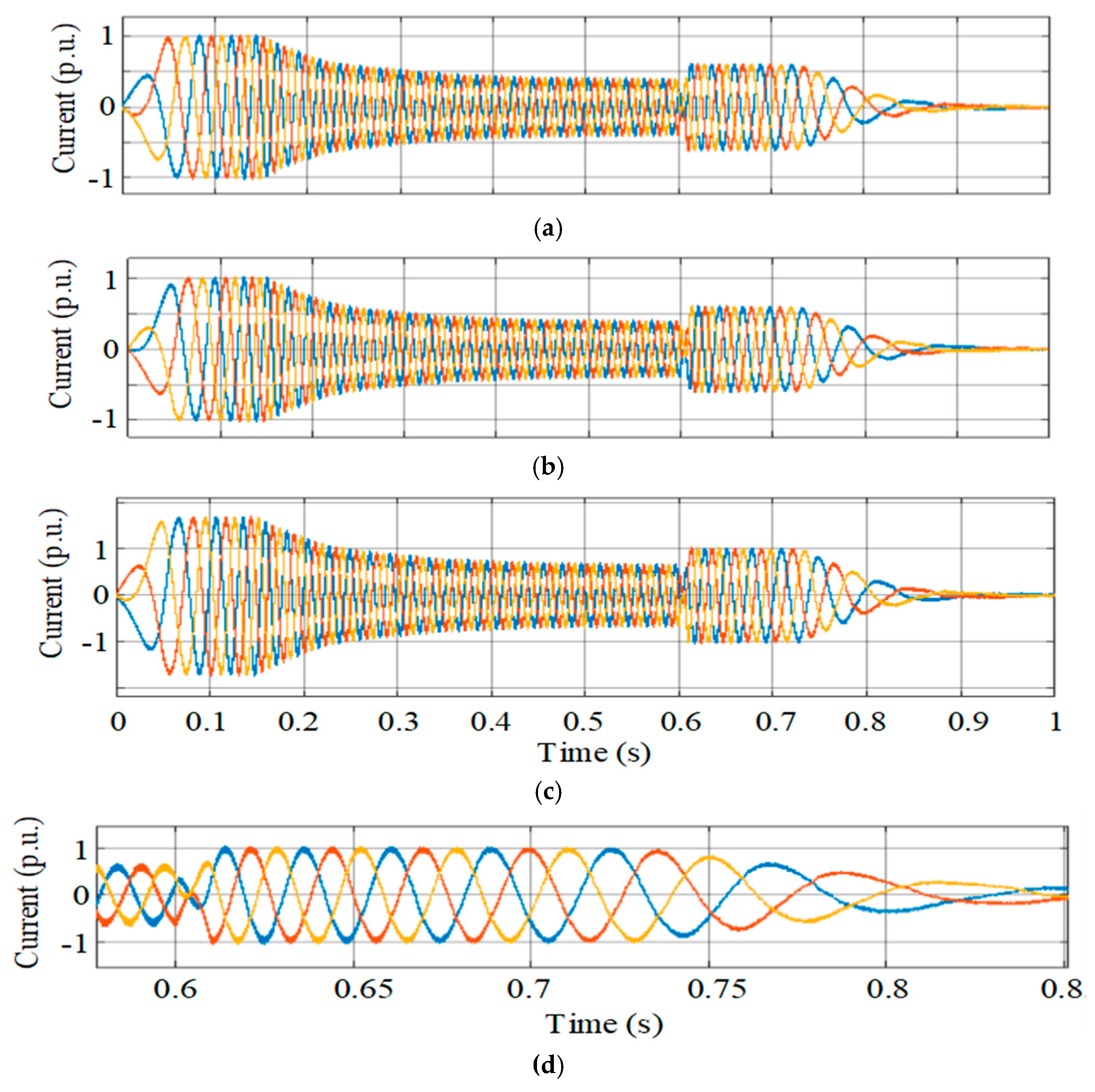
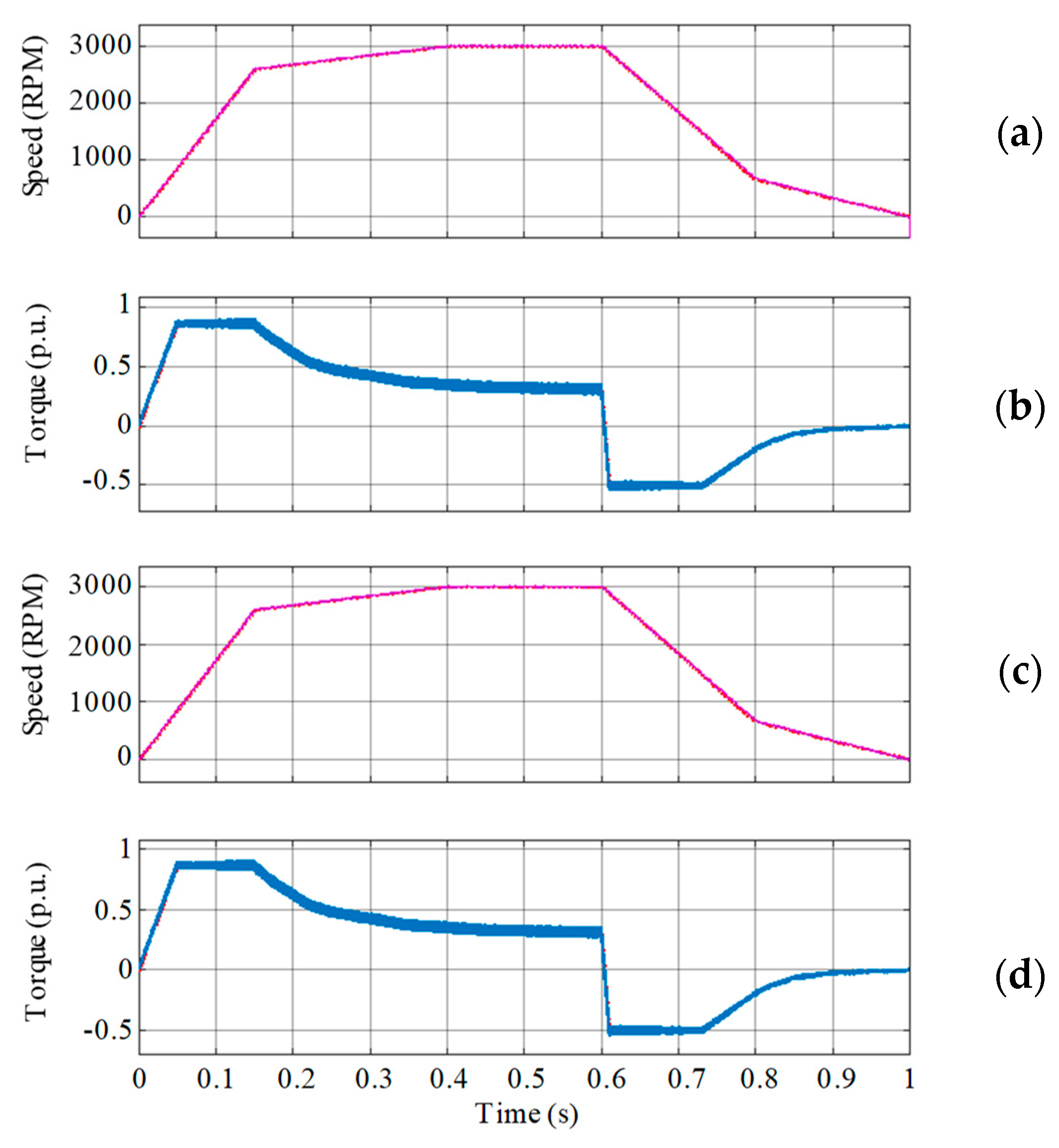
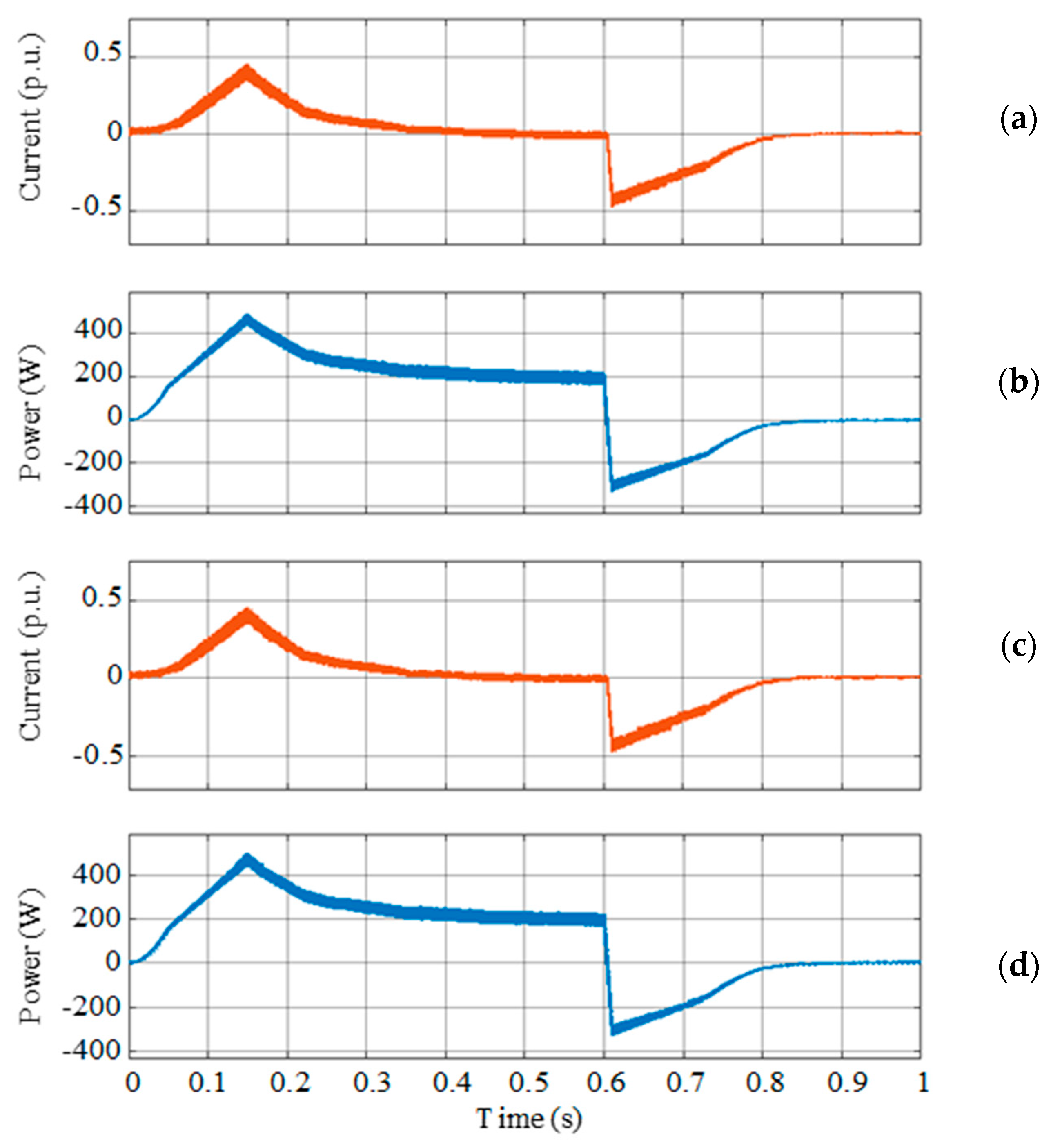
5. Simulation Studies

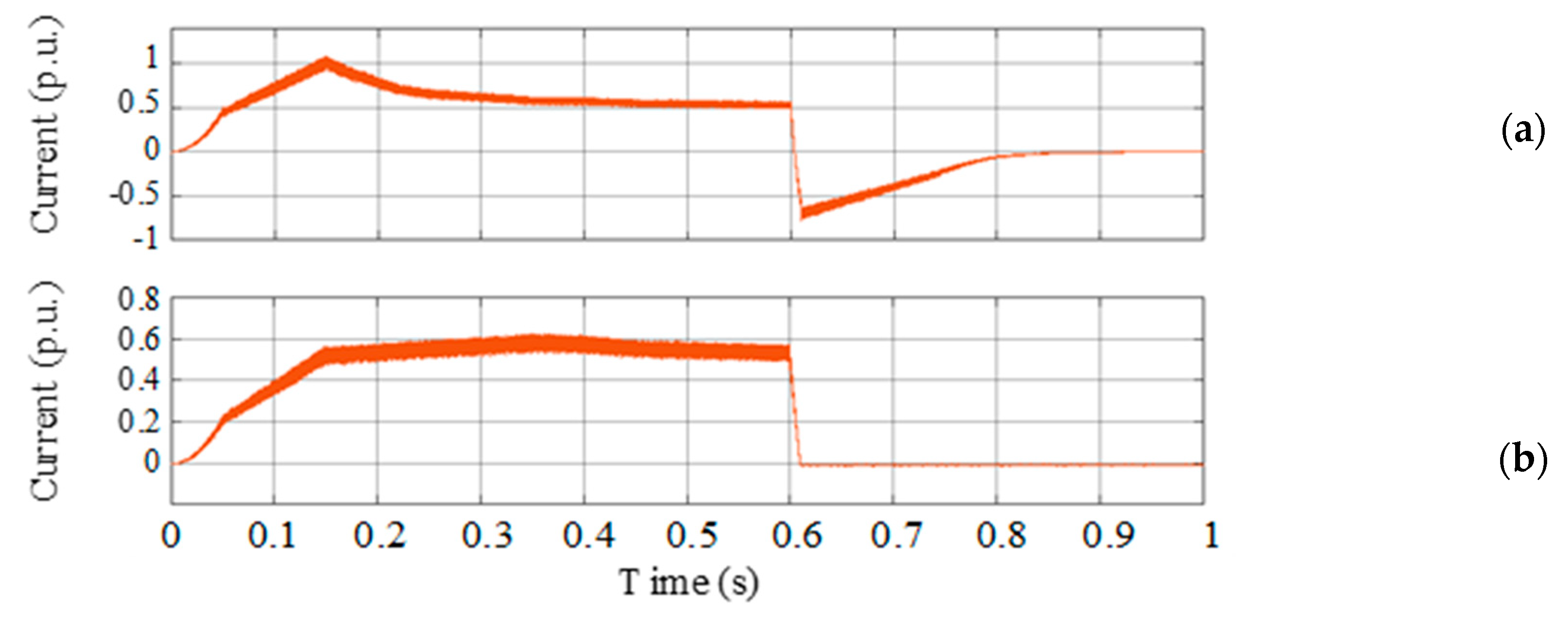
5.1. Proposed MMD Topology Validation

To demonstrate the capability of the planned MMD topology, the circuit models for both traction PMSMs and power electronic converters of the MMD were implemented in the PLECS software. Then, both the suggested model predictive control and the energy management strategy are realized in MATLAB/Simulink software to separate the models used for the controller from the models used for the propulsion system in the PLECS software environment. Therefore, the mathematical models used in the control unit are different from the circuit models that also have additional nonlinearities and non-idealities, under the verification tests. The capacity of each SC has been set to 0.33 F, with regard to PMSMs used in the test set-up. The specifications of both simulated PMSMs are acquired from the “XML-SB04A series” datasheet for the PM motors of the LS Company, the ones that are used in the experimental set-up. These specifications are reported in

Table 1. The specifications of PMSMs ¹ used in the simulation studies and the experimental set-up.

Symbol	Machine Parameters	Value
$P_{rate}$	rated power	400 Watt
$I_{rate}$	rated current	2.89 A
$p$	number of poles	$8$
$R_s$	stator resistance in phase	0.82 $\mathsf{\Omega }$
$L_d=L_q$	stator inductances	3.66 mH
${\psi }_f$	permanent magnet magnetic flux	0.0734 wb
$N_{syn}$	rated speed	3000 RPM
$T_{rate}$	rated torque	1.27 N⋅m
$T_{max}$	maximum instantaneous torque	3.82 N⋅m
$J$	moment of inertia	321$\times {10}^{-8}$ Kg.${\mathrm{m}}^2$
$B_m$	friction coefficient	$0.6\times {10}^{-6}$ N⋅m.s

¹ These data are extracted from the “XML-SB04A series” datasheet of the LS Company.

.

The switching method of all the three converters is based on the symmetric Space Vector Modulation (SVM) switching pattern. To create the symmetry in the switching pulses, the switching vector of $V_0$ is used at the beginning and end of each switching cycle, as well as the switching vector of $V_7$ is applied in the middle of each switching pulse. The converters ratings are also chosen based on the test set-up, as shown in

Table 2. The rating of converters used in the simulation studies and the experimental set-up.

Symbol	Machine Parameters	Value
$v_{in}^{dc}$	DC side voltage	173 V
$f_{SW}$	switching frequency	5 KHz
$R_{DS\left(on\right)}$	on-mode resistance of switches	0.019 Ω

.

In both internal and external control loops, the parameter h is determined as $h=0.125\times {10}^{-3}$, and the weighting matrices are considered as follows:

$$R=\left[\begin{array}{cc}1& 0\\ 0& 1\end{array}\right],Q=\left[\begin{array}{cc}15& 0\\ 0& 85\end{array}\right],Q_f=\left[\begin{array}{cc}280& 0\\ 0& 5800\end{array}\right],$$

(27)

Additionally, it is assumed that $\mathrm{\Delta }t$ in the speed controller is 0.0118 s, and the sampling frequency for the feedback signals is 20 KHz. The typical performance of the traction machines, including torque, power and speed variations during a running cycle, are depicted in Figure 5. Each running cycle is executed for a period of ${\mathrm{t}}_{\mathrm{C}}$ in both simulation and laboratory studies of the proposed MMD system integrated with the two SCs. The duration of ${\mathrm{t}}_{\mathrm{C}}$ is considered to be 1 s in the simulations. The simulated running cycle includes the three modes of charging, voltage regulation, and discharging for the SCs, in the four traction states of acceleration, constant speed, braking, and stop.

Figure 6 demonstrates the AC side currents of the simulated MMD system during a complete running cycle. All currents are in per-unit (p.u.) values on a common base of 2.89 A. The AC side currents of each S-converters, which are equal to the currents of windings in its attached OEW-PMSM, are shown in Figure 6a,b. Besides, Figure 6c, shows the HPF converter currents when there is an angle of ${\delta }^m=1.35$ radian between the rotor positions of the two machines. Through the fast acceleration stage ($0\mathrm{s}<\mathrm{t}\le 0.15\mathrm{s}$), both PMSMs runs with nominal currents, while the peak currents of HPF converter reach 53.21% more than that values. After acceleration stages, machine currents are reduced by 40% of their nominal currents, during the state of constant speed (0.4 s < t < 0.6 s).

Afterward, at t = 0.6 s the braking stage is begun. To better observe the dynamic performance of the controller, Figure 6d shows a higher resolution of the HPF converter currents in the period of the braking stage, as well. As it can be seen, the converter currents are reversed at the start time of the braking period, and then the recycled energy can be transferred to the SCs through the system converters. To prevent current spikes in the machine windings, the intense jumps are eliminated from the reference torques. Considering the variations of speeds and torques for both PMSMs, presented in Figure 7a–d, the simulated controller is able to track the references correctly, in all predetermined situations. The measured speed and torque variations are almost the same for the two machines since their references are adjusted equal to each other during the simulated running cycle.

The instantaneous powers of the two machines, as well as the DC side currents of their connected S-converters are shown in Figure 8. Since the DC side current of each S-converter is equal to the current of its connected SC, the charging and discharging currents of the two SCs also can be observed from this figure. As can be seen, during fast acceleration and motoring states, the SCs currents are positive, which means that they are delivering supplementary energy to the drive system, resulting in a reduction of DC current magnitude from the main feeder. Afterwards, at the braking times, the SCs currents are negative as they absorb the regenerated energies. Therefore, as it is shown in Figure 9, at the start of machine acceleration, the required energy is received from the main DC feeder until the amplitude of the total required DC current reaches the predetermined limit. In this simulation study, the limitation value is set to 0.5 p.u. Then, when the total receiving DC current is required to be more than 0.5 p.u., the SCs provides the extra DC current, so that the starting current from the main power supply can be restricted to the predetermined bound. Moreover, during breaking mode, when the total DC current of the drive system is negative, the regenerative energy is recuperated to SCs through the S-converters, and it can be used in the next running cycle, during propulsion. Therefore, the main supply system only provides the required energy of the traction machines, while the SC bank reduces the active power fluctuations and delivers the requisite reactive power of the drive system.

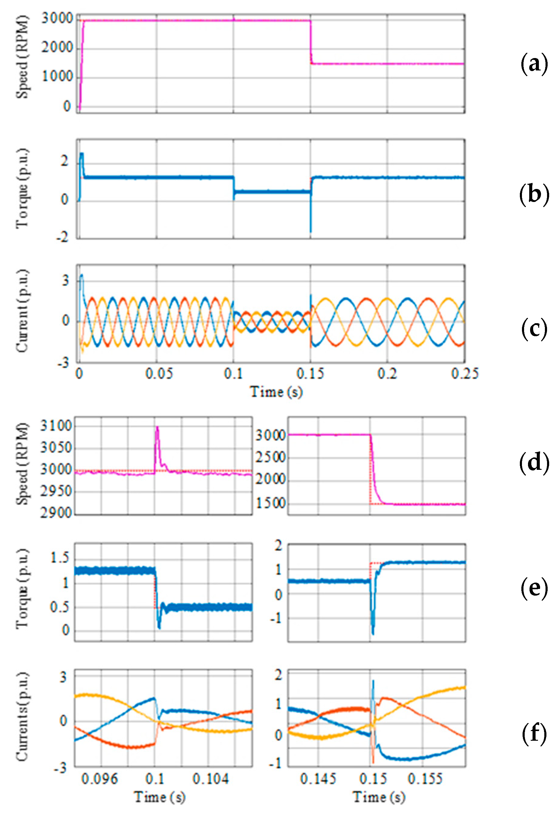
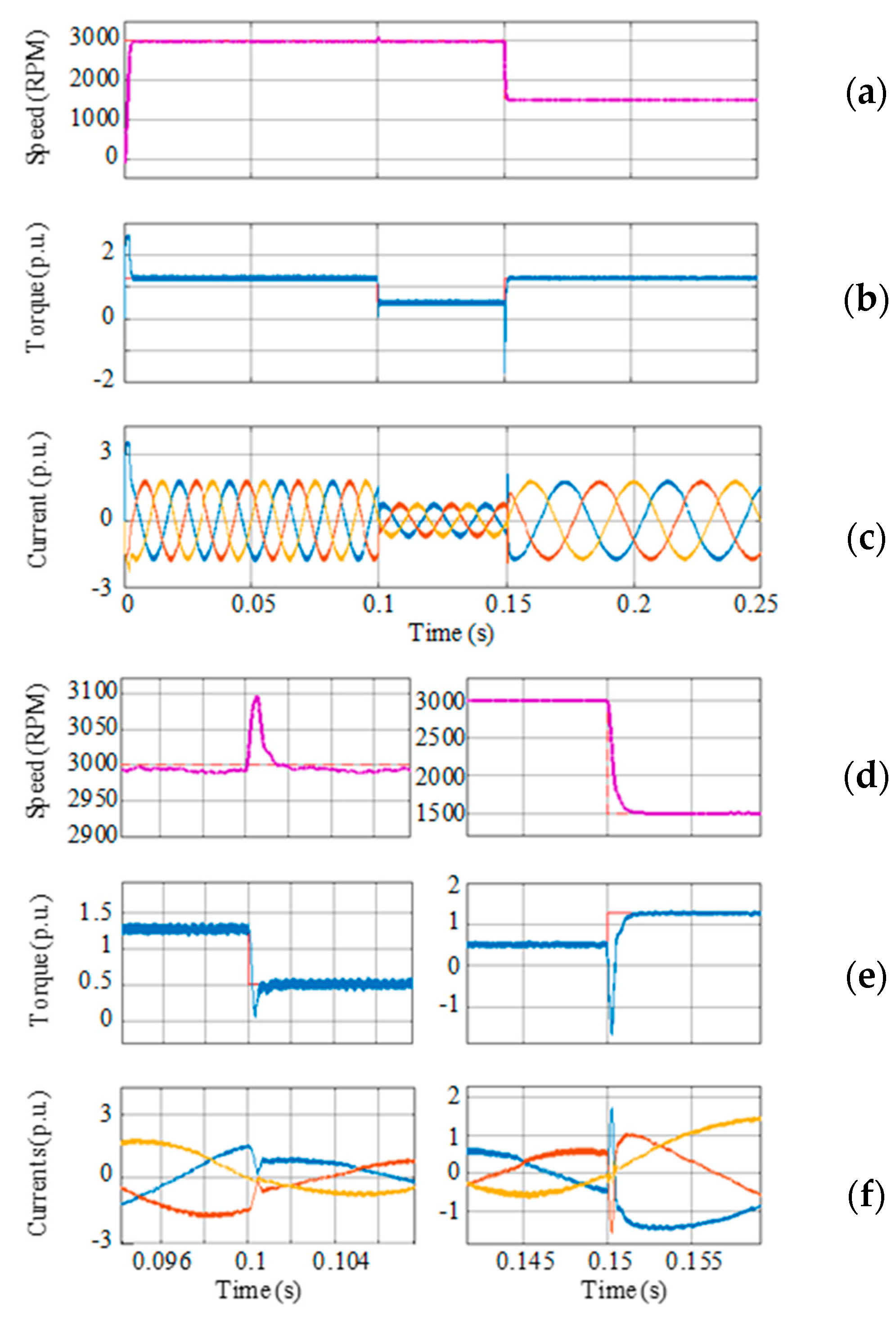
5.2. Control Dynamics Evaluation

To evaluate the validity of the designed MPC algorithm, it is compared with a simple basic MPC (SMPC) technique, in which any time limitation is not considered. In this SMPC, both amplitude and angle of voltage vectors are changed by a certain step, at each sample time, from their minimum to their maximum adequate values. After each vector shifting, the electrical equations are resolved for each PMSM and the values of the state variables including $i_q^{mx}$ are determined again. Then, for all the calculated control signals (voltage vectors), the rate of error between the calculated state variables and their reference values is evaluated by the following cost function:

$${\mathcal{J}}_{SMPC}=\underset{U_V^{mx}}{\min }\left\{K_{\psi }{\left|i_d^{mx}{}^{*}-i_d^{mx}\right|}^2+K_T{\left|i_q^{mx}{}^{*}-i_q^{mx}\right|}^2\right\}$$

(28)

Finally, the best voltage vectors ($U_V^{mx}$) is chosen based on the least error at that sample time, by calculating the cost function of (28) for all possible control signals. In order to increase the accuracy, the voltage shift step is considered to be 1% of the nominal DC voltage on the feeder side, and the angle shift step is assumed to be equal to one-tenth of a degree. Therefore, at each sampling time, the system equations together with the cost function of (28) had to be resolved 36,000 times. Although this amount of computation is very large in practice, the best possible answer for control signals can be found by using the SMPC in order to compare the results with the proposed MPC method. Nevertheless, it is supposed that, in the simulation environment, there is sufficient time to calculate and examine all those control signals in one sampling time. To investigate controller performance, the simulation results of both MPC algorithms, including speed, torque, and currents dynamics for one PMSM, are presented in Figure 10 and Figure 11. Given these figures, at first, the PMSM is loaded with its rated torque, and it is observed that the speed is increased from the stop mode to its nominal value appropriately. Then, at $\mathrm{t}=0.1\mathrm{s}$, a 70% step reduction occurred in the load torque. Besides, finally, at $\mathrm{t}=0.15\mathrm{s}$, the speed command returns to 50% of the nominal value and the load torque returns to the nominal value, concurrently and stepwise. With regard to Figure 10, by using the suggested MPC, the machine torque has reached its steady state, just five milliseconds after the start-up. Then, when the torque has a step reduction of 70% at rated speed, the output power that appears on the machine shaft could lead to severe fluctuations in the machine speed. However, by applying proposed MPC, the machine speed only increased by 100 RPM (3.333% of its rated value), and then the PMSM returns to the synchronization at the new optimal rotor angle. Moreover, the electromagnetic torque has reached the load torque at a short time, reducing undesirable machine acceleration. In this case, the controller tries to slow the speed down rapidly by moving the machine to the braking area. Meanwhile, as the speed approaches the specified reference speed, the controller does not impose any oscillating transient in the presence of increased load, and the control process is well performed by selecting the appropriate control signals at any given moment.

By comparing Figure 10 and Figure 11, it is noticed that there is almost no difference between the dynamic behaviors of SMPC and the proposed MPC, and therefore suggested MPC can track the reference trajectory with high dynamic accuracy. For a more accurate comparison between the performance of the two MPC methods, a performance index based on the integral square error (ISE) of the machine speed is defined as follows:

$$\mathrm{ISE}={\displaystyle \sum }{\left({\omega }_{ref}-{\omega }_r\right)}^2\mathrm{\Delta }t$$

(29)

Next, the ISE, as well as the harmonics index of machine currents, which is based on their total harmonics distortions (THD), are checked for the two MPC algorithms. Considering the results of these comparisons presented in

Table 3. The result comparisons between proposed MPC and SMPC, attained based on defined performance index of speed and currents THDs.

Speed	Proposed MPC	SMPC
1500 RPM	THD = 1.88	THD = 1.9
	ISE = 0.0056	ISE = 0.155
3000 RPM	THD = 1.9	THD = 1.9
	ISE = 0.0598	ISE = 0.0612

, it is perceived that the results of suggested MPC are almost the same as the SMPC at different speeds, which means that the performance and the robustness of proposed MPC are as strong as those of SMPC. Since in the SMPC, the whole vector state space is repeatedly calculated and evaluated, the required time to produce control signals is very high, whereas, the proposed method can be considered as a fast and real-time control procedure for the designed PMSMs drive system. It is also obvious that the reduction of the calculated optimal slope is perfectly proportional to the speed rate at which the machine speed approaches its nominal value. Furthermore, these simulation results show that the proposed model-based speed control can provide improved closed-loop performance as well as it can yield a fast response with small overshoots in both torque and speed tracking, simultaneously. Besides, as the suggested control laws are achieved by a simple and fast implementation, the controller has also been minimal in terms of memory allocation during simulation studies.

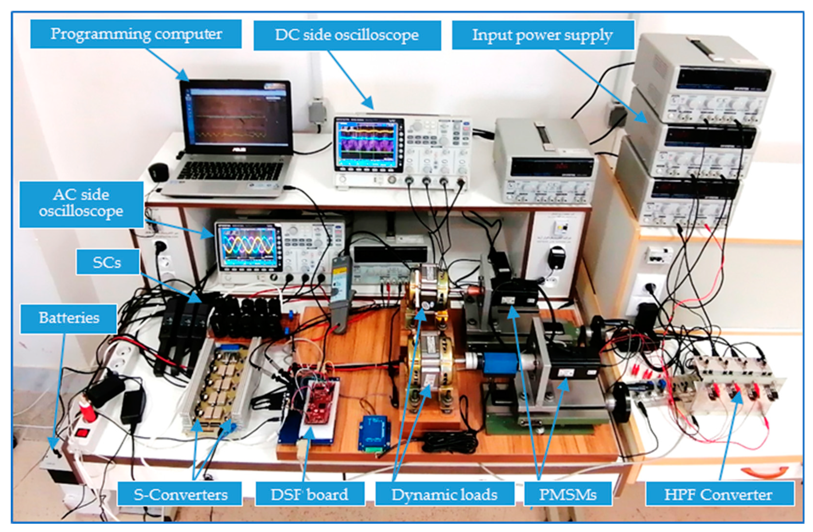
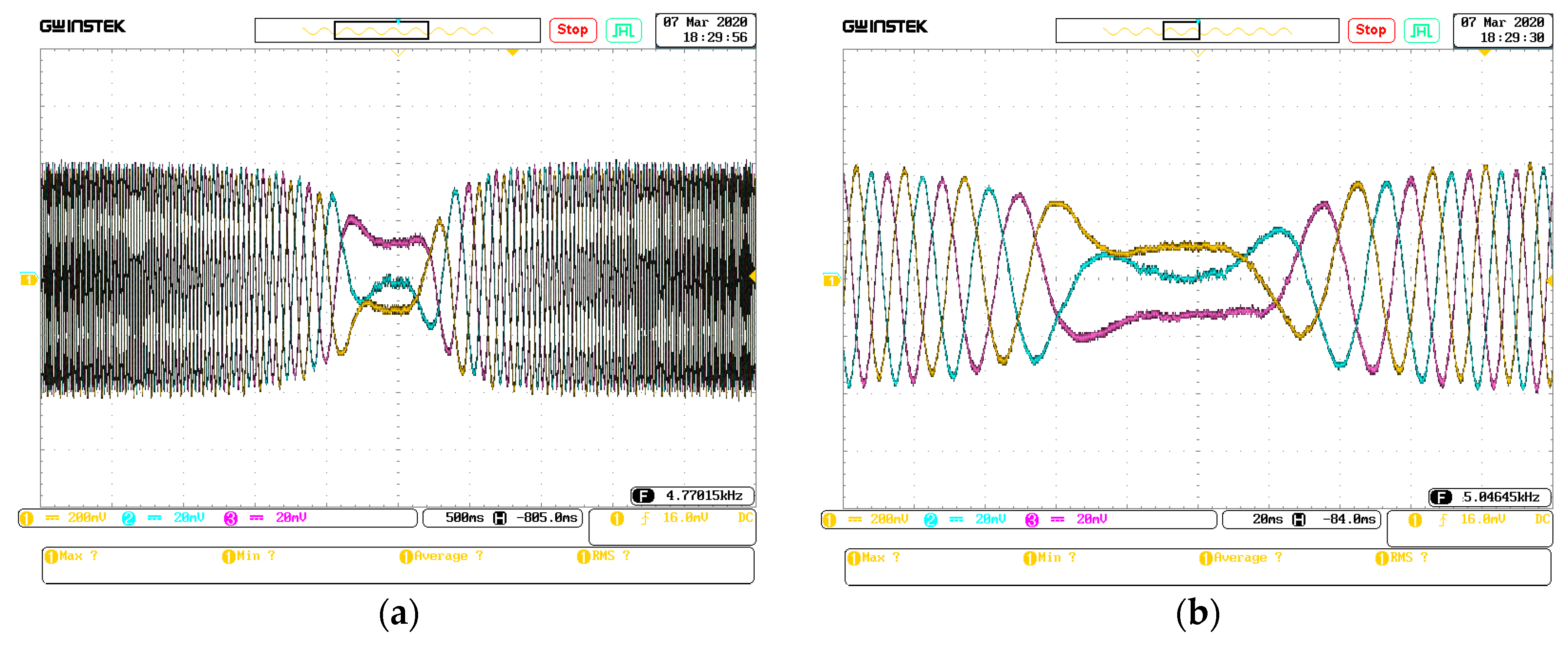
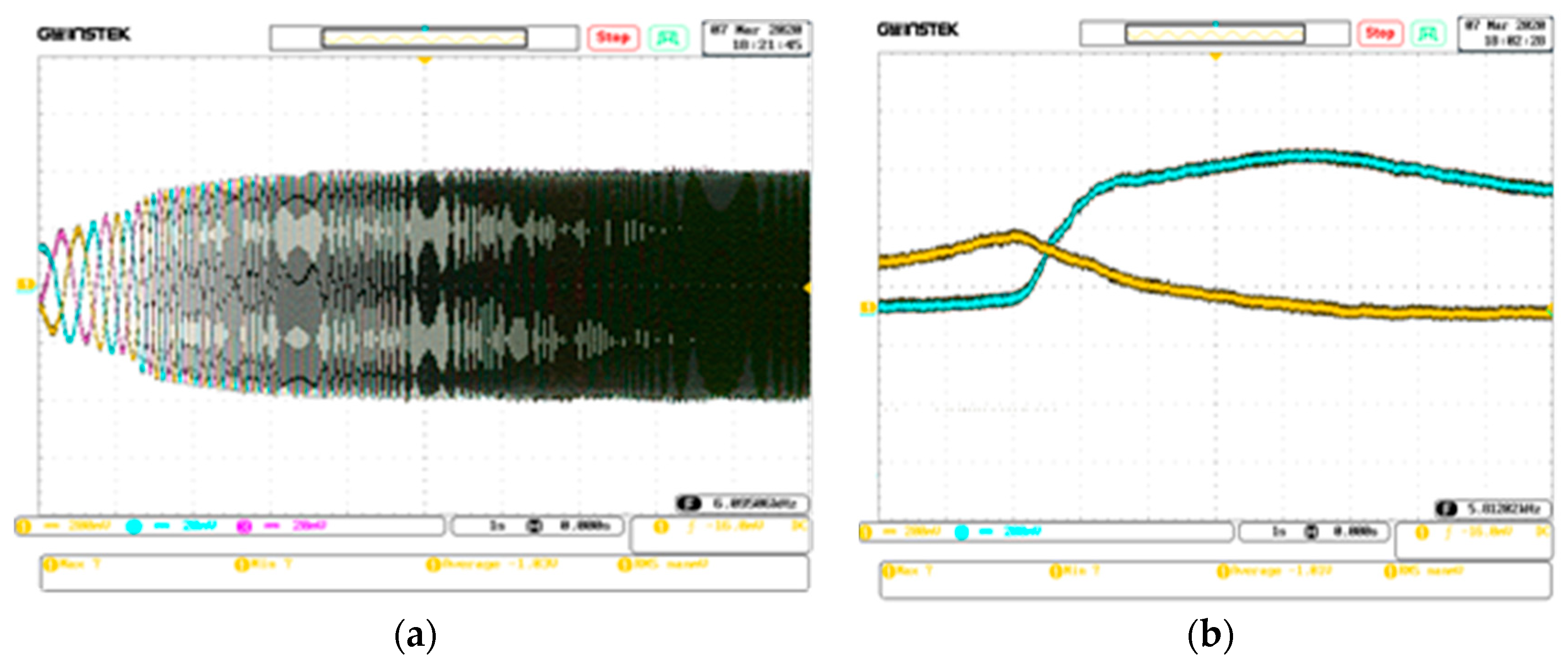
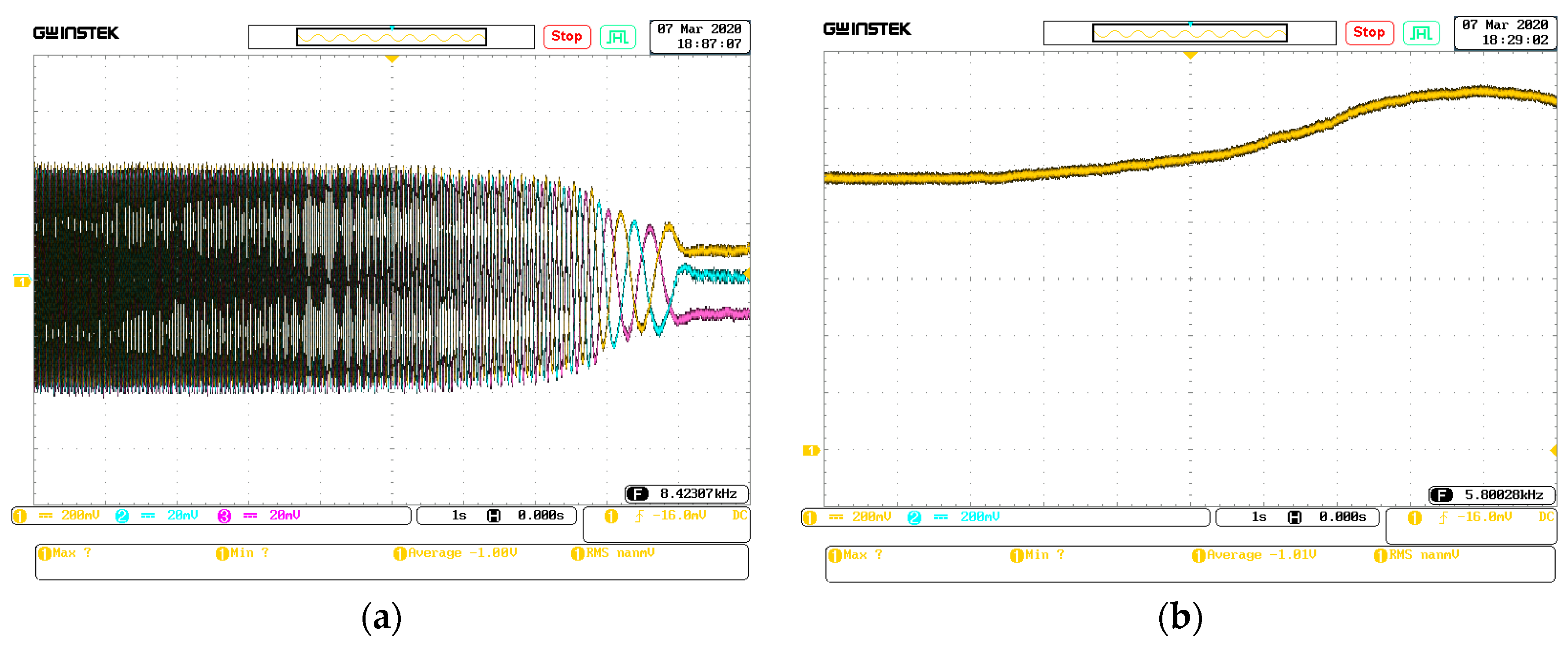
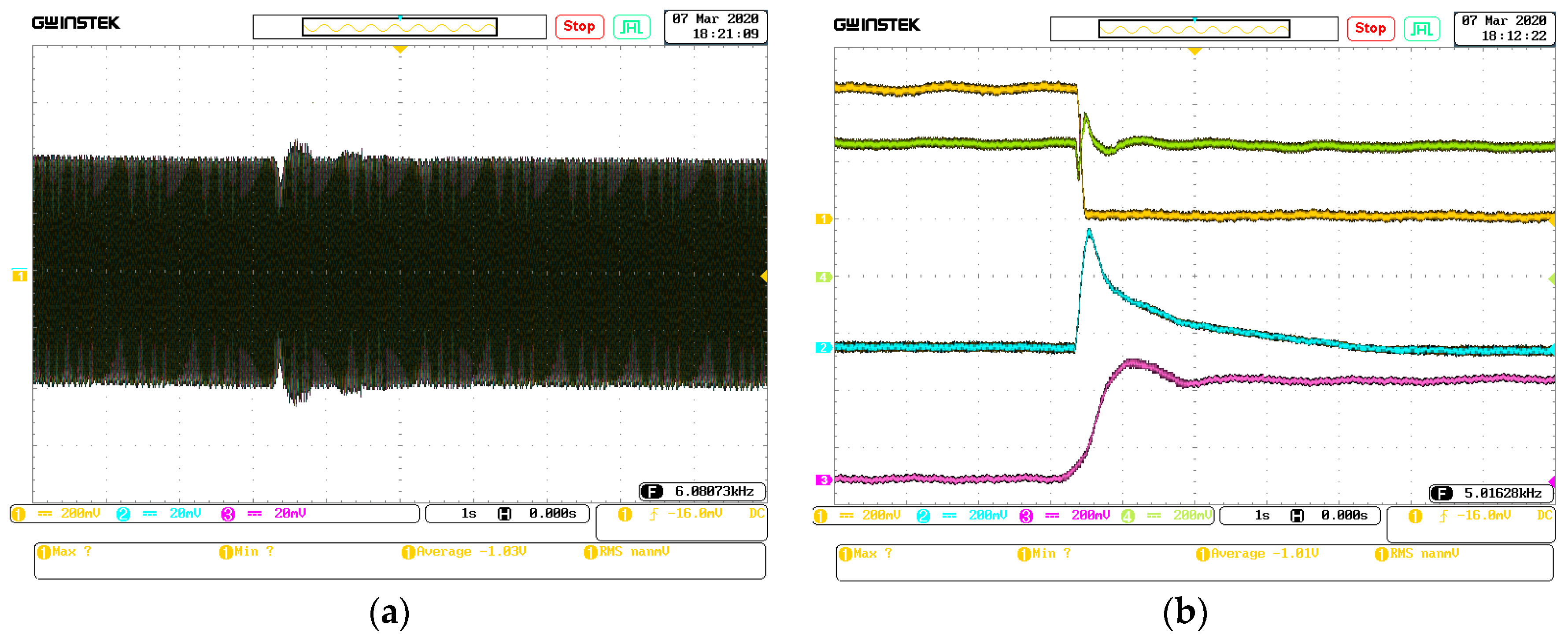
6. Experimental Setup

To evaluate the control performance of the proposed approach during the braking and acceleration transients, and to verify the power flow control and energy management strategies, a scaled prototype of the proposed hybrid ES based propulsion system was designed and manufactured, as shown in Figure 12.

The N-channel 500 V, 23 A, 245 mΩ static drain-source on resistance, 23′N50′′E power MOSFETs were used to implement the three VSI with a three-phase bridge configuration, as well as the BDC and SVR circuit boards for the prototype MMD system. Both PMSMs used in the prototype system are the PM-motors provided by the LS Company with the type of XML-SB04A, that each of them holds a self-contained encoder module. The specifications of PMSMs have been reported in Table 1. The shaft of each PMSM was also coupled to a DC generator as a controllable load, and a torque meter was used to set the machines torques manually. The electrical parameters of the set-up power circuit are presented in

Table 4. Electrical parameters of the implemented MMD.

Symbol	Parameters	Value
$v_{in}^{dc}$	input feeder voltage	173 V
$v_c^{dc}$	common DC-link voltage	170 V
$v_1^{sc}$ and $v_2^{sc}$	SCs voltage variations	90 V to 250 V
$v_t^B$	battery bank terminal voltage	85 V
$L_s^{BDC}$ and $L_s^{SVR}$	BDC and SVR inductors	1.3 m.H
$f_{SW}$	switching frequency	5 KHz

. The control algorithms, as well as the power and the energy management strategies, were uploaded on a TI LaunchXL-F28379D development kit. This DSP board facilitates communication with the programming computer, many direct connections with the analog input signals coming from the interfacing boards, and also many logical outputs to the gate’s optical isolators of the semiconductor switches.

Then, several tests were performed using this manufactured prototype system as follows:

In the first test, while both machines were rotating at the constant speed of 1000 RPM (rotations per minute) with a positive torque of 0.5 N⋅m, as the load inertia, the reference speed was changed as a step to 0 RPM, and then after stopping, it returned to the previous value of 1000 RPM, with a negative torque of 0.5 N⋅m. Figure 13a,b shows the machine’s currents during such stop and start situations. It can be observed that this process was done very quickly and smoothly without any overcurrent or severe transients since the controller was able to track the reference currents for both machines, and the current constraints were satisfied in full. Therefore, the winding voltages was distributed between the S-converters and the HPF converter sufficiently for both machines.

In the second test, the performance of the suggested MMD was assessed by the set-up system, during fast acceleration state (startup), and under the nominal load torque of the machines. Figure 14a, shows the currents of PMSM 1 in this period, and the DC side current of its connected S-converter is also depicted as beige color in Figure 14b. It can be seen that, at first, the feeder current was almost zero and the SC bank delivered the required energy to the drive system. Then, after the initial starting transients, the main feeder current increased slowly and the SCs current reduced. Note that this figure only represents the current of one S-converter and the equivalent DC current of SC bank is twice this current. Therefore, the starting current from the input feeder was limited in the fast acceleration period.

In the third test, the process of absorbing the regenerated energy at braking times was investigated. Both machine currents and the SC bank voltage of PMSM 1 can be seen in Figure 15a,b, for this duration. It can be observed that since the regenerative energy was recuperated to SCs through its connected S-converters, the DC voltage of this SC bank increased relative to the machine currents reduction.

The final test presented in this section is for evaluating the UPS functionality of the proposed propulsion systems, as the results are shown in Figure 16b. After the input power outage, the currents of both machines had some transient, although under 10% in worst-case conditions. Moreover, the voltage of common DC-link had also such a transient, however, in a very short period of time within one second at the full load, as can be seen in 16 a. The SCs aid in this duration caused an effective action, which resulted in the reduction of this transient time and the voltage variation in the common DC link.

7. Conclusions

This research provided a new railway propulsion system with uninterruptible power supply functionality, which employs hybrid energy storage to ensure the safety of train traffic and stable power supplying of onboard emergency equipment. The proposed approach can also eliminate the power fluctuations in the onboard electric power systems during different operating conditions, as it is essential for the reliable and continuous functioning of the electrified railway tractions. Besides, an innovative multi-motor drive topology has been suggested that can be considered as an effective solution for reducing peak current of the main DC supply, and decreasing voltage fluctuations of supplying DC bus, on feeder side of the electrified train, in accelerating and braking regimes. Although this topology needs added space and investment for the additional installation, it allows avoiding high economic and social costs of unpredicted service interruptions and promotes environmental sustainability by improving energy efficiency. In addition to the circuit structure, a new model-based optimal control has been developed and implemented on the proposed drive system. The designed MPC based controller is constrained, and the control signals are obtained as linear functions from the feedback states. Mathematical analyses, as well as simulation and experimental studies, have been presented, and the results show that the computation time of proposed MPC has been significantly reduced, providing the possibility for controlling the drive system with a low-cost microcontroller. Moreover, the outcomes of these studies verify the usability of onboard SCs, integrated with the suggested multi-motor drive system for the suggested system having two OEW-PMSMs. Since the improvement of train propulsion system by these suggestions can lead to a reduction in peak power demand, railway companies can increase the distance between the electric train power-substations, especially for future plans. Therefore, not only can the proposed traction drive restructuring improve the reliability and stability of electrified railway tractions under power system disturbances, but it can assist in the sustainable railroad developments.

References

1. Pietrzak, K.; Pietrzak, O. Environmental Effects of Electromobility in a Sustainable Urban Public Transport. Sustainability 2020, 12, 1052. [Google Scholar] [CrossRef] [Green Version]
2. Aguado, J.A.; Racero, A.J.; de la Torre, S. Optimal operation of electric railways with renewable energy and electric storage systems. IEEE Trans. Smart Grid 2016, 9, 993–1001. [Google Scholar] [CrossRef]
3. Ceraolo, M.; Lutzemberger, G.; Meli, E.; Pugi, L.; Rindi, A.; Pancari, G. Energy storage systems to exploit regenerative braking in DC railway systems: Different approaches to improve efficiency of modern high-speed trains. J. Energy Storage 2018, 16, 269–279. [Google Scholar] [CrossRef]
4. Van Dongen, L.A.; Frunt, L.; Martinetti, A. Smart Asset Management or Smart Operation Management? The Netherlands Railways Case. In Transportation Systems: Managing Performance through Advanced Maintenance Engineering, 1st ed.; Singh, S., Martinetti, A., Majumdar, A., van Dongen, L., Eds.; Springer (Asset Analytics): Singapore, 2019; pp. 113–132. [Google Scholar]
5. Martinetti, A.; Braaksma, A.J.J.; van Dongen, L.A.M. Beyond RAMS Design: Towards an Integral Asset and Process Approach. In Advances in Through-Life Engineering Services, 1st ed.; Redding, L., Roy, R., Shaw, A., Eds.; Springer International Publishing: Cham, Switzerland, 2017; pp. 417–428. [Google Scholar]
6. Haes Alhelou, H.; Hamedani-Golshan, M.E.; Njenda, T.C.; Siano, P. A Survey on Power System Blackout and Cascading Events: Research Motivations and Challenges. Energies 2019, 12, 682. [Google Scholar] [CrossRef] [Green Version]
7. Sinha, P. Architectural design and reliability analysis of a fail-operational brake-by-wire system from ISO 26262 perspectives. Reliab. Eng. Syst. Saf. 2011, 96, 1349–1359. [Google Scholar] [CrossRef]
8. Nagaura, Y.; Oishi, R.; Shimada, M.; Kaneko, T. Battery-powered drive systems: Latest technologies and outlook. Hitachi Rev. 2017, 66, 139. [Google Scholar]
9. Meishner, F.; Sauer, D.U. Wayside Energy Recovery Systems in DC Urban Railway Grids. eTransportation 2019, 1, 100001. [Google Scholar] [CrossRef]
10. Steiner, M.; Klohr, M.; Pagiela, S. Energy storage system with ultracaps on board of railway vehicles. In Proceedings of the 12th European Conference on Power Electronics and Applications, Aalborg, Denmark, 2 September 2007; pp. 1–10. [Google Scholar]
11. Mayrink, S., Jr.; Oliveira, J.G.; Dias, B.H.; Oliveira, L.W.; Ochoa, J.S.; Rosseti, G.S. Regenerative Braking for Energy Recovering in Diesel-Electric Freight Trains: A Technical and Economic Evaluation. Energies 2020, 13, 963. [Google Scholar] [CrossRef] [Green Version]
12. Radu, P.V.; Szelag, A.; Steczek, M. On-Board Energy Storage Devices with Supercapacitors for Metro Trains—Case Study Analysis of Application Effectiveness. Energies 2019, 12, 1291. [Google Scholar] [CrossRef] [Green Version]
13. Khodaparastan, M.; Mohamed, A.A.; Brandauer, W. Recuperation of regenerative braking energy in electric rail transit systems. IEEE Trans. Intell. Transp. Syst. 2019, 20, 2831–2847. [Google Scholar] [CrossRef] [Green Version]
14. Yildirim, D.; Aksit, M.H.; Yolacan, C.; Pul, T.; Ermis, C.; Aghdam, B.H.; Cadirci, I.; Ermis, M. Full-Scale Physical Simulator of All SiC Traction Motor Drive with On-Board Supercapacitor ESS for Light-Rail Public Transportation. IEEE Trans. Ind. Electron. 2019, 67, 6290–6301. [Google Scholar] [CrossRef]
15. Makdisie, C.J.; Mariam, M.F. Applied Power Electronics: Inverters, UPSs. In Handbook of Research on New Solutions and Technologies in Electrical Distribution Networks; IGI Global: Hershey, PA, USA, 2020; pp. 322–361. [Google Scholar]
16. Lee, Y.; Ha, J.I. Control method of mono-inverter dual parallel drive system with interior permanent magnet synchronous machines. IEEE Trans. Power Electron. 2015, 31, 7077–7086. [Google Scholar]
17. Bolvashenkov, I.; Herzog, H.G.; Ismagilov, F.; Vavilov, V.; Khvatskin, L.; Frenkel, I.; Lisnianski, A. Reliability and Fault Tolerance Assessment of Multi-motor Electric Drives with Multi-phase Traction Motors. In Fault-Tolerant Traction Electric Drives; Springer: Singapore, 2020; pp. 1–24. [Google Scholar]
18. Brando, G.; Piegari, L.; Spina, I. Simplified Optimum Control Method for Mono-inverter Dual Parallel PMSM Drive. IEEE Trans. Ind. Electron. 2017, 65, 3763–3771. [Google Scholar] [CrossRef]
19. Nagano, T.; Itoh, J.C. Parallel Connected Multiple Drive System using Small Auxiliary Inverter for Numbers of PMSMs. In Proceedings of the International Power Electronics Conference (IPEC), Hiroshima, Japan, 18–21 May 2014; pp. 1253–1260. [Google Scholar]
20. Yuan, X.; Zhang, C.; Zhang, S. A novel Deadbeat Predictive Current Control Scheme for OEW-PMSM Drives. IEEE Trans. Power Electron. 2019, 34, 11990–12000. [Google Scholar] [CrossRef]
21. Lee, Y.; Ha, J.I. Hybrid modulation of dual inverter for open-end permanent magnet synchronous motor. IEEE Trans. Power Electron. 2014, 30, 3286–3299. [Google Scholar] [CrossRef]
22. Attaianese, C.; D’Arpino, M.; Di Monaco, M.; Tomasso, G. Multi Inverter Electrical Drive for Double Motor Electric Vehicles. In Proceedings of the International Electric Vehicle Conference, Greenville, SC, USA, 4–8 March 2012; pp. 1–8. [Google Scholar]
23. Torrent, M.; Perat, J.I.; Jiménez, J.A. Permanent Magnet Synchronous Motor with Different Rotor Structures for Traction Motor in High Speed Trains. Energies 2018, 11, 1549. [Google Scholar] [CrossRef] [Green Version]
24. Du, M.; Tian, Y.; Wang, W.; Ouyang, Z.; Wei, K. A Novel Finite-Control-Set Model Predictive Directive Torque Control Strategy of Permanent Magnet Synchronous Motor with Extended Output. Electronics 2019, 8, 388. [Google Scholar] [CrossRef] [Green Version]
25. Zhang, Z.; Zhang, Z.; Garcia, C.; Rodríguez, J.; Huang, W.; Kennel, R. Discussion on control methods with finite-control-set concept for PMSM drives. In Proceedings of the International Electric Machines & Drives Conference (IEMDC), San Diego, CA, USA, 12–15 March 2019. [Google Scholar]
26. Vafaie, M.H. Performance Improvement of Permanent-Magnet Synchronous Motor through a New Online Predictive Controller. IEEE Trans. Energy Convers. 2019, 34, 2258–2266. [Google Scholar] [CrossRef]
27. Liu, H.; Li, S. Speed control for PMSM servo system using predictive functional control and extended state observer. IEEE Trans. Ind. Electron. 2011, 59, 1171–1183. [Google Scholar] [CrossRef]
28. Li, L.B.; Sun, H.X.; Chu, J.D.; Wang, G.L. The predictive control of PMSM based on state space. In Proceedings of the International Conference on Machine Learning and Cybernetics, Xi’an, China, 5 November 2003; Volume 2, pp. 859–862. [Google Scholar]
29. Chai, S.; Wang, L.; Rogers, E. Model predictive control of a permanent magnet synchronous motor. In Proceedings of the 37th Annual Conference of the IEEE Industrial Electronics Society (IECON), Melbourne, Australia, 7–10 November 2011; pp. 1928–1933. [Google Scholar]
30. Chai, S.; Wang, L.; Rogers, E. Model predictive control of a permanent magnet synchronous motor with experimental validation. Control Eng. Pract. 2013, 21, 1584–1593. [Google Scholar] [CrossRef]
31. Bemporad, A.; Morari, M.; Dua, V.; Pistikopoulos, E.N. The explicit linear quadratic regulator for constrained systems. Automatica 2002, 38, 3–20. [Google Scholar] [CrossRef]
32. Bolognani, S.; Bolognani, S.; Peretti, L.; Zigliotto, M. Design and implementation of model predictive control for electrical motor drives. IEEE Trans. Ind. Electron. 2008, 56, 1925–1936. [Google Scholar] [CrossRef]
33. Chai, S.; Wang, L.; Rogers, E. A cascade MPC control structure for a PMSM with speed ripple minimization. IEEE Trans. Ind. Electron. 2012, 60, 2978–2987. [Google Scholar] [CrossRef] [Green Version]
34. Tøndel, P.; Johansen, T.A.; Bemporad, A. Evaluation of piecewise affine control via binary search tree. Automatica 2003, 39, 945–950. [Google Scholar] [CrossRef] [Green Version]
35. Pirouz, H.M.; Bina, M. A transformerless medium-voltage STATCOM topology based on extended modular multilevel converters. IEEE Trans. Power Electron. 2010, 26, 1534–1545. [Google Scholar]
36. Zhan, H.; Zhu, Z.Q.; Odavic, M. Analysis and suppression of zero sequence circulating current in open winding PMSM drives with common DC bus. IEEE Trans. Ind. Appl. 2017, 53, 3609–3620. [Google Scholar] [CrossRef]
37. Di Cairano, S.; Bemporad, A. Model predictive control tuning by controller matching. IEEE Trans. Autom. Control 2009, 55, 185–190. [Google Scholar] [CrossRef]
38. Saerens, B.; Diehl, M.; Van den Bulck, E. Optimal control using Pontryagin’s maximum principle and dynamic programming. In Automotive Model Predictive Control; Springer: London, UK, 2010; pp. 119–138. [Google Scholar]
39. Xu, Y.; Shi, T.; Yan, Y.; Gu, X. Dual-Vector Predictive Torque Control of Permanent Magnet Synchronous Motors Based on a Candidate Vector Table. Energies 2019, 12, 163. [Google Scholar] [CrossRef] [Green Version]
40. Liu, K.; Zhu, Z.Q. Mechanical parameter estimation of permanent-magnet synchronous machines with aiding from estimation of rotor PM flux linkage. IEEE Trans. Ind. Appl. 2015, 51, 3115–3125. [Google Scholar] [CrossRef]
Figure 1. The circuit diagrams of prolusion systems with auxiliary onboard uninterruptible power supplies (UPS) in a railway traction bogie: (a) The diagram of a conventional traction multi-machine drive (MMD) including two induction machines (IMs) and a shared converter, (b) the diagram of proposed hybrid-ES based MMD, including two open-end winding Permanent Magnet Synchronous Machines (OEW-PMSMs) which are attached to the S-converters having supercapacitor (SC) banks in their DC-links, in addition to the SCs voltage regulator (SVR) circuit, all being replaced with the two IMs in the parallel-connected IMs based MMD system of (a). The blue areas contain the newly added power electronics and SCs, compared to the old green areas.
Sustainability 12 03943 g001
Figure 2. The proposed onboard power system supported by backup batteries, planned for an electric train and tram (ET) with two bogies, each with two traction machines.
Sustainability 12 03943 g002
Figure 3. The voltage vectors of the two machines and all converters.
Sustainability 12 03943 g003
Figure 4. The architecture of the proposed control method.
Sustainability 12 03943 g004
Figure 5. The executed running cycle for the proposed MMD: The parameters of ω T   ,   P T and T L are the speed, the power, and the total torque of the traction system, respectively. E T also is the value of energy demand of the two PM machines and the MMD converters in the traction system. Besides, the period of charging, voltage regulation, and discharging times for the SCs are added.
Sustainability 12 03943 g005
Figure 6. Simulation results: (a) The three-phase currents of the first PMSM that are equal to the AC side currents of the first S-converters, (b) the three-phase currents of the second PMSM that are equal to the AC side currents of the second S-converters, (c) the total currents both PMSMs that are equal to the AC side currents of the HPF converter, (d) a closer look at the total PMSMs currents during transients. All currents are shown in per-unit (p.u.) and the base value is 2.89 A (its rated value) reduced by 40% of their nominal currents, during the state of constant speed ( 0.4   s < t < 0.6   s ). Afterward, at t = 0.6   s the braking stage is begun.
Sustainability 12 03943 g006
Figure 7. Simulation results: (a) and (b) the speed and the torque profiles respectively for PMSM 1, (c) and (d) The speed and the torque profiles respectively for PMSM 2. Speeds are measured in rotations per minute (RPM), and torque is measured in p.u. value on a base of 1.27 N⋅m (its rated value). The red dotted lines represent the reference values.
Sustainability 12 03943 g007
Figure 8. Simulation results: (a) and (b) the DC side currents of S-converters of 1 and 2, respectively, that are equal to the currents of their SCs, all in p.u., (c) and (d) the instantaneous powers of PMSMs 1 and 2, respectively.
Sustainability 12 03943 g008
Figure 9. Simulation results. Total DC current from the input feeder: (a) When the SC bank is removed, (b) when the SCs are connected to the S-converters.
Sustainability 12 03943 g009
Figure 10. Simulation results. The parameters of simulated PMSM controlled by the proposed MPC, during a 0.25 s course: (a) The speed, (b) the torque, (c) three phase currents of windings. In addition, parameters variations when the reference signals have shift steps in their values, at t = 0.1 and t = 0.15 s: (d) The speed variations, (e) the torque variations, (f) the currents variations. In this figure, all red dotted lines are the reference signals.
Sustainability 12 03943 g010
Figure 11. Simulation results. The parameters of simulated PMSM controlled by the SMPC, during a 0.25 s course: (a) The speed, (b) the torque, (c) three phase currents of windings. In addition, parameters variations when the reference signals have shift steps in their values, at t = 0.1 and t = 0.15 s: (d) The speed variations, (e) the torque variations, (f) the currents variations. In this figure, all red dotted lines are the reference signals.
Sustainability 12 03943 g011
Figure 12. The picture of manufactured experimental setup for verifying proposed system topology.
Sustainability 12 03943 g012
Figure 13. Experimental results. The dynamic performance of the current controller, during machine stop and start: (a) The currents of PMSM 1, (b) the currents of PMSM2, with higher resolutions.
Sustainability 12 03943 g013
Figure 14. Experimental results. The start-up process of the traction machines with the aid of SCs: (a) The currents of PMSM1, (b) currents of the main feeder (channel 2—the cyan color) and one of SCs (channel 1—the beige color).
Sustainability 12 03943 g014
Figure 15. Experimental results. The stop process of the traction machines with the aid of SCs: (a) Currents of PMSM1, (b) voltage of the SCs during the regenerative braking state.
Sustainability 12 03943 g015
Figure 16. Experimental results. The investigation of UPS function of the prototype system under the voltage outage condition in the input feeder: (a) Currents of PMSM1, (b) voltages of the common DC link (channel 4—the green color) and input feeder (channel 1—the beige color), as well as currents of SC bank 1 (channel 2—the cyan color) and battery bank (channel 3—the purple color).
Sustainability 12 03943 g016