Measurement of Systemic Risk in Global Financial Markets and Its Application in Forecasting Trading Decisions


 and
and
Abstract
:1. Introduction
2. Methodology
2.1. Model for Marginals
2.2. Factor Copula Models
2.3. Component Expected Shortfall
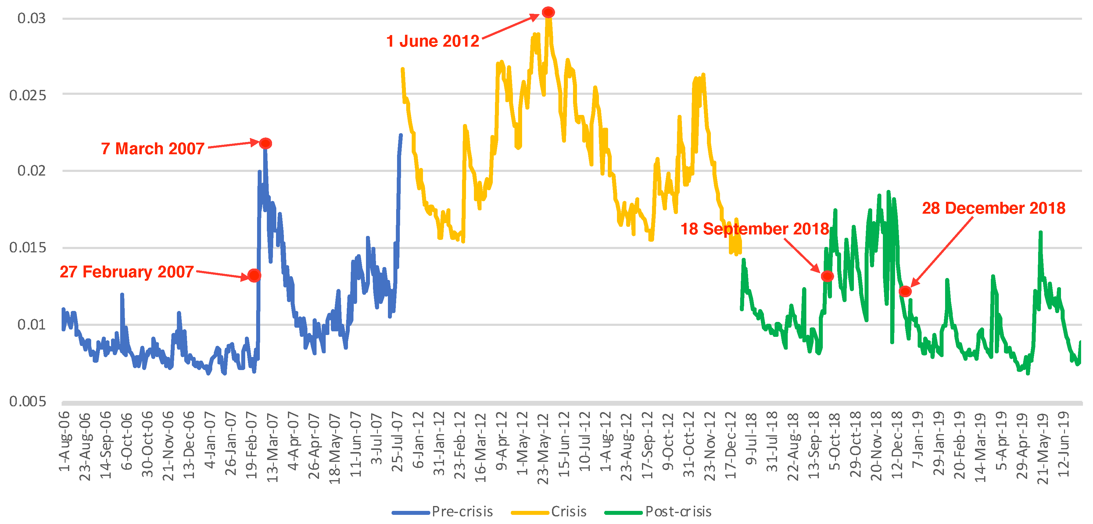
3. The Data
4. Empirical Results
4.1. Estimation Results for Factor Copula
4.2. Estimation Results for CES
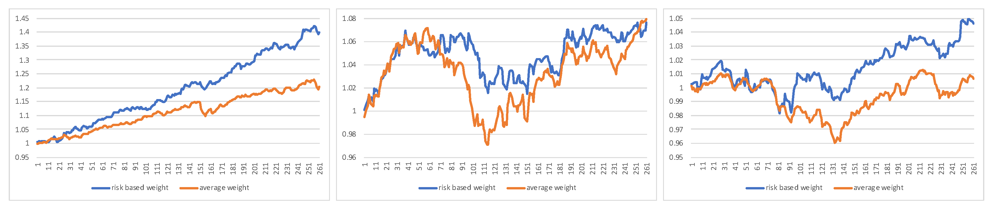
4.3. Computing Portfolios CES
- 1
- Calculate the partial derivatives of to get marginal ES(MES).
- 2
- Sort the in descending order and the MES in ascending order.
- 3
- Allocate the ith ranking country in MES with the ith ranking weight in .
5. Conclusions
Author Contributions
Funding
Acknowledgments
Conflicts of Interest
References
- Gong, C.; Tang, P.; Wang, Y. Measuring the network connectedness of global stock markets. Phys. Stat. Mech. Appl. 2019, 535, 122351. [Google Scholar] [CrossRef]
- Peters, B.G.; Pierre, J.; Randma-Liiv, T. Global financial crisis, public administration and governance: Do new problems require new solutions? Public Organ. Rev. 2011, 11, 13–27. [Google Scholar] [CrossRef]
- Arnold, P.J. Global financial crisis: The challenge to accounting research. Account. Organ. Soc. 2009, 34, 803–809. [Google Scholar] [CrossRef]
- Li, B.; Wang, T.; Tian, W. Risk measures and asset pricing models with new versions of Wang transform. In Uncertainty Analysis in Econometrics with Applications; Springer: Berlin/Heidelberg, Germany, 2013; pp. 155–167. [Google Scholar]
- Oh, D.H.; Patton, A.J. Time-varying systemic risk: Evidence from a dynamic copula model of cds spreads. J. Bus. Econ. Stat. 2018, 36, 181–195. [Google Scholar] [CrossRef] [Green Version]
- Bartram, S.M.; Brown, G.W.; Hund, J.E. Estimating systemic risk in the international financial system. J. Financ. Econ. 2007, 86, 835–869. [Google Scholar] [CrossRef] [Green Version]
- Song, Q.; Liu, J.; Sriboonchitta, S. Risk Measurement of Stock Markets in BRICS, G7, and G20: Vine Copulas versus Factor Copulas. Mathematics 2019, 7, 274. [Google Scholar] [CrossRef] [Green Version]
- Richardson, M.; Philippon, T.; Pedersen, L.H.; Acharya, V.V. Measuring Systemic Risk (No. 1002); Federal Reserve Bank of Cleveland: Cleveland, OH, USA, 2010. [Google Scholar]
- Brownlees, C.; Robert, E. Volatility, Correlation and Tails for Systemic Risk Measurement; Working paper; New York University Stern School of Business: New York, NY, USA, 2011. [Google Scholar]
- Banulescu, G.D.; Dumitrescu, E.I. Which are the SIFIs? A Component Expected Shortfall approach to systemic risk. J. Bank. Financ. 2015, 50, 575–588. [Google Scholar] [CrossRef]
- Reboredo, J.C.; Ugolini, A. A vine-copula conditional value-at-risk approach to systemic sovereign debt risk for the financial sector. N. Am. J. Econ. Financ. 2015, 32, 98–123. [Google Scholar] [CrossRef]
- Bartels, M.; Ziegelmann, F.A. Market risk forecasting for high dimensional portfolios via factor copulas with GAS dynamics. Insur. Math. Econ. 2016, 70, 66–79. [Google Scholar] [CrossRef]
- Shahzad, S.J.H.; Arreola-Hernandez, J.; Bekiros, S.; Shahbaz, M.; Kayani, G.M. A systemic risk analysis of Islamic equity markets using vine copula and delta CoVaR modeling. J. Int. Financ. Mark. Inst. Money 2018, 56, 104–127. [Google Scholar] [CrossRef]
- Yang, L.; Ma, J.Z.; Hamori, S. Dependence structures and systemic risk of government securities markets in central and eastern europe: A CoVaR-Copula approach. Sustainability 2018, 10, 324. [Google Scholar] [CrossRef] [Green Version]
- Zhang, X.; Wei, C.; Zedda, S. Analysis of China Commercial Banks’ Systemic Risk Sustainability through the Leave-One-Out Approach. Sustainability 2020, 12, 203. [Google Scholar] [CrossRef] [Green Version]
- Wu, C.C.; Chung, H.; Chang, Y.H. The economic value of co-movement between oil price and exchange rate using copula-based GARCH models. Energy Econ. 2012, 34, 270–282. [Google Scholar] [CrossRef]
- Yun, J.; Moon, H. Measuring systemic risk in the Korean banking sector via dynamic conditional correlation models. Pac.-Basin Financ. J. 2014, 27, 94–114. [Google Scholar] [CrossRef] [Green Version]
- Calabrese, R.; Osmetti, S.A. A new approach to measure systemic risk: A bivariate copula model for dependent censored data. Eur. J. Oper. Res. 2019, 279, 1053–1064. [Google Scholar] [CrossRef]
- Wei, Z.; Kim, S.; Choi, B.; Kim, D. Multivariate Skew Normal Copula for Asymmetric Dependence: Estimation and Application. Int. J. Inf. Technol. Decis. Mak. 2019, 18, 365–387. [Google Scholar] [CrossRef]
- Liu, J.; Wang, M.; Sriboonchitta, S. Examining the Interdependence between the Exchange Rates of China and ASEAN Countries: A Canonical Vine Copula Approach. Sustainability 2019, 11, 5487. [Google Scholar] [CrossRef] [Green Version]
- Reboredo, J.C.; Ugolini, A. Systemic risk in European sovereign debt markets: A CoVaR-copula approach. J. Int. Money Financ. 2015, 51, 214–244. [Google Scholar] [CrossRef]
- Pourkhanali, A.; Kim, J.M.; Tafakori, L.; Fard, F.A. Measuring systemic risk using vine-copula. Econ. Model. 2016, 53, 63–74. [Google Scholar] [CrossRef]
- Oh, D.H.; Patton, A.J. Modeling dependence in high dimensions with factor copulas. J. Bus. Econ. Stat. 2017, 35, 139–154. [Google Scholar] [CrossRef]
- Krupskii, P.; Joe, H. Factor copula models for multivariate data. J. Multivar. Anal. 2013, 120, 85–101. [Google Scholar] [CrossRef]
- Acharya, V.; Engle, R.; Richardson, M. Capital shortfall: A new approach to ranking and regulating systemic risks. Am. Econ. Rev. 2012, 102, 59–64. [Google Scholar] [CrossRef] [Green Version]
- Tiwari, A.K.; Trabelsi, N.; Alqahtani, F.; Raheem, I.D. Systemic risk spillovers between crude oil and stock index returns of G7 economies: Conditional value-at-risk and marginal expected shortfall approaches. Energy Econ. 2020, 104646. [Google Scholar] [CrossRef]
- Kleinow, J.; Moreira, F.; Strobl, S.; Vähämaa, S. Measuring systemic risk: A comparison of alternative market-based approaches. Financ. Res. Lett. 2017, 21, 40–46. [Google Scholar] [CrossRef]
- Benoit, S.; Colletaz, G.; Hurlin, C.; Pérignon, C. A theoretical and empirical comparison of systemic risk measures. SSRN Electron. J. 2013. [Google Scholar] [CrossRef]
- Adrian, T.; Brunnermeier, M.K. CoVaR (No. w17454); National Bureau of Economic Research: Cambridge, MA, USA, 2011. [Google Scholar]
- Reboredo, J.C. Is there dependence and systemic risk between oil and renewable energy stock prices? Energy Econ. 2015, 48, 32–45. [Google Scholar] [CrossRef]
- Reboredo, J.C.; Rivera-Castro, M.A.; Ugolini, A. Downside and upside risk spillovers between exchange rates and stock prices. J. Bank. Financ. 2016, 62, 76–96. [Google Scholar] [CrossRef]
- Liu, J.; Sriboonchitta, S.; Phochanachan, P.; Tang, J. Volatility and dependence for systemic risk measurement of the international financial system. In Proceedings of the International Symposium on Integrated Uncertainty in Knowledge Modelling and Decision Making, Nha Trang, Vietnam, 15–17 October 2015; Springer: Cham, Switzerland, 2015; pp. 403–414. [Google Scholar]
- Wu, F. Sectoral contributions to systemic risk in the Chinese stock market. Financ. Res. Lett. 2019, 31. [Google Scholar] [CrossRef]
- Du, L.; He, Y. Extreme risk spillovers between crude oil and stock markets. Energy Econ. 2015, 51, 455–465. [Google Scholar] [CrossRef]
- Silvapulle, P.; Smyth, R.; Zhang, X.; Fenech, J.P. Nonparametric panel data model for crude oil and stock market prices in net oil importing countries. Energy Econ. 2017, 67, 255–267. [Google Scholar] [CrossRef]
- Matesanz, D.; Ortega, G.J. Sovereign public debt crisis in Europe. A network analysis. Phys. Stat. Mech. Appl. 2015, 436, 756–766. [Google Scholar] [CrossRef]
- Bauer, G.H.; Granziera, E. Monetary policy, private debt and financial stability risks. Int. J. Cent. Bank. 2016, 13, 337–373. [Google Scholar] [CrossRef] [Green Version]
- Equiza-Goñi, J. Government debt maturity and debt dynamics in euro area countries. J. Macroecon. 2016, 49, 292–311. [Google Scholar] [CrossRef]
- Glosten, L.R.; Jagannathan, R.; Runkle, D.E. On the relation between the expected value and the volatility of the nominal excess return on stocks. J. Financ. 1993, 48, 1779–1801. [Google Scholar] [CrossRef]
- Warshaw, E. Extreme dependence and risk spillovers across north american equity markets. N. Am. J. Econ. Financ. 2019, 47, 237–251. [Google Scholar] [CrossRef]
- Christensen, B.J.; Nielsen, M.Ø.; Zhu, J. The impact of financial crises on the risk–return tradeoff and the leverage effect. Econ. Model. 2015, 49, 407–418. [Google Scholar] [CrossRef] [Green Version]
- Stroud, A.H.; Secrest, D. Gaussian Quadrature Formulas. 1966. Available online: https://cds.cern.ch/record/104292 (accessed on 13 May 2020).
- Basel Committee on Banking Supervision. Minimum Capital Requirements for Market Risk; Basel Committee on Banking Supervision: Basel, Switzerland, 2016. [Google Scholar]
- Stoyanov, S.V.; Racheva-Iotova, B.; Rachev, S.T.; Fabozzi, F.J. Stochastic models for risk estimation in volatile markets: A survey. Ann. Oper. Res. 2010, 176, 293–309. [Google Scholar] [CrossRef]
- Rachev, S.T.; Stoyanov, S.V.; Fabozzi, F.J. Advanced Stochastic Models, Risk Assessment, and Portfolio Optimization: The Ideal Risk, Uncertainty, and Performance Measures; Wiley: New York, NY, USA, 2008; Volume 149. [Google Scholar]
- Ghalanos, A. Package ‘rugarch’; R Team Cooperation: Seattle, WA, USA, 2018. [Google Scholar]
- Joe, H. Dependence Modeling with Copulas; CRC Press: Boca Raton, FL, USA, 2014. [Google Scholar]
- Peterson, B.G.; Carl, P.; Boudt, K.; Bennett, R.; Ulrich, J.; Zivot, E.; Cornilly, D.; Hung, E.; Lestel, M.; Balkissoon, K. Package ‘PerformanceAnalytics’. 2015. Available online: https://CRAN.R-project.org/package=PerformanceAnalytics (accessed on 18 October 2018).
- Tachibana, M. Relationship between stock and currency markets conditional on the US stock returns: A vine copula approach. J. Multinatl. Financ. Manag. 2018, 46, 75–106. [Google Scholar] [CrossRef] [Green Version]
- Allen, D.; McAleer, M.; Singh, A. Risk measurement and risk modelling using applications of vine copulas. Sustainability 2017, 9, 1762. [Google Scholar] [CrossRef] [Green Version]
- Hatzius, J.; Stehn, J. The US Economy in 2013–2016: Moving Over the Hump; Goldman Sachs: New York, NY, USA, 2012. [Google Scholar]
- Schwab, K. World Economic Forum, Global Competitiveness Report (2012–2013); World Economic Forum: Geneva, Switzerland, 2012. [Google Scholar]
- Grech, A.G.; Micallef, B.; Zerafa, S.; Gauci, T.M. The Central Bank of Malta’s First Fifty Years: A Solid Foundation for the Future; Central Bank of Malta: Valletta, Malta, 2018. [Google Scholar]
- Qin, X.; Zhou, C. Financial structure and determinants of systemic risk contribution. Pac.-Basin Financ. J. 2019, 57, 101083. [Google Scholar] [CrossRef]
- Qin, X.; Zhu, X. Too non-traditional to fail? Determinants of systemic risk for BRICs banks. Appl. Econ. Lett. 2014, 21, 261–264. [Google Scholar] [CrossRef]
- Sedunov, J. What is the systemic risk exposure of financial institutions? J. Financ. Stab. 2016, 24, 71–87. [Google Scholar] [CrossRef]


| Country | Name | Country | Name | Country | Name |
|---|---|---|---|---|---|
| United States | SPX | India | SENSEX | Hungary | BUX |
| England | UXK | Saudi | TASI | Ireland | ISEQ |
| Japan | NI225 | South Africa | JTOPI | Latvia | OMXRGI |
| France | CAC40 | Turkey | XU100 | Lithuania | OMXVGI |
| Germany | DAX30 | Austria | ATX | Luxembourg | LUXX |
| Canada | SandP/TSX | Belgium | BEL20 | Malta | MSE |
| Italy | FTSEMIB | Bulgaria | SOFIX | Netherlands | AEX |
| Russian | IMOEX | Cyprus | CYMAIN | Poland | WIG20 |
| Australia | SandP/ASX20 | Croatia | CRBEX | Portugal | PSI20 |
| China | SHCOMP | Czech Republic | PX | Romania | BETI |
| Brazil | IBOVESPA | Denmark | OMXC20 | Slovakia | SAX |
| Argentina | MERVAL | Estonia | OMXTGI | Slovenia | SBITOP |
| Mexico | SandP/BMV | Finland | OMXH25 | Spain | IBEX |
| Korea | KOSPI | Greece | ATG | Sweden | OMXS30 |
| Indonesia | JKSE |
| Period | Gaussian | Frank | t-Copula | Gumbel | |
|---|---|---|---|---|---|
| pre | AIC | −4001.889 | −5219.750 | −5066.657 | −5724.441 |
| BIC | −4158.405 | −5376.265 | −5223.172 | −5880.956 | |
| in | AIC | −27,238.640 | −30,307.380 | −28,853.510 | −28,674.900 |
| BIC | −27,410.311 | −30,472.891 | −29,025.182 | −28,853.515 | |
| post | AIC | −19,457.490 | −22,915.350 | −21,266.656 | −21,498.255 |
| BIC | −19,632.780 | −23,090.630 | −21,441.930 | −21,673.532 |
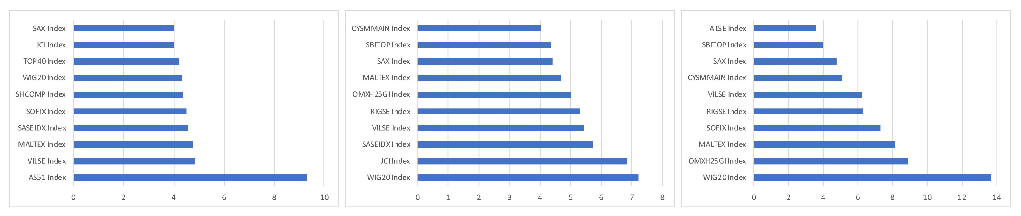
| Pre-Crisis (Gumbel) | Crisis (Frank) | Post-Crisis (Frank) | |||||||||
|---|---|---|---|---|---|---|---|---|---|---|---|
| Top 10 | Last 10 | Top 10 | Last 10 | Top 10 | Last 10 | ||||||
| Slovakia | 2.863 *** | Bulgaria | 1.036 *** | France | 4.997 *** | Lithuania | 1.268 *** | France | 3.369 *** | Lithuania | 1.126 *** |
| Netherlands | 2.775 *** | Australia | 1.033 *** | Netherlands | 4.364 *** | Japan | 1.239 *** | Netherlands | 3.092 *** | Slovenia | 1.125 *** |
| Sweden | 2.732 *** | France | 1.029 *** | Germany | 3.984 *** | Bulgaria | 1.188 *** | Germany | 2.969 *** | China | 1.122 *** |
| Spain | 2.498 *** | England | 1.028 *** | England | 3.678 *** | Slovenia | 1.146 *** | Belgium | 2.934 *** | Croatia | 1.121 *** |
| Belgium | 2.345 *** | Saudi | 1.026 *** | Italy | 3.466 *** | Saudi | 1.142 *** | Slovakia | 2.745 *** | Cyprus | 1.086 *** |
| Ireland | 1.769 *** | China | 1.020 *** | Belgium | 3.375 *** | China | 1.127 ** | Sweden | 2.685 *** | Latvia | 1.081 *** |
| Denmark | 1.740 *** | Poland | 1.016 *** | Slovakia | 3.218 *** | Latvia | 1.098 *** | Spain | 2.616 *** | Bulgaria | 1.058 *** |
| Austria | 1.669 *** | Latvia | 1.014 *** | Spain | 3.071 *** | Finland | 1.023 *** | Italy | 2.501 *** | Finland | 1.019 *** |
| Portugal | 1.560 *** | Malta | 1.014 ** | Sweden | 3.066 *** | Poland | 1.012 *** | England | 2.343 *** | Malta | 1.017 *** |
| Greece | 1.483 *** | Japan | 1.012 *** | Austria | 2.600 *** | Malta | 1.010 *** | Austria | 2.209 *** | Poland | 1.010 *** |
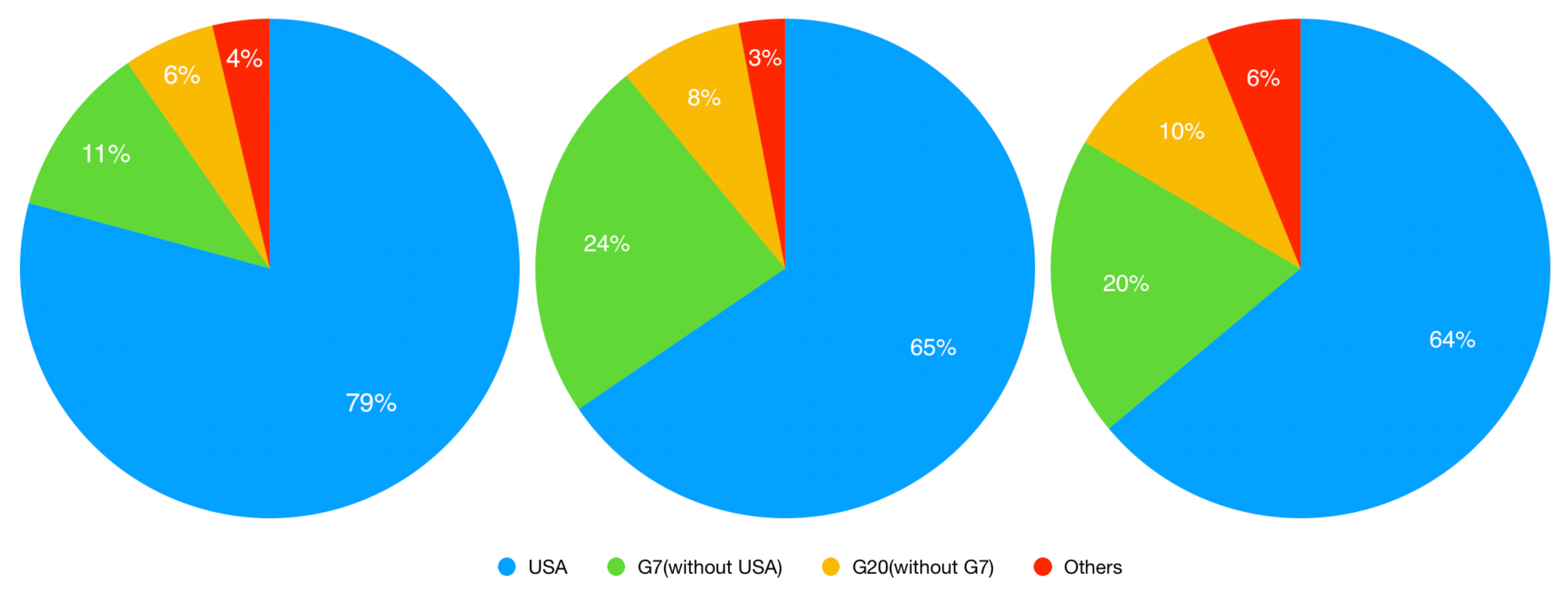
| Period | Country | Minimum | Mean | Median | Maximum |
|---|---|---|---|---|---|
| pre | United States | 0.439 | 0.792 | 0.805 | 0.931 |
| Japan | 0.001 | 0.035 | 0.029 | 0.126 | |
| England | 0.000 | 0.029 | 0.028 | 0.111 | |
| Canada | 0.003 | 0.024 | 0.022 | 0.069 | |
| Russia | 0.000 | 0.014 | 0.010 | 0.105 | |
| in | United States | 0.473 | 0.655 | 0.645 | 0.811 |
| Japan | 0.037 | 0.081 | 0.082 | 0.148 | |
| France | 0.021 | 0.055 | 0.056 | 0.094 | |
| Germany | 0.012 | 0.034 | 0.033 | 0.060 | |
| China | 0.003 | 0.031 | 0.026 | 0.105 | |
| post | United States | 0.468 | 0.652 | 0.639 | 0.929 |
| China | 0.004 | 0.060 | 0.056 | 0.165 | |
| England | 0.008 | 0.049 | 0.050 | 0.105 | |
| Japan | 0.001 | 0.047 | 0.047 | 0.098 | |
| France | 0.008 | 0.039 | 0.039 | 0.066 |
© 2020 by the authors. Licensee MDPI, Basel, Switzerland. This article is an open access article distributed under the terms and conditions of the Creative Commons Attribution (CC BY) license (http://creativecommons.org/licenses/by/4.0/).
Share and Cite
Liu, J.; Song, Q.; Qi, Y.; Rahman, S.; Sriboonchitta, S. Measurement of Systemic Risk in Global Financial Markets and Its Application in Forecasting Trading Decisions. Sustainability 2020, 12, 4000. https://0-doi-org.brum.beds.ac.uk/10.3390/su12104000
Liu J, Song Q, Qi Y, Rahman S, Sriboonchitta S. Measurement of Systemic Risk in Global Financial Markets and Its Application in Forecasting Trading Decisions. Sustainability. 2020; 12(10):4000. https://0-doi-org.brum.beds.ac.uk/10.3390/su12104000
Chicago/Turabian StyleLiu, Jianxu, Quanrui Song, Yang Qi, Sanzidur Rahman, and Songsak Sriboonchitta. 2020. "Measurement of Systemic Risk in Global Financial Markets and Its Application in Forecasting Trading Decisions" Sustainability 12, no. 10: 4000. https://0-doi-org.brum.beds.ac.uk/10.3390/su12104000