Article

Spatial Simulation Modeling of Settlement Distribution Driven by Random Forest: Consideration of Landscape Visibility

1
Center for Applied Geographic Information Science, The University of North Carolina at Charlotte, Charlotte, NC 28223, USA
2
Department of Geography and Earth Sciences, The University of North Carolina at Charlotte, Charlotte, NC 28223, USA
3
Department of Africana Studies, The University of North Carolina at Charlotte, Charlotte, NC 28223, USA
4
Department of Land Resource Management, School of Public Administration, China University of Geosciences, Wuhan 430074, China
*
Author to whom correspondence should be addressed.
Sustainability 2020, 12(11), 4748; https://0-doi-org.brum.beds.ac.uk/10.3390/su12114748
Submission received: 30 March 2020 / Revised: 31 May 2020 / Accepted: 1 June 2020 / Published: 10 June 2020

Abstract

:
Settlement models help to understand the social–ecological functioning of landscape and associated land use and land cover change. One of the issues of settlement modeling is that models are typically used to explore the relationship between settlement locations and associated influential factors (e.g., slope and aspect). However, few studies in settlement modeling adopted landscape visibility analysis. Landscape visibility provides useful information for understanding human decision-making associated with the establishment of settlements. In the past years, machine learning algorithms have demonstrated their capabilities in improving the performance of the settlement modeling and particularly capturing the nonlinear relationship between settlement locations and their drivers. However, simulation models using machine learning algorithms in settlement modeling are still not well studied. Moreover, overfitting issues and optimization of model parameters are major challenges for most machine learning algorithms. Therefore, in this study, we sought to pursue two research objectives. First, we aimed to evaluate the contribution of viewsheds and landscape visibility to the simulation modeling of - settlement locations. The second objective is to examine the performance of the machine learning algorithm-based simulation models for settlement location studies. Our study region is located in the metropolitan area of Oyo Empire, Nigeria, West Africa, ca. AD 1570–1830, and its pre-Imperial antecedents, ca. AD 1360–1570. We developed an event-driven spatial simulation model enabled by random forest algorithm to represent dynamics in settlement systems in our study region. Experimental results demonstrate that viewsheds and landscape visibility may offer more insights into unveiling the underlying mechanism that drives settlement locations. Random forest algorithm, as a machine learning algorithm, provide solid support for establishing the relationship between settlement occurrences and their drivers.

1. Introduction

Land change models are computational approaches that help the investigation of underlying mechanisms of land use and land cover changes to (better) understand a land system of interest. Land change simulation models, as noted by Veldkamp and Fresco [1], “need to integrate different spatial scales and their specific drivers, and should be able to simulate land use/cover changes in response to changes their biophysical and economic/human drivers [2]” (p. 231). These biophysical factors include, but are not limited to, soils, geomorphological, and climate; human factors are exemplified by Gross Domestic Product (GDP) and population [1,3]. A number of land change models have been developed from different disciplines, such as economics, geography, and archaeology [4,5,6].
The topic of land change models in archaeology continues to generate a great deal of interest, especially with modern computers and computational tools that have been made available [7,8]. Land change models provide opportunities for archaeologists to develop a (better) spatial understanding of historical phenomena and their underlying mechanisms. On the other hand, information on how different settlement and land use practices unfolded over time in land change models can be used to guide fieldwork design [9]. In other words, simulation outcome from the land change model is appropriate for designing archaeological survey strategies for locating and studying the settlement patterns of interest. Therefore, land change simulation models provide useful information and decision support that may enable or facilitate new discoveries in archaeological studies. Yet, there are two issues that have been inadequately investigated for land change modeling within the context of archaeology.
The first issue lies in the consideration of landscape visibility in exploring the relationship between the locations of settlement and their driving factors. These driving factors usually reflect characteristics of the environment and human decision-making for the choice of settlement location. Two types of factors drive settlement locations: biophysical drivers (e.g., elevation, slope, and precipitation), and human drivers (e.g., distance to center city, population size). A number of settlement models adopted topographic features as the driving factors, such as elevation, slope, and aspect [10,11]. Distance to water resources and vegetation types also function as driving factors of settlement locations [12,13]. While the importance of these drivers has been well identified in previous studies [10,11,12,13], the consideration of landscape visibility in driving settlement locations is insufficient. Landscape visibility analysis is of essence in guiding human decision-making of settlement location (e.g., for safety and amenity). Landscape visibility analysis (e.g., viewshed analysis) can be seen as an extension of standard biophysical drivers, which is used to investigate global- and local-level characteristics of the landscape within the range of human perception [14]. For example, archaeologists used viewshed analysis to explore intervisibility within settlements [15,16,17]. Thus, landscape visibility analysis provides useful information for understanding underlying mechanisms of settlement locations. However, landscape visibility and associated analysis have been given inadequate attention [18,19], particularly for land change modeling within the context of archaeological studies.
Representation of nonlinearity in complex settlement systems is the second issue. Nonlinearity is a typical property of complex settlement systems [6,20,21]. With the development of computers and techniques, more and more studies adopted cutting-edge approaches to capture nonlinearity in complex settlement systems. Machine learning algorithms are an example of these cutting-edge approaches [22,23,24,25,26,27]. Machine learning algorithms allow us to draw an inference of nonlinear relationships between settlement locations and their drivers. However, some machine learning algorithms (e.g., artificial neural networks) often involve a number of model parameters that need to be calibrated but are difficult to optimize [28]. Meanwhile, overfitting is a common problem in data-driven modeling. How to handle the overfitting issue is still a challenge. Ensemble learning techniques, represented by random forest algorithm [29], have been receiving highlighted interest because they hold great potential in overcoming the overfitting issue. The general idea of an ensemble learning technique is to train multiple models and combine their results into a single output that has better performance on average. For an ensemble learning technique, different models are created for examining the same problem under multiple hypotheses, and a number of combining methods available, such as maximum voting [30,31,32]. Some studies suggested that machine learning algorithms involving ensemble learning techniques can achieve better performance [31,33]. However, a gap between the advancement of machine learning algorithms and how to use these algorithms for real-world applications exists and needs to be filled.
The purpose of this study is thus to address the above two issues by focusing on the following research questions: (1) How should landscape visibility analysis be used in examining the underlying mechanisms of settlement locations, and what is the contribution? and (2) how can land change modeling within the context of archaeological studies benefit from random forest algorithm. We construct a simulation model that integrates random forest algorithm, a representative ensemble machine learning approach, and landscape visibility analysis to study the development of settlement systems. This simulation model is an application of land change modeling in the field of archaeology, and it could be used to design a field survey strategy and draws inferences about human–environment interactions across the landscape. Specifically, we use random forest algorithm to explore the nonlinear relationship between drivers (with the consideration of landscape visibility) and settlement locations during two historical periods—the Stonemarker and Imperial periods in the Western Lower Niger area of Nigeria, West Africa. The remainder of this paper is organized as follows. Section 2 discusses relevant literature and background. Section 3 presents the study area, the dataset related to this study, and design of our simulation model. Section 4 details the experimental design and results. Section 5 presents the discussion. Section 6 summarizes the findings of this study and identifies future work.

2. Literature Review

2.1. Landscape Visibility Analysis

Viewsheds are a component of the landscape that is driven by human–environment interactions. Viewshed analysis is based on “line-of-sight” calculation to determine visible regions on the landscape with respect to a location [14]. The results of viewshed analysis are commonly referred to as viewsheds. Typically, viewsheds are computed by using Geographic Information System (GIS) tools. However, the results of viewshed analysis may vary between different software platforms (contingent on the viewshed algorithms used in these platforms), depending on edge effects (in particular for cumulative viewshed), the quality of terrain data, and the pattern of vegetation. The latter is of particular importance in archaeological studies [34].
Viewshed analysis provides a useful tool in understanding the underlying mechanisms of settlement locations [16,35]. In 1980s, Higuchi and Terry [36] and Antrop [37] showed that intervisibility between settlements and visible areas of territory from the settlements are of importance in studying spatially explicit settlement patterns. Higuchi and Terry defined the “Higuchi Viewshed”, which allows us to investigates the way that we perceive “here” and “there” based on the concept of distance. For “Higuchi Viewshed”, a specific viewshed consists of three visibility zones in terms of the distance: near, middle, and far [36,38,39]. A number of archaeological studies adopted the idea of the “Higuchi Viewshed”, such as Rua et al. [40], Heyns and Van Vuuren [41], and Brughmans et al. [42].
In the past years, researchers have begun to explore ways that viewshed analysis can be integrated into other analyses [16,42,43]. These new viewshed-based methods can enrich and extend current viewshed analysis [17,44]. Moreover, these methods may provide additional information for understanding the locations of settlements [45]. For example, Nutsford et al. developed the “Vertical Visibility Index” (VVI) that calculates vertical degrees of visibility based on standard viewshed analysis results. Their results demonstrated that VVI is of help for improving standard viewshed analysis and provide a better representation of landscape visibility [38]. Meanwhile, some researchers mentioned that quantitative approaches based on viewsheds could be used to evaluate the characteristics of the landscape [46], particularly for settlement study [16,47,48]. Benedikt suggested using spatial characteristics of visibility patterns for describing landscapes [49]. Visibility graph is another example of quantitative approaches as proposed by Turner et al. [50] and O’Sullivan and Turner [51].
Besides, viewshed fragmentation analysis is an extension of standard viewshed analysis. As Gillings mentioned, viewshed fragmentation analysis supports both global and local views [17]. However, in archaeological studies and settlement studies, less attention is paid to viewshed fragmentation analysis. Derivation of landscape metrics and further analysis of these metrics can be used in fragmentation analysis. Landscape metrics are indices that measure the composition and configuration of a landscape within a given area, thus allowing for exploring quantitatively the spatial features of the landscape [52]. However, the applications of landscape metrics in viewshed fragmentation analysis are not sufficient in settlement studies and landscape archaeology. Thus, it is necessary to apply landscape metrics in viewshed fragmentation analysis.

2.2. Random Forest Algorithm

Considering nonlinearity in settlement systems [6,53,54], we use random forest algorithm in our study to capture possible nonlinear relationships between occurrence probabilities and their driving factors. Random forest algorithm, as one of the ensemble machine learning algorithms, has been extensively applied in scientific studies to support, for example, image classification, gene expression classification, and detection and prediction of disease [30,55,56]. Random forest algorithm holds great promise for complex problem-solving through the use of the bagging principle, random sampling of features, and evaluation of feature importance [29]. Additionally, random forest algorithm can overcome overfitting issues because of the ensemble and bootstrapping schemes [29,57,58]. In general, the benefits of random forest algorithm compared with other machine learning algorithms include less proneness to overfitting issues, less pre-defined hyperparameters (to be discussed later), and less computational requirements [59]. However, the application of random forest algorithm has not yet been well utilized in settlement modeling.
Random forest algorithm is a tree-based ensemble learning algorithm that is well tailored to solving classification and regression problems [29]. Random forest algorithm uses bagging predictors as the fundamental mechanism, proposed by Breiman [57]. Bagging is implemented by using a bootstrap sampling strategy, which lies in the resampling a dataset [57]. Two sources of randomness are built in the random forest algorithm: bagging and random input features. Each tree is independently built using bagging, and each node randomly samples a subset of features, instead of all features, to build the tree [29,58].
Generally, the algorithm of random forests consists of a collection of trees that are generated from the datasets (see Figure 1). Each tree contributes a unit vote to predicted class (or prediction) [29,60]. At each tree, the algorithm randomly resamples a training dataset using a bootstrap method (usually this training dataset is called in-bag samples) and selects one dataset or a combination of datasets to build a tree. A series of approaches exist for evaluating the performance of each tree in random forest algorithm, such as Gini and entropy for classification problems [61], and Mean Squared Error (MSE) and Mean Absolute Error (MAE) for regression problems [62]. Out-Of-Bag (OOB) rate is a commonly used index in random forest algorithm to evaluate the testing accuracy of each tree. In random forest algorithm, the OOB rate is calculated using out-of-bag samples (i.e., the samples are dependent with the in-bag samples) as the testing dataset. A higher OOB rate corresponds to a better result.

2.3. Hyperparameter Analysis

In this study, we use a hyperparameter analysis approach to find the suitable hyperparameters of the random forest algorithm for our case study. Hyperparameters are parameters that need to be user-defined or pre-defined before we train a model. For example, the number of trees in a forest is a hyperparameter of random forest algorithm. The choice of hyperparameters can significantly affect the performance of a machine learning algorithm [63,64]. Several studies used machine learning algorithms in different disciplines (e.g., ecology, archaeology, and geography), where trial-and-error and expert opinions are the commonly used methods to identify the appropriate hyperparameters [28]. While the search process of finding the appropriate hyperparameter is a time-consuming task, some search methods can handle the time-consuming issue, such as grid search and random search [63,65]. In grid search, we need to set up a grid of hyperparameter values and every combination of hyperparameters at each grid point is used to train a model. Random search selects random combinations of hyperparameters from the search space.
There are only two hyperparameters in the random forest algorithm: the number of trees in a forest (ntree), and the number of variables randomly sampled as candidates at each split (mtry). The influence and importance of these two hyperparameters have been discussed in the literature [66,67]. In general, the algorithm is more robust with a larger number of trees in the forest. Meanwhile, some studies suggested that mtry has a small effect on the model performance of random forest algorithm [59,66]. However, due to the characteristics of different datasets and models, suggestions from the literature might not be suitable for our model. Moreover, the number of trees in a forest has a direct influence on computing time.
It has been suggested by Breiman [29] that the default parameter setting is to be tried first and then half and twice of the default value for mtry. For the classification problem, the default value of mtry is (Equation (1)):
m t r y = #   v a r i a b l e s   u s e d   i n   t h e   m o d e l
For the regression problem, the default value of mtry is (Equation (2)):
m t r y = # v a r i a b l e s   u s e d   i n   t h e   m o d e l 3
For the number of trees in the forest (ntree), a large number of trees render the model more stable and better estimate the importance of variables, but it is more computationally demaning (in need of more computer memory and running time).

3. Materials and Methods

3.1. Study Area

Our study area is the metropolitan area of the Oyo Empire, crosscutting modern-day Nigeria and the Benin Republic in West Africa in ca. AD 1570–1830 (Figure 2). The Oyo Empire was a trading empire, and the economy was driven mostly by trade, agriculture, and craft and commodity manufacturing, especially cotton textile and iron [68,69]. By contrast, the Stonemarkers (a group of people who lived in the study area between ca. AD 1360 and 1570) pursued a subsistence economy that was likely based on agriculture and pastoralism. The area of our study region is 437.18 km2. In this area, we have identified towns as big as 6.2 km in circumference and 2 km in diameter, which are located within a 20 km radius of Oyo-Ile (the imperial capital)—the capital, 8 × 10 km in size [70].
Part of the case study area is located in Old Oyo National Park across northern Oyo State and southern Kwara State in Nigeria. The Old Oyo National Park lies between latitude 8°15′ and 9° N and longitude 3°45′ and 4°30′ E, covering a total land area of 2512 km2 and sharing boundaries with 11 local government areas. Many settlements surround the park, such as Saki, Iseyin, and Igboho [71].

3.2. Materials

In this study, the Digital Elevation Models (DEM) data that delineate the terrain were taken from the Shuttle Radar Topography Mission (SRTM, https://www2.jpl.nasa.gov/srtm). The spatial resolution of DEM is 1-arc second, or about 30 m (depending on the location on the globe). Figure 2 shows the map of DEM.
Extraction of hydrologic characteristics (e.g., channel network) relies on the principle that an area surrounded by higher elevation values tends to become a sink or channel. However, the topographically derived channel networks do not equal to active streams, since these networks are generated from elevation data instead of real-world observations. Because of lacking stream information in our study area, we assumed the derived channel network is a reasonable representation of active streams. To derive topographic characteristics (e.g., aspect), the elevation value of each foci cell was compared with its neighbors. Thus, the driving factors were derived from DEM, including the location of streams, stream order (stream order is used to measure the size of streams. First-order streams refer to the smallest tributaries with no upstream flow; higher orders correspond to larger tributaries), aspect, slope, and viewsheds (see Table 1). After deriving these factors, all distance-based variables (i.e., proximity variables) were calculated using Euclidean distance. The settlement dataset was digitized based on Google Earth Imagery via visual inspection (we overlaid a 1 km by 1 km lattice on our study area to guide the digitization); the total number of settlements is 362.
Based on the economic features of the pre-imperial and imperial periods, we adopted six driving factors in this study. Figure 3 shows the maps of these factors. Slope represents the steepness at each cell of a surface. The lower the value is, the flatter the terrain. Aspect shows the direction of slope. We expected that slope and aspect play important roles in determining the location of settlements in the study area, because the dominant economic activities in the region were agriculture [69,72]. Regions facing towards south receive more sunlight, thus suitable for agricultural production. Meanwhile, water resource is also expected to be a crucial factor that drives the settlement locations. Viewsheds is used to explore the intervisibility between locations and implications for defense and security as well as territorial control and competitions for natural resources.

3.3. Methods

Simulation models in archaeology have been well studied in the literature [46,73,74]. A suite of simulation models has been developed to support the modeling of settlement occurrence as discrete events. In these simulation models, the occurrence of a settlement is a discrete event controlled by a sequence of events and drivers at a particular time [75]. There are many ways to formulate a discrete-event simulation model (for detailed information see [75]), one of which is to represent how objects and conditions modify the state of the system. Each event occurs at a particular time and triggers a change of the state of the system. The state of the system is also modified by conditions characterized by the driving factors used in the model.
Figure 4 shows the framework of our simulation model, which includes three modules. The first module focuses on landscape visibility analysis. The second module estimates probabilities of the occurrence of settlements using random forest algorithm. Meanwhile, a sub-module, hyperparameter analysis, is added to the estimation of probability-of-occurrence. Hyperparameter analysis helps find the appropriate parameter setting of random forests, which improves the model performance. The spatial allocation module is the third module, and it determines whether a location changes its current state from non-settlement to settlement.
In this study, we involved an extended terrain dataset (30 km of buffer analysis applied here) in order to eliminate the edge effect. To obtain the cumulative viewshed, the number of visible cells for each potential settlement was calculated from all viewpoints on a given terrain dataset, and then they were added together [14]. Further, we used three landscape metrics to measure the spatial characteristics of viewsheds in this study, including perimeter-area fractal dimension (PAFRAC), the number of patches (NP), and aggregation index (AI). PAFRAC was used to examine the shape complexity of the visibility patterns—it approaches 1 for patterns with a simple shape (e.g., a square) and 2 for patterns with a complex shape (e.g., a highly convoluted shape). NP measures the levels of fragmentation. That is, given a specific area, a larger value of NP means the visibility pattern in this area is more fragmented. AI represents levels of aggregation. The larger the value of AI, the more aggregated the pattern is. All the three metrics were calculated at class level. More detailed descriptions of these metrics are provided in McGarigal and Marks [76].
The first step of the framework in this study was to build a transition model to determine whether a non-settlement cell transited to a settlement cell, which is based on random forest algorithm. The transition model is calculated using observed settlements and non-settlement sites (non-settlement sites are randomly selected from the study area). This transition model establishes the relationship between the occurrence of a settlement unit (as a discrete event) and their driving factors. Then, we evaluated the settlement occurrence to generate a spatial map of occurrence probability. In this study, we first generated the initial probability-of-occurrence map as the reference map (t = 0). Then, the candidate pool of potential settlements was generated based on the initial probability-of-occurrence map. The candidate pool was determined by ranking the sites in the reference map based on their probabilities. In other words, the candidates are at the top of the ranking of the occurrence probability; for example, the first N sites from the ranking will be assigned to our candidate pool at time t.
The quantity of new settlements in each simulated time was randomly generated within a range (e.g., 50–300; the range was suggested based on expert opinion). After generating the number of new settlements, we randomly selected a potential site from the candidate pool, and compared the occurrence probability of this site against a random number between 0 and 1 (following a uniform distribution). If the occurrence probability of the site was greater than the random number, the site remained in the pool. Otherwise, it was removed from the candidate pool. All surviving sites were considered as the new settlements at time t + 1. Then, those simulated settlements acted as the existing settlements at time t + 1 to update the map of probability-of-occurrence for time t + 2. The candidate pool was then updated accordingly. This process was repeated until the last simulated time.

3.4. Implementation

All driving factors were derived using the Spatial Analyst toolbox by ArcGIS 10.4 (https://desktop.arcgis.com/en/arcmap/10.4/tools/spatial-analyst-toolbox/an-overview-of-the-spatial-analyst-toolbox.htm). Then, we used Fragstats (version 4.2) [77] to compute landscape metrics for landscape visibility results (https://www.umass.edu/landeco/research/fragstats/fragstats.html). The proposed simulation model was developed using the Python programming language, particularly the scikit-learn library (https://scikit-learn.org/stable/index.html). Although the random forest algorithm is not computationally intensive [59], the random forest algorithm often must be run many times to eliminate the impact of stochasticity. Thus, we involved a parallel computing approach to accelerate the computation. Specifically, we conducted our experiments on the Copperhead computing cluster (Linux-based cluster) in the University Research Computing at the University of North Carolina at Charlotte (https://urc.uncc.edu/). This cluster has 96 computing nodes and 2060 computing cores. The computing nodes that we used in this study have 3.2 GHz of clock rate and 8 GB of memory.

4. Results

4.1. Experimental Design

As discussed, in this study, we designed an experiment to examine the capability of the random forest-driven spatial simulation model. Specifically, we focused on examining the impact of incorporating landscape visibility on settlement location. Our experiment included three treatments. In treatment 1, we only used biophysical factors, including slope, aspect, distance to the nearest streams, and distance to the nearest streams with high order (order > 2). In treatment 2 we added the results of viewshed analysis into the simulation model. Apart from the driving factors used in treatment 2, treatment 3 included the results of viewshed fragmentation analysis (three landscape metrics). Table 2 shows the details of our experiments. We used six simulation periods to investigate the spatial patterns of settlement occurrences: (1) T1, over the next five years; (2) T2, over the next ten years; (3) T3, over the next 15 years; (4) T4, over the next 20 years; (5) T5, over the next 25 years; and (6) T6, over the next 30 years.
To avoid multicollinearity among driving factors, Variance Inflation Factors (VIFs) were calculated, and correlated driving factors were eliminated one by one. That is, we removed the driving factors with high VIF (VIF > 10) one by one [78]. The final models were generated using the following six factors: (1) slope (noted as x1), (2) aspect (noted as x2), (3) distance to the nearest stream (noted as x3), (4) distance to the nearest stream with higher order (order > 2; noted as x4), (5) viewsheds (noted as x5), and (6) PAFRAC (landscape metrics; noted as x6).
For each of the three treatments, we ran the random forest algorithm 100 times. Specifically, we used 100 computing cores to run the random forest algorithm. The total parallel computing time for each treatment (100 runs) was around 140 min based on 100 CPUs. The derivation of viewsheds and landscape metrics is computationally intensive (the parallel computing time is around 150 h with 190 CPUs). For more details, please refer to Zheng et al. [79].

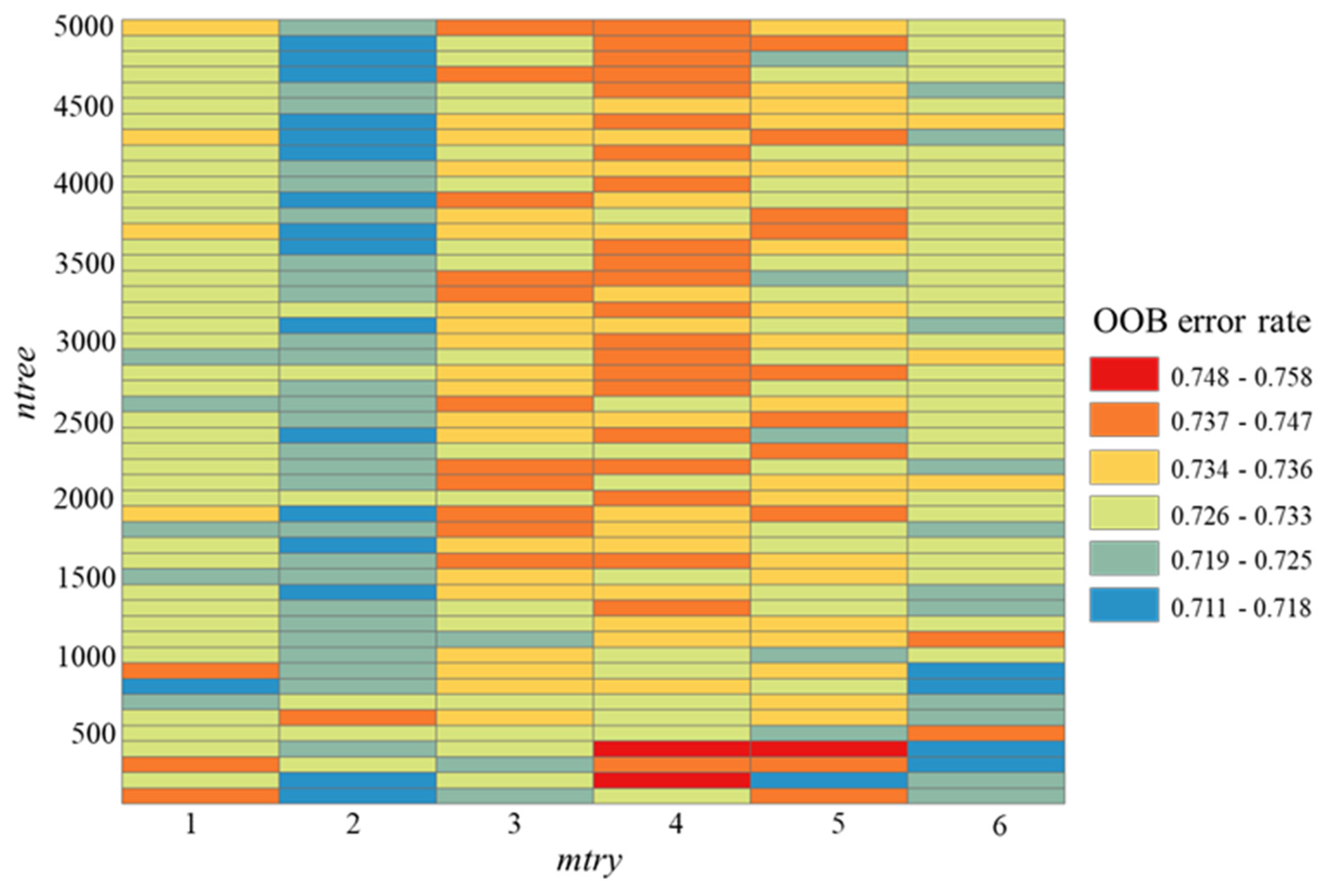
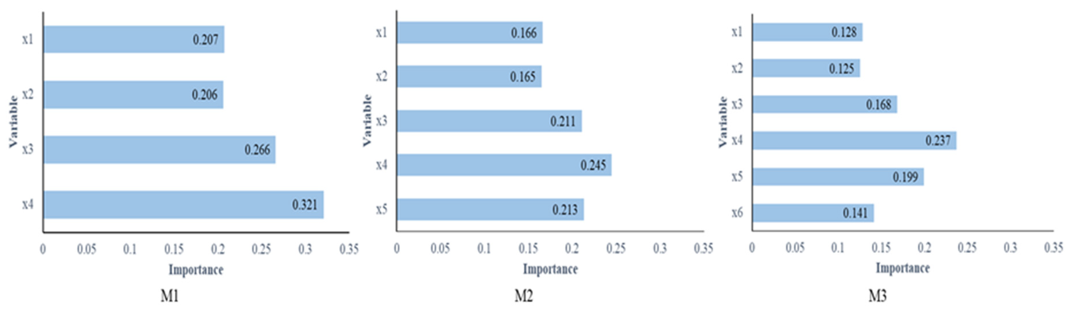
4.2. Results of Hyperparameter Analysis

A grid search method was adopted in this study to find the optimal parameter settings of the random forest algorithm. The selection range of mtry was from 1 to 6 based on Breiman’s suggestion [29]. The ntree ranged from 100 to 5000 with an increment of 500.
Results (Figure 5) from the grid search indicate that the highest OOB error rate (75.8%) was estimated by the combination of an mtry value of 4 with an ntree value of 400. The lowest OOB error rate (71.1%) occurred when mtry was 6 and ntree was 900. Consequently, an mtry value of 4 with an ntree value of 400 were selected as the parameter settings to train the random forest algorithm to simulate the settlement locations in our case study.

4.3. Evaluating the Goodness-of-Fit of the Random Forest Algorithm

In order to evaluate the goodness-of-fit for each treatment, an independent testing dataset (20%; 273 records) was used. In this study, Receiver Operating Characteristics (ROC) curve and the Area Under ROC curve (AUC) values were applied to quantify the performance of our simulation model. The ROC curve is an effective tool for examining the performance for binary classifier systems [80,81]. The ROC curve is a graphical plot that shows the relationship between the true positive rate and false positive rate. The AUC value provides an inference of the robustness of a model. Generally, an AUC for a completely random model is 0.5, and it is 1 for perfect fitting. From Figure 6, we found that the AUC value for treatment M1 was around 0.54, which was slightly better than the completely random model, whereas AUC values for treatment M2 and M3 were 0.667 and 0.691, respectively. All of these AUC values are statistically significant at the 95% confidence interval. Both treatments M2 and M3 had a better fitting performance than treatment M1, and treatment M3 was well explained by the selected driving factors. The AUC statistic summarizes the strength of the overall diagnostic accuracy, and the treatment M3 was the best among the three treatments. Because treatment M3 had the highest goodness of fit among the three treatments, we used the random forest algorithm trained in treatment M3 to drive our final simulation model.
Meanwhile, another quantitative index was used in the random forest algorithm, which is the importance of variables. The importance of a variable is estimated by permuting all variables in the out-of-bag samples. The importance of variables allows us to identify the contributions of each variable in the model [58,59]. In other words, the importance of variables refers to how much a given model relies on this variable to make an accurate prediction. A large value means that the variable has a large contribution to the model. As shown in Figure 7, the distance to the nearest stream with higher order (order > 2) has the most contribution to explaining the likelihood of settlement occurrence in our study region among all treatments, followed by viewsheds and distance to the nearest stream. PAFRAC then made more contributions than slope and aspect. Furthermore, distance to (potential) water resources is the most important component in our settlement model, which is linked to the landscape functioning of our study area (agriculture is one of the economic sources).

4.4. Results of Simulated Settlements

Figure 8 shows the maps of probability-of-occurrence of settlements in our study region. A slight difference can be observed between the reference map and the simulated map. The higher probabilities of settlements concentrate in the lower right corner and the middle of the study area in both cases. Furthermore, locations of higher probabilities were distributed along streams. This finding is a reflection of the results of the importance of variables: the distance to the (potential) water resources has the highest contribution to explaining the occurrence likelihood of settlements in our study region (also see Figure 2). In other words, from the simulation results, access to water resources plays an important role in the settlement development in our study area.
Figure 9 shows the spatial patterns of settlements (including observed and simulated) in our experiment. The lower part of the study region is where the capital of the Oyo Empire is located (preserved region), which explains the existence of few observed contemporary settlements in this area. However, the spatial patterns of the simulated settlements present a different result compared with observed settlements. From a visual inspection, the spatial characteristics of simulated settlements have two patterns: (1) in the north and middle of the study region, simulated settlements exhibit a more dispersed pattern than in lower region; and (2) an aggregated pattern of simulated settlements was observed in the lower region.

5. Discussion

An intensive archaeological survey was undertaken in a small segment of the landscape covered in the simulated study. We wanted to test whether the simulated model is suitable for predicting the settlement pattern of both the pre-Imperial and Imperial periods, or one of them or none. Our survey revealed that the settlement location strategy during the pre-Imperial period, ca. 1360–1570, was different from that of the Imperial period. In the former, settlements were very small and comprised mainly of single house structures and hamlets of 4–7 houses. These pre-imperial settlements (Stonemarker period) are widely dispersed across the landscape. They have been found along the stream channels and at the base and valleys of the granitic hills that are common in the study area (see Figure 9). The archaeological evidence shows that people who lived in these pre-Imperial settlements belonged to the same cultural tradition [72]. They lived in dispersed houses and hamlets, built stone monuments (possibly communal ceremonial centers), and adorned their homes with flatly-laid potsherd pavements. The material culture is minimal, comprising only of small-size pots, querns, and domestic knives. Based on their cultural tradition and natural conditions, we suspect that Stonemarker people may have pursued an agro-pastoral economy, relying more on animal husbandry than farming [69,72]. This would explain the dispersed settlement pattern. Sometimes, we found their settlements near old stream channels or at locations that overlook the valleys. Some of these valleys would have retained water in the past. In other instances, these communities occupied the base of granitic hills farther from any noticeable water sources.
Moving to the Oyo imperial period, the Oyo horsemen and archers recorded swift military victory across a vast territory of the Lower Niger, in the area between present-day southwest Nigeria and eastern Benin Republic, between 1560 and 1570. They consolidated their military conquest by establishing their capital on the very land on which the Stonemarkers had lived for more than 200 years. The settlement pattern of the Imperial Oyo period was very different from the pre-Imperial Stonemarker period. It was characterized by dense urban and village settlements, burnished black and gray wares, and a much more diverse range of artifacts that indicate a very robust market-based economy based on craft specialization, long-distance trade, and agriculture [68,69]. Our archaeological survey in the study region showed that by 1650, what was once a landscape of dispersed small settlements had become one of the largest and densest metropolitan areas in West Africa, comprised of the capital city of 8 × 10 km and a suburb of several densely-populated towns stretching as far as 20 km from the capital. What is striking in this new settlement configuration is that large towns clustered around the base of granitic hills. Surrounding them, in distances of one to seven kilometers, was a satellite of small towns and villages. Some of them specialized in one craft or the other, especially iron-smelting and textile production, while the majority were predominated by farmers. Small settlements such as hamlets and single houses nearly disappeared from the landscape during the Imperial period. There is evidence that levees were built along some of the water channels and drainages were enlarged to divert rainwater from some of the hills to the artificial ponds that were built in the capital city and the adjoining towns. The hills and their slope and aspect, rather than the stream channels, became the overriding factor for settlement location. Our archaeological survey also showed that the summits of these hills were occupied. Defensive walls were built from the lowland up to the summit of some of these granitic hills. The residential structures and artifacts on these hilltop sites show that the inselbergs formed an integral part of the settlement system. Historical sources indicate that contingents of soldiers were sent to the hilltops in rotations to conduct surveillance of the surrounding areas, to watch for intruders and monitor movements of people in and out of the towns and the imperial city.
In the northern part of the study area there is a mismatch between the observed and simulated settlement patterns (Figure 9). One of the reasons is that simulation models are abstractions of the real world, and we cannot avoid assumptions in the simulation models. For instance, in this study, we assumed that the environmental conditions during both the pre-imperial Stonemarker and imperial Oyo periods in ca. 1360–1830 were similar to current conditions. Another reason is that a settlement location is not only determined by the driving factors used in this study, but other factors may also have an influence. For example, regulations can affect settlement locations. For example, the settlement location during the imperial period was significantly influenced by centralized policy decisions. Besides the limitations of the simulation models, there are some limitations of viewshed analysis. For instance, visibility patterns are affected by many aspects, including the quality of terrain datasets, sunlight, the height of the observer, and the radius (i.e., how far can the human eye see).

6. Conclusions

In this study, we proposed a spatial simulation framework that integrates a discrete-event simulation model with random forest algorithm for the study of settlement systems in ancient Oyo, Nigeria. The simulation model in this study introduces the use of viewsheds and spatial metrics of landscape visibility to facilitate the modeling of settlement locations in the study region. Although viewsheds are a valuable property considered in human decision-making of settlement location, consideration of landscape visibility from viewsheds is inadequate in the literature, particularly for land change modeling within the context of archaeological studies. Our experiment demonstrated that viewsheds and landscape metrics of visibility can be of great help in explaining the allocation of settlements driven by human decision-making, which often takes into account, for example, safety or amenity. The use of viewsheds and associated spatial characteristics should be considered in settlement modeling, especially as advanced computing resources become available.
Random forest algorithm, as a machine learning algorithm, provide solid support for establishing the relationship between settlement occurrences and their drivers. This relationship is often nonlinear in complex settlement systems. Hyperparameter analysis helps us determine the appropriate parameters of the random forest algorithm. Results of importance of variables showed that the results of viewshed fragmentation analysis influence the simulated settlement locations in a way comparable to the traditional drivers, such as slope and aspect.
Results in this study provide new insights into studying the settlement locations in the metropolis of the Oyo Empire. Based on our preliminary survey results, the simulated model is appropriate for simulating the pre-Imperial settlement pattern. By contrast, the model is not ideal for predicting the settlement pattern of the Imperial period, during which sociopolitical organization was hierarchical and institutions of social inequality were very well-entrenched. The political elite of the empire played a major role in determining where people lived and who lived where. One of the strategies of maintaining power was to rearrange the demography of the region in ways that served the optimal interest of the political elite. Therefore, settlement location decision was no longer taken at the household level but at the central government level. Not surprisingly, the Imperial-period settlement pattern emphasized security and optimal land use strategies for supporting the population density of the Imperial period. Simulation models give us a tool that can be used to develop a long-term perspective on the ways we view and understand settlement locations. However, due to regulations, social inequality, and types of economic development that are different during the process of social development, the simulation model should consider these changes when developing a long-term perspective.
Future work will focus on collecting more data to evaluate the simulated model, such as land use datasets. Meanwhile, we will incorporate spatially explicit characteristics from the model level. In other words, we will examine how random forest algorithm incorporates spatial characteristics (e.g., neighborhood information within a specific distance). Moreover, settlement systems are complex adaptive systems [7,54]. We will integrate an agent-based model to the modeling framework proposed in this study, because agent-based models allow us to further explore the complexity of human–environment interaction in our study system by taking into account individual-level decision-making.

Author Contributions

M.Z., W.T., and A.O. conceived and designed the experiments. J.Y. and M.Z. collected and analyzed the data. M.Z. performed the experiment. M.Z. wrote the paper with contributions from all other authors. All authors have read and agreed to the published version of the manuscript.

Funding

AO gratefully acknowledges that the archaeological fieldwork component of this study was funded by the American Philosophical Society (Franklin Research Grant) and UNC Charlotte’s Faculty Research Grant.

Acknowledgments

The authors would like to thank five anonymous reviewers. Also, the authors thank Yu Lan for collecting the data used in this study.

Conflicts of Interest

The authors declare no conflict of interest.

References

  1. Veldkamp, A.; Fresco, L. CLUE-CR: An integrated multi-scale model to simulate land use change scenarios in Costa Rica. Ecol. Model. 1996, 91, 231–248. [Google Scholar] [CrossRef]
  2. Turner, B.L.; Moss, R.H.; Skole, D.L. Relating Land Use and Global Land-Cover Change; International Geosphere-Biosphere Programme (IGBP) Secretariat, Royal Swedish Academy of Sciences: Stockholm, Sweden, 1993. [Google Scholar]
  3. Swihart, R.K.; Moore, J.E. Conserving Biodiversity in Agricultural Landscapes: Model-Based Planning Tools; Purdue University Press: West Lafayette, IN, USA, 2004. [Google Scholar]
  4. Hiebeler, D. The Swarm Simulation System and Individual-Based Modeling; Santa Fe Institute: Santa Fe, NM, USA, 1994. [Google Scholar]
  5. Kohler, T.A.; Carr, E. Swarm-based modeling of prehistoric settlement systems in southwestern North America. In Proceedings of the Colloquium II, UISPP, XIIIth Congress, Forli, Italy, September 1996. [Google Scholar]
  6. Tang, W.; Malanson, G.P.; Entwisle, B. Simulated village locations in Thailand: A multi-scale model including a neural network approach. Landsc. Ecol. 2009, 24, 557–575. [Google Scholar] [CrossRef] [PubMed] [Green Version]
  7. Sebastian, L.; Judge, W.J. Predicting the past: Correlation, explanation, and the use of archaeological models. In Quantifying the Present and Predicting the Past: Theory, Method and Application of Archaeological Predictive Modeling; U.S. Department of the Interior, Bureau of Land Management: Washington, DC, USA, 1988; pp. 1–18. [Google Scholar]
  8. Wescott, K.L.; Brandon, R.J. Practical Applications of GIS for Archaeologists: A Predictive Modelling Toolkit; CRC Press: Boca Raton, FL, USA, 2003. [Google Scholar]
  9. Romanowska, I. So you think you can model? A guide to building and evaluating archaeological simulation models of dispersals. Hum. Biol. 2015, 87, 169–193. [Google Scholar] [CrossRef] [PubMed] [Green Version]
  10. Kohler, T.A.; Parker, S.C. Predictive models for archaeological resource location. In Advances in Archaeological Method and Theory; Elsevier: Amsterdam, The Netherlands, 1986; pp. 397–452. [Google Scholar]
  11. Brandt, R.; Groenewoudt, B.J.; Kvamme, K.L. An experiment in archaeological site location: Modeling in the Netherlands using GIS techniques. World Archaeol. 1992, 24, 268–282. [Google Scholar] [CrossRef]
  12. Kohler, T.A.; Kresl, J.; Van West, C.; Carr, E.; Wilshusen, R.H. Be there then: A modeling approach to settlement determinants and spatial efficiency among late ancestral Pueblo populations of the Mesa Verde region, US Southwest. In Dynmics in Human Primate Societies: Agent-Based Modeling of Social and Spatial Processes; Oxford University Press: Oxford, UK, 2000; pp. 145–178. [Google Scholar]
  13. Bi, S.; Ji, H.; Liang, J.; Qiao, W.; Li, X. Spatial distribution of prehistoric settlement sites in Zhengzhou-Luoyang region based on index model. Prog. Geogr. 2013, 32, 1454–1462. [Google Scholar]
  14. Wheatley, D. Cumulative viewshed analysis: A GIS-based method for investigating intervisibility, and its archaeological application. In Archaeology and GIS: A European Perspective; Routledge: London, UK, 1995; pp. 171–186. [Google Scholar]
  15. Gaffney, V.; Van Leusen, P. Extending GIS methods for regional archaeology: The Wroxeter Hinterland Project. In Interfacing the Past: Computer Applications and Quantitative Methods in Archaeology CAA95: Analecta Praehistorica Leidensia 28; Institute of Prehistory: Leiden, The Netherlands, 1996; Volume 2, pp. 297–306. [Google Scholar]
  16. Sevenant, M.; Antrop, M. Settlement models, land use and visibility in rural landscapes: Two case studies in Greece. Landsc. Urban Plan. 2007, 80, 362–374. [Google Scholar] [CrossRef]
  17. Gillings, M. Landscape phenomenology, GIS and the role of affordance. J. Archaeol. Method Theory 2012, 19, 601–611. [Google Scholar] [CrossRef]
  18. Eve, S.J.; Crema, E.R. A house with a view? Multi-model inference, visibility fields, and point process analysis of a Bronze Age settlement on Leskernick Hill (Cornwall, UK). J. Archaeol. Sci. 2014, 43, 267–277. [Google Scholar] [CrossRef] [Green Version]
  19. Brughmans, T.; Brandes, U.J.F.i.D.H. Visibility network patterns and methods for studying visual relational phenomena in archeology. Front. Digit. Humanit. 2017, 4, 17–37. [Google Scholar] [CrossRef] [Green Version]
  20. Van Leusen, P. Line-of-site and cost surface analysis. In Computer Applications and Quantitative Methods in Archaeology; BAR International: Oxford, UK, 1998; pp. 1–8. [Google Scholar]
  21. Ducke, B. Archaeological predictive modelling in intelligent network structures. In The Digital Heritage of Archaeology. Computer Applications and Quantitative Methods in Archaeology; Hellenic Ministry of Culture, Archive of Monuments and Publications: Heraklion, Greece, 2003. [Google Scholar]
  22. Barceló, J.A. Computational intelligence in archaeology. State of the art. In Proceedings of the Making History Interactive. Computer Applications and Quantitative Methods in Archaeology (CAA), Barcelona, Spain, March 1998; pp. 11–21. [Google Scholar]
  23. Venditti, C.P.; Mele, P. Digital Transformation and Archaeology: Innovating Using the Cloud and Artificial Intelligence. In Developing Effective Communication Skills in Archaeology; IGI Global: Hershey, PA, USA, 2020; pp. 224–244. [Google Scholar]
  24. Oonk, S.; Spijker, J. A supervised machine-learning approach towards geochemical predictive modelling in archaeology. J. Archaeol. Sci. 2015, 59, 80–88. [Google Scholar] [CrossRef]
  25. Verhagen, P.; Whitley, T.G. Integrating archaeological theory and predictive modeling: A live report from the scene. J. Archaeol. Method Theory 2012, 19, 49–100. [Google Scholar] [CrossRef] [Green Version]
  26. Czibula, G.; Ionescu, V.-S.; Miholca, D.-L.; Mircea, I.-G. Machine learning-based approaches for predicting stature from archaeological skeletal remains using long bone lengths. J. Archaeol. Sci. 2016, 69, 85–99. [Google Scholar] [CrossRef]
  27. Ren, C.; An, N.; Wang, J.; Li, L.; Hu, B.; Shang, D. Optimal parameters selection for BP neural network based on particle swarm optimization: A case study of wind speed forecasting. Knowl.-Based Syst. 2014, 56, 226–239. [Google Scholar] [CrossRef]
  28. Zheng, M.; Tang, W.; Zhao, X. Hyperparameter optimization of neural network-driven spatial models accelerated using cyber-enabled high-performance computing. Int. J. Geogr. Inf. Sci. 2019, 33, 314–345. [Google Scholar] [CrossRef]
  29. Breiman, L. Random forests. Mach. Learn. 2001, 45, 5–32. [Google Scholar] [CrossRef] [Green Version]
  30. Rodriguez-Galiano, V.F.; Ghimire, B.; Rogan, J.; Chica-Olmo, M.; Rigol-Sanchez, J.P. An assessment of the effectiveness of a random forest classifier for land-cover classification. ISPRS J. Photogramm. Remote Sens. 2012, 67, 93–104. [Google Scholar] [CrossRef]
  31. Ghimire, B.; Rogan, J.; Miller, J. Contextual land-cover classification: Incorporating spatial dependence in land-cover classification models using random forests and the Getis statistic. Remote Sens. Lett. 2010, 1, 45–54. [Google Scholar] [CrossRef] [Green Version]
  32. Gong, Z.; Tang, W.; Thill, J.-C. Parallelization of ensemble neural networks for spatial land-use modeling. In Proceedings of the 5th ACM SIGSPATIAL International Workshop on Location-Based Social Networks, Redondo Beach, CA, USA, November 2012; pp. 48–54. [Google Scholar]
  33. Steele, B.M. Combining multiple classifiers: An application using spatial and remotely sensed information for land cover type mapping. Remote Sens. Environ. 2000, 74, 545–556. [Google Scholar] [CrossRef]
  34. Llobera, M. Modeling visibility through vegetation. Int. J. Geogr. Inf. Sci. 2007, 21, 799–810. [Google Scholar] [CrossRef]
  35. Fry, G.L.; Skar, B.; Jerpåsen, G.; Bakkestuen, V.; Erikstad, L.J.L.; Planning, U. Locating archaeological sites in the landscape: A hierarchical approach based on landscape indicators. Landsc. Urban Plan. 2004, 67, 97–107. [Google Scholar] [CrossRef]
  36. Higuchi, T. The Visual and Spatial Structure of Landscapes; Mit Press: Cambridge, MA, USA, 1986. [Google Scholar]
  37. Antrop, M. Invisible connectivity in rural landscapes. In Proceedings of the 2nd International Seminar of IALE, Connectivity in Landscape Ecology, Munster, Germany, September 1988; pp. 57–62. [Google Scholar]
  38. Nutsford, D.; Reitsma, F.; Pearson, A.L.; Kingham, S.J.A.G. Personalising the viewshed: Visibility analysis from the human perspective. Appl. Geogr. 2015, 62, 1–7. [Google Scholar] [CrossRef]
  39. Wheatley, D.; Gillings, M. Vision, perception and GIS: Developing enriched approaches to the study of archaeological visibility. In Beyond the Map: Archaeology and Spatial Technologies; IPO Press: Amsterdam, The Netherlands, 2000; Volume 321, pp. 1–27. [Google Scholar]
  40. Rua, H.; Gonçalves, A.B.; Figueiredo, R. Assessment of the Lines of Torres Vedras defensive system with visibility analysis. J. Archaeol. Sci. 2013, 40, 2113–2123. [Google Scholar] [CrossRef]
  41. Heyns, A.; Van Vuuren, J. Terrain visibility-dependent facility location through fast dynamic step-distance viewshed estimation within a raster environment. In Proceedings of the 2013 Annual Conference of the Operations Research Society of South Africa, Stellenbosch, South Africa, 15–18 September 2013; pp. 112–121. [Google Scholar]
  42. Brughmans, T.; van Garderen, M.; Gillings, M. Introducing visual neighbourhood configurations for total viewsheds. J. Archaeol. Sci. 2018, 96, 14–25. [Google Scholar] [CrossRef]
  43. Llobera, M. Extending GIS-based visual analysis: The concept of visualscapes. Int. J. Geogr. Inf. Sci. 2003, 17, 25–48. [Google Scholar] [CrossRef]
  44. Gillings, M. Mapping liminality: Critical frameworks for the GIS-based modelling of visibility. J. Archaeol. Sci. 2017, 84, 121–128. [Google Scholar] [CrossRef] [Green Version]
  45. Lake, M.; Ortega, D. Compute-Intensive GIS Visibility Analysis of the Settings of Prehistoric Stone Circles. Comput. Approach. Archaeol. Spaces 2013, 60, 213. [Google Scholar]
  46. Lake, M.W. Explaining the past with ABM: On modelling philosophy. In Agent-Based Modeling and Simulation in Archaeology; Springer: Berlin/Heidelberg, Germany, 2015; pp. 3–35. [Google Scholar]
  47. Jones, E.E. Using viewshed analysis to explore settlement choice: A case study of the Onondaga Iroquois. Am. Antiq. 2006, 71, 523–538. [Google Scholar] [CrossRef]
  48. Gonçalves, C.; Cascalheira, J.; Bicho, N. Shellmiddens as landmarks: Visibility studies on the Mesolithic of the Muge valley (Central Portugal). J. Anthropol. Archaeol. 2014, 36, 130–139. [Google Scholar] [CrossRef]
  49. Benedikt, M.L. To take hold of space: Isovists and isovist fields. Environ. Plan. B Plan. Des. 1979, 6, 47–65. [Google Scholar] [CrossRef]
  50. Turner, A.; Doxa, M.; O’sullivan, D.; Penn, A. From isovists to visibility graphs: A methodology for the analysis of architectural space. Environ. Plan. B Plan. Des. 2001, 28, 103–121. [Google Scholar] [CrossRef] [Green Version]
  51. O’Sullivan, D.; Turner, A. Visibility graphs and landscape visibility analysis. Int. J. Geogr. Inf. Sci. 2001, 15, 221–237. [Google Scholar] [CrossRef]
  52. McGarigal, K. Landscape pattern metrics. In Wiley StatsRef: Statistics Reference Online; Wiley: Hoboken, NJ, USA, 2014. [Google Scholar]
  53. Page, M.; Parisel, C.; Pumain, D.; Sanders, L. Knowledge-based simulation of settlement systems. Comput. Environ. Urban Syst. 2001, 25, 167–193. [Google Scholar] [CrossRef]
  54. Malanson, G.P.; Zeng, Y.; Walsh, S.J. Complexity at advancing ecotones and frontiers. Environ. Plan. A 2006, 38, 619–632. [Google Scholar] [CrossRef]
  55. Qi, Y. Random forest for bioinformatics. In Ensemble Machine Learning; Springer: Berlin/Heidelberg, Germany, 2012; pp. 307–323. [Google Scholar]
  56. Lebedev, A.; Westman, E.; Van Westen, G.; Kramberger, M.; Lundervold, A.; Aarsland, D.; Soininen, H.; Kłoszewska, I.; Mecocci, P.; Tsolaki, M. Random Forest ensembles for detection and prediction of Alzheimer’s disease with a good between-cohort robustness. NeuroImage Clin. 2014, 6, 115–125. [Google Scholar] [CrossRef] [PubMed] [Green Version]
  57. Breiman, L. Bagging predictors. Mach. Learn. 1996, 24, 123–140. [Google Scholar] [CrossRef] [Green Version]
  58. Liaw, A.; Wiener, M. Classification and regression by randomForest. R News 2002, 2, 18–22. [Google Scholar]
  59. Gislason, P.O.; Benediktsson, J.A.; Sveinsson, J.R. Random forests for land cover classification. Pattern Recognit. Lett. 2006, 27, 294–300. [Google Scholar] [CrossRef]
  60. Yue, D.; Peng, C.; Du, D.; Zhang, T.; Zheng, M.; Han, Q. Intelligent Computing, Networked Control, and Their Engineering Applications, In Proceedings of the International Conference on Life System Modeling and Simulation, LSMS 2017 and International Conference on Intelligent Computing for Sustainable Energy and Environment, ICSEE 2017, Nanjing, China, 22–24 September 2017; Springer: Berlin/Heidelberg, Germany, 2017; Volume 762. [Google Scholar]
  61. Pal, M. Random forest classifier for remote sensing classification. Int. J. Remote Sens. 2005, 26, 217–222. [Google Scholar] [CrossRef]
  62. Svetnik, V.; Liaw, A.; Tong, C.; Culberson, J.C.; Sheridan, R.P.; Feuston, B.P. Random forest: A classification and regression tool for compound classification and QSAR modeling. J. Chem. Inf. Comput. Sci. 2003, 43, 1947–1958. [Google Scholar] [CrossRef] [PubMed]
  63. Bergstra, J.; Yamins, D.; Cox, D.D. Making a science of model search: Hyperparameter optimization in hundreds of dimensions for vision architectures. In Proceedings of the ICML’13: the 30th International Conference on International Conference on Machine Learning, Atalanta, GA, USA, June 2013; Volume 28, pp. I-115–I-123. [Google Scholar]
  64. Li, L.; Jamieson, K.; DeSalvo, G.; Rostamizadeh, A.; Talwalkar, A. Hyperband: A novel bandit-based approach to hyperparameter optimization. arXiv 2016, arXiv:1603.06560. [Google Scholar]
  65. Bergstra, J.; Bengio, Y. Random search for hyper-parameter optimization. J. Mach. Learn. Res. 2012, 13, 281–305. [Google Scholar]
  66. Cutler, D.R.; Edwards, T.C., Jr.; Beard, K.H.; Cutler, A.; Hess, K.T.; Gibson, J.; Lawler, J.J. Random forests for classification in ecology. Ecology 2007, 88, 2783–2792. [Google Scholar] [CrossRef] [PubMed]
  67. Strobl, C.; Boulesteix, A.-L.; Kneib, T.; Augustin, T.; Zeileis, A. Conditional variable importance for random forests. BMC Bioinform. 2008, 9, 307. [Google Scholar] [CrossRef] [PubMed] [Green Version]
  68. Agbaje-Williams, B. A Contribution to the Archaeology of Old Oyo; University of Ibadan: Ibadan, Nigeria, 1983. [Google Scholar]
  69. Ogundiran, A. Material life and domestic economy in a frontier of the Oyo Empire during the Mid-Atlantic Age. Int. J. Afr. Hist. Stud. 2009, 42, 351. [Google Scholar]
  70. Agbaje-Williams, B. Field Report: Oyo Ruins of NW Yorubaland, Nigeria. J. Field Archaeol. 1990, 17, 367–378. [Google Scholar] [CrossRef]
  71. Adetoro, A.O. People’s Perceptions of the Old Oyo National Park, Nigeria: Germane Issues in Park Management. Environ. Res. J. 2008, 2, 182–186. [Google Scholar]
  72. Ogundiran, A. The Oyo Empire Archaeological Research Project, 2019 (Third Season): Interim Report of the Fieldwork in Bara, Nigeria, January 11–February 15, 2019. Natl. Comm. Mus. Monum. 2019. Submitted. [Google Scholar]
  73. Doran, J. Systems theory, computer simulations and archaeology. World Archaeol. 1970, 1, 289–298. [Google Scholar] [CrossRef]
  74. Kohler, T.A. Putting social sciences together again: An introduction to the volume. In Dynamics in Human and Primate Societies: Agent-Based Modelling of Social and Spatial Processes; Oxford University Press: Oxford, UK, 2000; pp. 1–44. [Google Scholar]
  75. Banks, J. Handbook of Simulation: Principles, Methodology, Advances, Applications, and Practice; John Wiley & Sons: Hoboken, NJ, USA, 1998. [Google Scholar]
  76. McGarigal, K.; Marks, B.J. Fragstats: Spatial Pattern Analysis Program for Quantifying Landscape Structure. Reference Manual; Forest Science Department, Oregon State University: Corvallis, OR, USA, 1994; Volume 62. [Google Scholar]
  77. McGarigal, K.; Cushman, S.A.; Ene, E. FRAGSTATS: Spatial Pattern Analysis Program for Categorical and Continuous Maps; Computer Software Program; Version 4; University of Massachusetts: Amherst, MA, USA, 2012. [Google Scholar]
  78. O’brien, R.M. A caution regarding rules of thumb for variance inflation factors. Qual. Quant. 2007, 41, 673–690. [Google Scholar] [CrossRef]
  79. Zheng, M.T.; Wen, w.; Ogundiran, A.; Chen, T.; Yang, J. Parallel landscape visibility analysis: A case study in archaeology. High Perform. Comput. Geospatial Appl. 2020, in press. [Google Scholar]
  80. Hajian-Tilaki, K. Receiver operating characteristic (ROC) curve analysis for medical diagnostic test evaluation. Casp. J. Intern. Med. 2013, 4, 627. [Google Scholar]
  81. Pumain, D. Settlement systems in the evolution. Geogr. Ann. Ser. B Hum. Geogr. 2000, 82, 73–87. [Google Scholar] [CrossRef] [Green Version]
Figure 1. Structure of a random forest algrotihm (M: the number of datasets used in a study; N: total number of records of the input; Z: number of records of the subset that is less than or equal to N; V, X, and G are the numbers of datasets used in the tree, and each of them is less than or equal to M; in-bag sample is the training sample in the tree (two thirds of the records of the subset), whereas out-bag sample is the testing sample (one third of the records of the subset)).
Sustainability 12 04748 g001
Figure 2. Study area in this study.
Sustainability 12 04748 g002
Figure 3. Selected driving factors used in this study.
Sustainability 12 04748 g003
Figure 4. Framework of the simulation model in this study (t is the current simulated year; T is the last simulated year).
Sustainability 12 04748 g004
Figure 5. Results of hyperparameter analysis of random forest algorithm (OOB: Out-Of-Bag; mtry: the number of variables randomly sampled as candidates at each split; ntree: number of trees in the forest).
Sustainability 12 04748 g005
Figure 6. Receiver Operating Characteristics (ROC) curves and Area Under ROC (AUC) values for the simulation model based on the testing dataset (M1–3 are treatment IDs, see Table 2 for detail).
Sustainability 12 04748 g006
Figure 7. The importance of variables in the random forest model (x1: slope; x2: aspect; x3: distance to the nearest stream; x4: distance to the nearest stream with higher order (order > 2); x5: viewsheds; x6: perimeter-area fractal dimension (PAFRAC)).
Sustainability 12 04748 g007
Figure 8. Probability-of-occurrence maps of settlements (T0, current time; T6, over next 30 years).
Sustainability 12 04748 g008
Figure 9. Spatial patterns of observed and simulated settlements (left: the locations of observed settlements; right: the locations of simulated settlements using treatment M3; T1–T6 are simulation times, see Section 5 for details).
Sustainability 12 04748 g009
Table 1. Datasets used in this study. SRTM: Shuttle Radar Topography Mission; DEM: Digital Elevation Models.
DatasetsUnitDescriptionSource
DEMMeterelevationSRTM
SlopeslopeDerived from DEM
AspectDecimal degreeaspectDerived from DEM
StreamMeterdistance to the nearest streamDerived from DEM
Stream (order > 2)Meterdistance to the nearest stream with higher order (order > 2)Derived from DEM
Viewshednumber of visible settlementsDerived from DEM
Settlements (including different types, such as towns, villages, and hamlets)1 = settlement,
0 = non-settlement
whether the place is a settlementDigitized from Google Earth
Table 2. Design of the experiment in this study.
Treatment IDDriving Factors
M1Slope, aspect, distance to the nearest stream, distance to the nearest stream with higher order (order > 2)
M2Slope, aspect, distance to the nearest stream, distance to the nearest stream with higher order (order > 2), viewsheds
M3Slope, aspect, distance to the nearest stream, distance to the nearest stream with higher order (order > 2), viewsheds, landscape metrics

