A Quantitative Analysis of the Optimal Energy Policy from the Perspective of China’s Supply-Side Reform


1
School of Economics, Peking University, Beijing 100871, China
2
School of Environmental Science and Engineering, Shanghai Jiaotong University, Shanghai 200240, China
*
Author to whom correspondence should be addressed.
Sustainability 2020, 12(12), 4800; https://0-doi-org.brum.beds.ac.uk/10.3390/su12124800
Submission received: 6 May 2020
/
Revised: 29 May 2020
/
Accepted: 3 June 2020
/
Published: 12 June 2020
Abstract
:How does the capacity removal policy affect China’s economy? To quantify the policy outcomes and costs, a four-sector model with vertical market structures is built. The calibrated model shows that, to achieve the policy goal, 10% of equipment operation in the high energy-consuming sectors must be shut down. This policy leads to an improved energy structure in which total energy consumption drops by 4.75% at the cost of a contraction in economic growth, where the total output declines by 12.31%. The numerical experiments find that the optimal policy is to limit the production scale in both the iron/steel industry and the fossil energy industry, closing 9% and 7% of the production, respectively, since doing so minimizes output loss and improves the energy structure. This paper quantifies the impact of the current capacity removal policy and provides policy alternatives to reach the same policy target with a lower output loss.

1. Introduction
China has been growing rapidly in recent decades, but, due to government intervention and overinvestment, some industries have experienced overcapacity. The severe imbalance of supply and demand in traditional sectors will create social problems, such as market depression and environmental pollution [1]. To control and resolve overcapacity issues, the PRC government implemented a command-and-control policy for supply-side reform in 2015 that aims to stabilize the market and lead the shift to a clean energy structure by reducing production in critical sectors [2]. It is vital to understand how this policy is taking effect and how high the policy cost is.
To quantify the impact of the capacity removal policy, this paper builds a four-sector model with a vertical market structure. The model has the following key features. First, it distinguishes high energy-consuming sectors and low energy-consuming sectors according to the energy intensity proposed by Gutowski [3]. Second, both fossil energy producers and green energy producers are introduced in the model. The energy sectors respond to the capacity removal reform, although the policy applies to the intermediate goods sectors. Third, the model captures the path dependency and spillover effect of the innovation process in the energy sectors. The reform improves the energy structure and relocates scientists and workers between the two types of energy firms.
The model is calibrated to match the salient features of China before the reform. This paper matches the capital share of the energy sector and scientific efficiency. Moreover, the model can match the untargeted moments in the data, such as the ratio of the capital share in fossil energy production to that in green energy production. Then, the model is calibrated to evaluate the effects of the capacity removal policy.
The quantitative results show that, to achieve the capacity removal goal of 8% in the high energy-consuming sectors, 10% of equipment operation must be shut down. Because of the vertical market structure, total energy consumption drops by 4.75%, with high energy-consuming industries using 6.55% less energy. The total output decreases by 12.31%.
This paper compares a few different policy alternatives that achieve the same goal. The numerical results show that the policy of closing 9% of the intermediate goods sector and 7% of the energy sector is the optimal policy since it leads to the largest green energy consumption share and smallest output loss.
The main contributions of this paper comprise three aspects. First, a structural model is constructed to quantify the impact of the capacity removal policy. Second, the calibrated model well matches the stylized facts in China. Finally, this research finds the best governing strategy and provides quantitative advice for capacity removal policy in China. It proposes three policy schemes to attain the same capacity removal target and proves that each policy will achieve the goal at the cost of short-term pain.
2. Literature
This paper is related to works discussing excess production capacity in China. Researchers have studied these issues considering three aspects: (1) analysis of the reasons for excess production capacity in relevant Chinese industries [1,4,5]; (2) calculation of the existing capacity utilization and prediction of the scale of future excess production capacity [6,7,8,9]; and (3) provision of policy suggestions that address excess production capacity [10,11]. This paper complements the existing studies by quantifying the policy impact.
This work builds on the literature that focuses on directed technical change and climate policy. Most earlier works are mainly theoretical (e.g., [12,13,14,15]). Only a few papers closely related to quantitative analyzation have been published. To calculate the amount of abatement from a given sized carbon tax, a climate-economy model is developed by Goulder [16]. A DICE model is modified by Popp [17] to find that appropriate policies can help achieve a given emissions target at a small expense of social welfare. Another macro model also proposed that, given a fixed target of emissions abatement, the tax requirement under a technical incentive policy is much lower(Gerlagh [18]).
This paper extends the model proposed in the existing literature. The endogenous technology setting is inherited from Acemoglu [19], and the model structure shares some features of Fried [20], who set the machine manufacturer as the upstream innovation sector. However, the presented model incorporates R&D into the production function of the energy sector directly. This change is essential to study how the capacity removal policy affects technological advancement in the energy sector. The model details are shown in Appendix A.
This paper uses numerical methods to analyze different environmental policies; this approach is connected to papers such as those by Heutel [21], Fischer [22], and Angelopoulos [23]. In particular, Dissou [24] extended the previous works by studying the different shock impacts occurring in the multi-sector model.
The previous literature did not explain the model from the perspective of energy structure optimization. After implementation of the capacity removal policy, the green energy output rises sharply, and the fossil energy output falls severely. At the same time, the relative price advantage of green energy steadily increases. These changes in output and price show that the policy optimizes the energy structure, which is a novel perspective from which to interpret the effects of China’s capacity removal policy.
3. Model
To understand the impact of the capacity removal policy, a structural model is required to evaluate how this policy affects sectors along the production chain. Additionally, the model should provide a framework to find the optimal policy for achieving the goals of capacity removal.
This work extends the model of Fried [20], assuming innovation to be in the manner of Acemoglu [19]. There are four sectors, within which the markets for energy producers and energy suppliers are both monopolistic, which mimics China’s energy market structure. Furthermore, the vertical sector structure enables analysis of how the capacity removal policy affects the production chain. (A descriptive diagram is provided in the Appendix A, Appendix B and Appendix C).
3.1. Final Goods
The final goods (Y) are produced with two elements: high energy-consumption materials (M), with steel being the main material, and low energy-consumption materials (N). The production function is assumed to be in the form of CES. Final goods are consumed by households or used for energy production. In the following equation, represents the distribution of high energy-consumption materials and is the output elasticity of substitution.
3.2. Intermediate Goods
Intermediate goods consist of high energy-consumption materials and low energy-consumption materials , both of which have a Cobb–Douglas production function. () represents the labor share of high (low) energy-consumption materials.
The inputs to intermediate production are labor (L) and energy (E). Labor is rented at wage rates , and the prices of the raw materials are denoted as and . (Both the final goods and the intermediate goods markets are perfectly competitive. Parameter represents the share of energy output and represents the share of labor output). The maximization problem for high energy-consumption materials is
and similar for low energy-consumption materials. In equilibrium, .
3.3. Energy Producer
The energy producer is a complete monopoly intermediate provider. Energy (E) is a nested CES composite of fossil energy (F) and green energy (G). (Since is a function of and , the method of implicit differentiation is utilized to calculate the derivative of the energy price relative to its production). represents the distribution of fossil energy and is the energy elasticity of substitution.
The provider purchases fossil and green energy from the energy manufacturers and generates energy for the downstream sectors. Given energy price , the maximization problem of the energy producer is as follows.
3.4. Energy Producer
Fossil and green energy are produced with only capital inputs:
where variable is the invested final goods and denotes the technology embedded in energy production. This work follows the convention of Fried [20] to model the dynamics of the technology evolution,
For each sector, the productivity level in period t is determined by two channels. The first channel is path dependency, indicating that the productivity level in the current period is partially determined by the productivity level in the previous period. The second channel is known as the knowledge spillover effect brought about by employed scientists, , and the average productivity level in the energy sector.
Parameter measures the efficiency of scientists creating new inventions and implies that there are diminishing returns on the investment of employing scientists. Parameters and are introduced to govern sector diversity. (Considering the diversity within the industry is particularly important since the return on innovation in both industries is decreasing. Without diversification, the marginal output of scientists in the fossil energy sector is much lower than that in the green energy sector because the fossil energy sector is much larger).
As the technology spills over from one sector to another, this paper uses to denote how sector j’s innovation affects all industries. Sector productivity in the current period will boost productivity in the next period. Parameter captures the intensity of the spillover effect.
Aggregate productivity is calculated as the weighted average of productivity in each department. Following Fried [20], parameters and represent the number of processes that have the potential for innovation by scientists in fossil and green industries, respectively.
Given the energy selling price and the wage of scientists , the energy producer maximizes its profit.
3.5. Market Clearing
- Intermediate goods market.
- Energy market. In equilibrium, the energy demand for the two types of intermediate products should be equal to the energy output.
- Labor market. The supply of workers L is normalized to 1, which equals the number of workers employed by high and low energy-consuming firms.The supply of scientists S is exogenously calibrated to match the ratio of scientists to workers. (The number of scientists refers to actual staff with college degrees or higher working in the energy sector).
4. Numerical Results
Numerical experiments were implemented to answer the following questions: (1) What are the effects of the capacity removal policy on efficiency, especially the cross-sector impact? (2) Is there an alternative policy tool that can achieve the same policy goal? To address these questions, the model is calibrated to match the key variables in the data and numerical exercises were performed for quantitative analysis.
4.1. Calibration and Model Validation
This paper calibrates the model to match the Chinese data. It splits the timeline into two periods, before and after 2015, which is the year in which the Chinese government implemented the structural reform policy. The first period represents the balanced growth path (BGP), which lasted 10 years, and the second period is the shock period, which lasted from 2015 to 2017. The basic parameters are calibrated with the Newton iterative method in the BGP period as a benchmark, and its outputs are used as the initial inputs of the shock period to analyze the shock effects.
The data used here come from two main sources. The basic macro index data, such as the value added of secondary industry Y, numbers of employees in the steel industry and in the whole secondary industry ( and L, respectively) and industrial energy consumption (E), come from the China National Bureau of Statistics. Most of the data in the energy industry are from China’s Industrial Statistics Yearbook of the same period (from 2006 to 2017). These data include energy consumption in the iron and steel industry () and the energy generation, R&D investment ( and ) and capital input ( and ) of fossil and green energy, respectively. Then, the total fossil (or green) energy generation is multiplied by the proportion of industrial power consumption to calculate the fossil (or green) energy generation for industrial purposes as the corresponding variable F (or G) in the model. The proportion of R&D investment in fossil (or green) energy companies in the whole industry is also multiplied by the number of scientists in the energy industry to calculate the number of scientists in the fossil (or green) industry as the variable (or ) in the model.
The parameter values of , and come directly from the literature. The parameter values of , , and S are computed from the data. The parameters, including , , and , are jointly calibrated by the method of moments to capture the relationships between energy production and price.
The calibration strategy (a detailed discussion of the calibration can be found in the Appendix A, Appendix B and Appendix C) well matches the ratio of energy consumption of industry M, the ratio of energy supply of industry F, the ratio of scientists in industry G and the scientist structure of the energy production sector (see Table 1 and Table 2 for details).
4.2. Quantitative Results
In 2016, the China State Council issued Suggestions on Excess Production Capacity and Overcoming Development Dilemmas in the Iron and Steel Industry, setting the policy objective of reducing steel production capacity by 100 million tons within three years. According to the data from the National Bureau of Statistics, by the end of 2015, steel production had reached 1.2 billion tons in China. The aim of the production reduction policy is to lower the output of high energy-consuming industries by approximately 8%.
The calibrated model was used to conduct numerical experiments. In the benchmark experiment, the implementation of the production removal policy was simulated in the following three experiments with the same target: reducing the production of the high energy-consuming industry by 8%. (This experiment could be interpreted as the outcome of the capacity removal policy).
4.3. Experiment
Experiment 1
As shown in Equation (20), the objective of production decline is attained by the capacity reduction in downstream material industries with high energy consumption.
The policy impact intensity parameter is calibrated to mimic the scale of the production shutdown for the target of an 8% decrease in production. (The parameter value ranges between 0 and 1. If the original level of the production line is 1, then is the level of the production line after production declines. The decrease in the production line can lead to a declining demand for energy and an increased demand for labor as an alternative). The calibration results of imply that, by closing down 10% of equipment operation (the shutdown of equipment leads to a drop in energy consumption) in material industries, the policy target of reducing the output of material industries by 8% can be obtained.
Compared with the BGP period, the price of high energy-consumption material increases by 10.79%, indicating that the policy of production reduction attains the stated objectives of raising prices in the steel market and improving the situation of industries.
Second, the gross output Y declines by 12.31%, showing the negative impact of the production reduction policy on aggregate output. Total power generation E drops by 4.75%. Energy consumption in high energy-consuming industries declines by 6.55%, while energy consumption in low energy-consuming industries decreases by 27.51%.
Finally, upstream sectors achieve productivity improvement. Gross productivity A increases by 9.76%. Scientists relocate from fossil energy industries to green energy industries. Hence, the productivity of green energy industries is improved more significantly than that of fossil energy industries.
In summary, Experiment 1 attains the government goals of “raise steel price and improve industrial situation”, as mentioned in the government supply reform. In addition, it also facilitates the shift to a clean energy structure and technological innovation in the energy sectors. However, the targets are achieved at a high cost in terms of total output decline.
Experiment 2
To find better policy alternatives, a second experiment was performed, implementing a production removal policy in the upstream sector. In Experiment 2, the objective of production decline (M decreases by 8%) is attained by capacity reduction in the fossil energy industry of the upstream sector.
To achieve the policy goal of reducing the output of material industries by 8%, 12% capacity in the fossil energy industry must be removed, which requires a greater shutdown than that in Experiment 1.
The following results are similar to those in Experiment 1. (1) The prices of high energy-consumption materials increase by 9.54%, which is slightly less than the increase in Experiment 1. This increase is mainly caused by additional links of transmission. (2) The energy structure (G/(F+G)) is increased by 20.32%, which is less significant than that in Experiment 1. (3) Gross output Y declines by 13.83%, leading to higher policy costs. (4) The gross productivity A of the energy sectors increases by 9.97%, which is slightly greater than that in Experiment 1. The main reason is that the policies have direct influences on the energy sectors.
The effect of imposing a production removal policy in the fossil energy industry is slightly inferior, and the policy cost is slightly higher.
Experiment 3
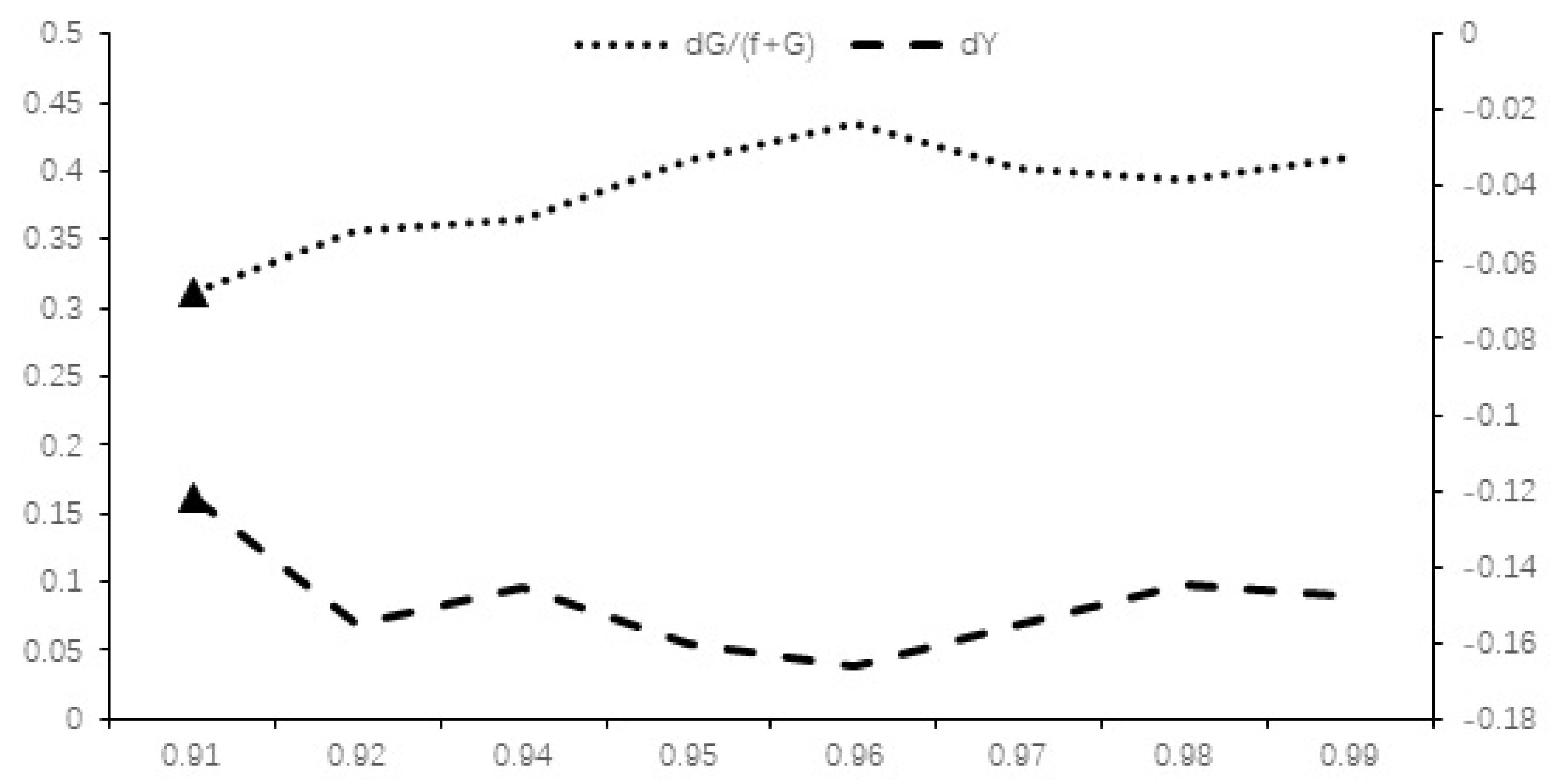
To find a better policy, shocks are introduced in both the fossil energy industry and the material industry with high energy consumption. Experiments with different combinations of and were performed to achieve the same goal of reducing the output of the material industries by 8%. As shown in Figure 1, when one sector is exposed to a more severe shock, the other sector must be allowed to increase production.
Figure 2 shows that the policy of has the most significant effect. The energy structure (G/(F+G)) is increased by 31.26%. In addition, the green energy relative price / increases by 31.26%. This policy also has a minimum aggregate output cost: gross output Y decreases by only 12.18%, which is the least among the three experiments.
The paper finds that the three policy schemes attain the basic target of supply reform. In addition, they all facilitate a shift to a clean energy structure and technological innovation in the energy sectors. However, the targets are attained at a policy cost of a decrease in gross output. By comparing the three experiments, this paper finds that the composite policy in Experiment 3 simultaneously maximizes the share of green energy and minimizes the decrease in gross output. Subsequent facts (according to the 2019 Work Report of the Chinese government, deepened supply-side reform and promotion of the implementation of market-oriented capacity reduction policies in the steel and coal industries are supported) also prove that, during the critical period of supply reform, the government of China should adopt a composite policy of simultaneous reduced production in the upstream and downstream sectors to optimize the reform process, amplify the results of the reform and ensure quality completion as scheduled. More results are provided in the Appendix A, Appendix B and Appendix C.
5. Conclusions
This paper analyzes the impact of the production capacity removal policy that was implemented in China in 2015. This paper builds a structural model with four sectors, calibrates the model to mimic China’s economy and shows that the policy removes excess production capacity at the cost of GDP loss but simultaneously optimizes the energy structure. The numerical experiments suggest that removing some production capacity in both the high energy-consuming sector and the fossil energy sector can achieve the same policy goal at a smaller cost.
This paper abstracts from some interesting and important aspects that could affect the evaluation of the supply-side reform. For example, the endogenous interest rate could add general equilibrium effects to the analysis. Industry policy will affect people’s occupational choices as well as innovation and productivity. All these features can be incorporated into future research.
Author Contributions
Conceptualization, B.L., H.W. and J.X.; methodology, B.L. and J.L.; formal analysis, H.W. and J.X.; writing–original draft preparation, H.W. and J.X.; writing–review and editing, B.L. and J.L. All authors have read and agreed to the published version of the manuscript.
Funding
This research was funded by School of Economics, Peking University and National Natural Science Foundation of China (NSFC), Grant No. 71810107001 and 71690241.
Acknowledgments
Bo Li thanks School of Economics, Peking University for Research Support. Jingyu Liu is Supported by National Natural Science Foundation of China (NSFC), Grant No. 71810107001 and 71690241.
Conflicts of Interest
The authors declare no conflict of interest.
Appendix A. A Descriptive Diagram
Figure A1.
Descriptive diagram of the production chain.

Appendix B. Computation
The main equations are derived in this text. The final goods producer chooses M and N to maximize its profit.
The first-order condition implies that tax-inclusive prices and are functions of the intermediate goods.
The intermediate goods producers in the perfect competition market use labor L and electricity E as input factors to maximize profit-taking prices as given below.
The first-order condition shows the relationship between factor price and product price.
The energy producer is monopolistic. It uses fossil and green energy to generate electricity E and attempts to pursue maximum profits.
To derive the first-order condition, the derivation method for the implicit function must be used because is also a function of , which has a CES form of and . This work denotes as the derivative of with respect to and and as the derivatives of with respect to and . The first-order condition is shown as (A11) and (A12)
The energy producer hires scientists to develop new technologies, which can promote the efficiency of fossil and green energy generation.
The producers of fossil and green energy are also monopolistic. As a result, the derivative of with respect to and the derivative of with respect to must be calculated. The symbols , , and are used for simplicity.
The first-order condition for the energy sector is shown as (A19)–(A22).
Appendix C. Results

Table A1.
Variable value changes from the BGP to the shock period.
| BGP | Experiment 1 | Experiment 2 | Experiment 3 | |
|---|---|---|---|---|
| Gross output:Y | 0.348 | 0.305 | 0.300 | 0.306 |
| (−12.31%) | (−13.83%) | (−12.18%) | ||
| Fossil energy:F | 0.391 | 0.417 | 0.420 | 0.403 |
| (6.72%) | (7.56%) | (3.28%) | ||
| Green energy:G | 0.424 | 0.534 | 0.513 | 0.557 |
| (66.36%) | (53.67%) | (76.09%) | ||
| Energy structure:G/(F+G) | 0.288 | 0.478 | 0.442 | 0.506 |
| (26.02%) | (20.90%) | (31.26%) | ||
| Energy:E | 0.495 | 0.472 | 0.431 | 0.462 |
| (−4.75%) | (−13.00%) | (−6.78%) | ||
| Scientists in industry F: | 0.006 | 0.004 | 0.004 | 0.005 |
| (−28.23%) | (−28.71%) | (−18.89%) | ||
| Scientists in industry G: | 0.004 | 0.005 | 0.006 | 0.005 |
| (28.73%) | (39.41%) | (18.07%) | ||
| Technology of industry F: | 2.212 | 2.378 | 2.377 | 2.394 |
| (7.48%) | (7.44%) | (8.21%) | ||
| Technology of industry G: | 1.818 | 2.054 | 2.065 | 2.038 |
| (13.03%) | (13.63%) | (12.11%) | ||
| Technology of industry G:A | 2.038 | 2.237 | 2.241 | 2.239 |
| (9.76%) | (9.97%) | (9.85%) | ||
| Price of industry M: | 0.522 | 0.578 | 0.572 | 0.577 |
| (10.79%) | (9.54%) | (10.50%) | ||
| Price of industry F: | 0.360 | 0.394 | 0.488 | 0.401 |
| (9.45%) | (35.50%) | (11.33%) | ||
| Price of industry G: | 0.423 | 0.371 | 0.472 | 0.356 |
| (−12.12%) | (11.73%) | (−15.80%) | ||
| Relative energy price:/ | 1.173 | 0.0.941 | 0.967 | 0.887 |
| (−19.71%) | (−17.55%) | (−24.37%) |
References
- Zhang, Y.; Zhang, M.; Liu, Y.; Nie, R. Enterprise investment, local government intervention and coal overcapacity: The case of China. Energy Policy 2017, 101, 162–169. [Google Scholar] [CrossRef]
- Boulter, J. China’s Supply-side Structural Reform. Reserve Bank-Aust. Bull. 2018, 12, 1–19. [Google Scholar]
- Gutowski, T.G.; Sahni, S.; Allwood, J.M.; Ashby, M.F.; Worrell, E. The energy required to produce materials: Constraints on energy-intensity improvements, parameters of demand. Philos. Trans. R. Soc. Lond. Ser. A 2013, 371, 001–003. [Google Scholar] [CrossRef] [PubMed]
- Lin, J.Y.; Wu, H.-M.; Xing, Y. “Wave Phenomena” and Formation of Excess Capacity. Econ. Res. J. 2010, 10, 4–19. [Google Scholar]
- Wang, Y.; Luo, G.; Guo, Y. Why is there overcapacity in China’s PV industry in its early growth stage? Renew. Energy 2014, 72, 188–194. [Google Scholar] [CrossRef]
- Feng, Y.; Wang, S.; Sha, Y.; Ding, Q.; Yuan, J.; Guo, X. Coal power overcapacity in China: Province-Level estimates and policy implications. Resour. Conserv. Recycl. 2018, 137, 89–100. [Google Scholar] [CrossRef]
- Wang, D.; Wang, Y.; Song, X.; Liu, Y. Coal overcapacity in China: Multiscale analysis and prediction. Energy Econ. 2018, 70, 244–257. [Google Scholar] [CrossRef]
- Yuan, J.; Li, P.; Wang, Y.; Liu, Q.; Shen, X.; Zhang, K.; Dong, L. Coal power overcapacity and investment bubble in China during 2015–2020. Energy Policy 2016, 97, 136–144. [Google Scholar] [CrossRef]
- Yang, Q.; Hou, X.; Han, J.; Zhang, L. The drivers of coal overcapacity in China: An empirical study based on the quantitative decomposition. Resour. Conserv. Recycl. 2019, 141, 123–132. [Google Scholar] [CrossRef]
- Wang, D.; Wan, K.; Song, X.; Liu, Y. Provincial allocation of coal de-capacity targets in China in terms of cost, efficiency, and fairness. Energy Econ. 2019, 141, 109–128. [Google Scholar] [CrossRef]
- Li, W.; Lua, C.; Ding, Y.; Zhang, Y. The impacts of policy mix for resolving overcapacity in heavy chemical industry and operating national carbon emission trading market in China. Appl. Energy 2019, 204, 509–524. [Google Scholar] [CrossRef]
- Acemoglu, D. Directed technical change. Rev. Econ. Stud. 2002, 4, 781–809. [Google Scholar] [CrossRef] [Green Version]
- Smulders, S.; De Nooij, M. The impact of energy conservation on technology and economic growth. Resour. Energy Econ. 2003, 1, 59–79. [Google Scholar] [CrossRef] [Green Version]
- Acemoglu, D.; Akcigit, U.; Hanley, D.; Kerr, W. Transition to clean technology. J. Political Econ. 2016, 1, 53–104. [Google Scholar] [CrossRef] [Green Version]
- Hart, R. Directed technological change: It’s all about knowledge. Swed. Univ. Agric. Sci. Dep. Econ. Work. Pap. Ser. 2012, 2, 1–18. [Google Scholar]
- Goulder, L.H.; Stephen, H.S. Induced technological change and the attractiveness of CO2 abatement policies. Resour. Energy Econ. 1999, 21, 211–253. [Google Scholar] [CrossRef]
- Popp, D. ENTICE: Endogenous technological change in the DICE model of global warming. J. Environ. Econ. Manag. 2004, 48, 742–768. [Google Scholar] [CrossRef] [Green Version]
- Gerlagh, R. A climate-change policy induced shift from innovation in carbon-energy production to carbon-energy savings. Energy Econ. 2008, 30, 425–448. [Google Scholar] [CrossRef]
- Acemoglu, D.; Aghion, P.; Bursztyn, L.; Hémous, D. The Environment and Directed Technical Change. Am. Econ. Rev. 2012, 1, 131–166. [Google Scholar] [CrossRef] [PubMed] [Green Version]
- Fried, S. Climate policy and innovation: A quantitative macroeconomic analysis. Am. Econ. J. Macroecon. 2018, 1, 90–118. [Google Scholar] [CrossRef] [Green Version]
- Heutel, G. How should environmental policy respond to business cycles? Optimal policy under persistent productivity shocks. Rev. Econ. Dyn. 2012, 2, 244–264. [Google Scholar] [CrossRef] [Green Version]
- Fischer, C.; Springborn, M.R. Emissions targets and the real business cycle: Intensity targets versus caps or taxes. J. Environ. Econ. Manag. 2011, 3, 352–366. [Google Scholar] [CrossRef]
- Angelopoulos, K.; Economides, G.; Philippopoulos, A. What is the Best Environmental Policy? Taxes, Permits and Rules under Economic and Environmental Uncertainty. Athens Univ. Econ. Bus. DEOS Work. Pap. 2010, 3, 1–37. [Google Scholar]
- Dissou, Y.; Karnizova, L. Emissions cap or emissions tax? A multi-sector business cycle analysis. J. Environ. Econ. Manag. 2016, 79, 169–188. [Google Scholar] [CrossRef] [Green Version]
Figure 1.
Values of and .

Figure 2.
Combination of shocks and policy effects.

Table 1.
Value of the method of moments in the data and model.
| Method of Moments | Data | Model |
|---|---|---|
| Ratio of energy consumption of industry M: /E | 0.73 | 0.73 |
| Ratio of energy supply of industry F: F/E | 0.80 | 0.79 |
| Ratio of scientists in industry G: /S | 0.41 | 0.43 |
| Scientist structure of the energy production sector: / | 1.44 | 1.33 |
Table 2.
Calibration results for parameter values.
| Parameter | Value | Source |
|---|---|---|
| Final goods production | ||
| Output elasticity of substitution: | 0.95 | — |
| Distribution of high energy-consumption materials: | 0.6 | Data |
| Intermediates production | ||
| Labor share of high energy-consumption materials: | 0.19 | Data |
| Labor share of low energy-consumption materials: | 0.49 | Data |
| Number of workers: L | 1 | Normalization |
| Production shock of sector M in policy 1: | 0.90 | Method of moments |
| Production shock of sector F in policy 2: | 0.88 | Method of moments |
| Production shock of sector M in policy 3: | 0.91 | Method of moments |
| Production shock of sector F in policy 3: | 0.93 | Method of moments |
| Energy production | ||
| Capital share of fossil energy: | 0.915 | Method of moments |
| Capital share of green energy: | 0.599 | Method of moments |
| Energy supply | ||
| Energy elasticity of substitution: | 1.5 | Literature |
| Distribution of fossil energy: | 0.5 | — |
| Research | ||
| Cross-sector spillovers: | 0.5 | Literature |
| Diminishing returns: | 0.79 | Literature |
| Scientist efficiency: | 6.017 | Method of moments |
| Sector size of fossil producers: | 1 | Normalization |
| Sector size of green producers: | 0.773 | Data |
| Number of scientists: S | 0.01 | Data |
© 2020 by the authors. Licensee MDPI, Basel, Switzerland. This article is an open access article distributed under the terms and conditions of the Creative Commons Attribution (CC BY) license (http://creativecommons.org/licenses/by/4.0/).
Share and Cite
MDPI and ACS Style
Xi, J.; Wu, H.; Li, B.; Liu, J. A Quantitative Analysis of the Optimal Energy Policy from the Perspective of China’s Supply-Side Reform. Sustainability 2020, 12, 4800. https://0-doi-org.brum.beds.ac.uk/10.3390/su12124800
AMA Style
Xi J, Wu H, Li B, Liu J. A Quantitative Analysis of the Optimal Energy Policy from the Perspective of China’s Supply-Side Reform. Sustainability. 2020; 12(12):4800. https://0-doi-org.brum.beds.ac.uk/10.3390/su12124800
Chicago/Turabian StyleXi, Jianming, Hanran Wu, Bo Li, and Jingyu Liu. 2020. "A Quantitative Analysis of the Optimal Energy Policy from the Perspective of China’s Supply-Side Reform" Sustainability 12, no. 12: 4800. https://0-doi-org.brum.beds.ac.uk/10.3390/su12124800
Note that from the first issue of 2016, this journal uses article numbers instead of page numbers. See further details here.