Article

Has China’s Emission Trading System Achieved the Development of a Low-Carbon Economy in High-Emission Industrial Subsectors?

1
School of Economics and Management, Taiyuan University of Technology, Taiyuan 030024, China
2
Department of International Trade, Inha University, Inharo100, Nam-gu, Incheon 402-751, Korea
*
Authors to whom correspondence should be addressed.
Sustainability 2020, 12(13), 5370; https://0-doi-org.brum.beds.ac.uk/10.3390/su12135370
Submission received: 27 May 2020 / Revised: 25 June 2020 / Accepted: 30 June 2020 / Published: 2 July 2020
(This article belongs to the Special Issue Energy Efficiency and Urban Climate Adaption)

Abstract

:
An emission trading system (ETS) is a powerful emission reduction tool for achieving low-carbon economic development in the world. Focusing on the industrial subsectors, this paper comprehensively analyzes the environmental and economic effects of the pilot ETS in China from the perspectives of economic development, technological optimization, and innovation-driven development by using the propensity score matching–difference in differences (PSM-DID) model based on 2005–2017 provincial panel data. This paper compensates for the limitations of existing studies on the effects of ETS on different subsectors; furthermore, the triple difference model (DDD) model is used to discuss the impacts of differences in environmental responsibility and economic potential among subsectors on policy effects. The empirical results show that: (1) The pilot ETS produces a 14.5% carbon reduction effect on the covered subsectors while reducing GDP by 4.8% without achieving a low-carbon economy. Thus, production decline is the main reason for carbon emission reductions. (2) Economic development factors have significant positive impacts on carbon emissions, while technological optimization and innovation-driven development are key factors for achieving reductions in carbon emissions. (3) The pilot ETS produces a 60.1% carbon emission inhibition effect and 23.2% GDP inhibition effect on the subsectors with greater environmental responsibility. Therefore, the Chinese government should fully simulate the impact of technological innovation and utilize resource endowment differences in the environmental and economic aspects of different sectors to achieve low-carbon economic development.

1. Introduction

Global climate change poses a major environmental threat to the sustainable development of society, while the main cause is excessive greenhouse gas emissions. To cope with global climate change, major countries in the world have adopted different measures and policy combinations to achieve energy conservation and emissions reduction targets such as renewable energy subsidies, non-fossil energy replacement, building and equipment efficiency standards, energy intensity targets, differential electricity prices, environmental and resource taxes, and national emission trading systems (denoted as ETS) [1]. An ETS is a key market-based policy tool for addressing climate change and includes legislative mechanisms, industry coverage, quota allocation methods, monitoring and verification systems, historical data accounting, and specific set-off rules [2]. An ETS is also a powerful way for all countries to reduce their greenhouse gas emissions and thus mitigate climate change [3].
As the largest carbon emitter in the world, China is clearly a main part of the international carbon emission trading market [4]. It was in recognition of this that the National Development and Reform Commission of China submitted plans to implement the pilot ETS in 2011, which was launched in seven regions since 2013, i.e., Beijing, Tianjin, Shanghai, Chongqing, Guangdong, Hubei, and Shenzhen. Together, these pilot projects involve 1.2 billion tons of carbon dioxide emissions from different sectors, which exceeds all other emission trading mechanisms in the world except for the European Union’s ETS [5]. These pilot projects have gradually expanded nationwide since 2017. They initially incorporated approximately 3.5 billion tons of carbon dioxide emissions from more than 1700 companies, mainly from the power sector. The transaction volume will surpass EU’s ETS to become the largest ETS in the world [6]. The Chinese government has made clear the need for a green, open, and innovation-driven low-carbon economy. The industrial sector contributes more than 40% of the GDP, consumes more than 70% of China’s total energy consumption, and occupies a dominant position in China’s ETS. It is essential to point out that China’s first seven pilot regions actually cover eight subsectors, and, except for the air transport sector, the other seven subsectors all belong to industry (see Appendix A for the details). Could these industrial subsectors achieve low-carbon economic development through the pilot ETS? To answer this research question, this study attempts to assess the environmental and economic effects of ETS on the actual coverage of industrial subsectors in the pilot areas and analyzes the key influencing factors. China’s ETS will gradually upgrade from a regional ETS to a national ETS; the differences in resource endowments among different subsectors in provincial regions will inevitably increase the uncertainty for the successful implementation of a national ETS, at which point the different emitters will need to assume “common but differentiated responsibilities” to achieve the national emission reduction target [7]. Considering the differences between historical emission liabilities and economic development capacities, this paper investigates whether there are significant differences in environmental responsibility and economic potential among provincial subsectors and discusses their ultimate impact on policy effects, which is another objective of this research.
Next, this paper examines relevant precedent studies which include ETS in major countries around the world and focuses on related research and the modeling methods of China’s ETS, as well as on case studies in the included industrial subsectors. Verbruggen et al. provided a preliminary analysis of the four main components of EU’s ETS: emission reduction measures, regulatory measures, carbon price levels, and emission reduction costs; they found that to achieve the coexistence of the industrial low economy pressure target and the low-carbon environment target, the applicability of the existing ETS needed to be discussed in depth on the basis of its specific design structure [8]. Nguyen et al. used Japan as an example and assessed the economic viability and environmental efficiency of ETS. Their results show that modest carbon prices and inelastic constraints could reduce carbon emissions by 42%, while the best combination of elastic methods could reduce emissions by 34% [9]. Nong et al. assessed the impact of the Australian ETS on carbon emissions and economy and found that carbon prices will gradually increase from 4.1 Australian dollars/ton in 2015 to 41.3 Australian dollars/ton in 2030 and that the 28% carbon emission reduction target by 2030 compared to 2005 is achievable. Meanwhile, GDP is expected to decrease by 1.6% in 2030 [10]. Oke et al. and Diaz et al. conducted similar studies on ETS of sustainable development in South Africa and low-carbon development in New Zealand, respectively [11,12].
From the statistics of international energy agencies, which show global carbon emissions of up to 31.6 billion tons in 2012, the developed countries have achieved less than 20% of the global reduction target, while developing countries are responsible for the rest. As the largest developing country, China accounts for nearly 50% of the world’s potential for emission reductions [13]. Therefore, many scholars have used relevant models to study the policy effects of China’s ETS, mainly discussing the environmental and economic effects. Wang et al. used inter-provincial panel data to analyze the policy effects of the pilot ETS by using the propensity score matching-difference in differences model (denoted as PSM-DID). Their results indicated that the ETS could achieve both environmental and economic benefits and the low-carbon economy transformation target [14]. Yu et al. used the data envelopment analysis model (denoted as DEA) to analyze the potential benefits of the ETS and found that it generated a 21.0% average potential environmental benefit and a 92.0% average potential economic benefit for industry [15]. Liu et al. adopted the computable general equilibrium model (denoted as CGE) and analyzed the environmental and economic effects for Hubei province as the exemplary pilot area. Their results indicated that in 2014, the ETS reduced the carbon emissions of Hubei by 1%, while the economy decreased by 0.06% [16]. Some scholars have used hybrid models in their research. For instance, Zhu et al. combined the PSM-DID model with the DEA model and discussed the impacts of the ETS on green development efficiency in China. Their conclusions show that the ETS has a significant positive impact of 4.25% on green development efficiency [17]. Zhang et al. combined the DID model with the stochastic frontier approach (denoted as SFA) and analyzed the effects of the pilot ETS on carbon intensity and carbon emissions. It was found that the pilot ETS decreased industrial carbon intensity and carbon emissions by 0.78% and 10.1%, respectively [18]. As can be seen from the above literature, scholars mainly used the DID, DEA, and CGE models from a bottom-up perspective, to analyze the policy effects of ETS regions and whole sectors in China. Almost all of the studies found that the ETS had a significant inhibitory impact on carbon emissions, but the conclusions related to economic effect were different [19,20,21,22,23,24]. In 1991, Porter proposed that reasonable environmental regulations could send positive signals to enterprises, that resource allocations were inefficient and that the technology needed to be improved, which would autonomously stimulate the “innovation compensation” effect. Therefore, Porter’s hypothesis could not only offset the “compliance cost” of enterprises but also achieve both environmental and economic benefits by improving productivity and international competitiveness [25]. This raises the question of whether the industrial subsectors covered by China’s ETS can achieve a win-win situation for the environment and the economy by promoting technological optimization and innovation-driven development. To answer this question, the limited literature, which discussed the policy effects of ETS in specific coverage sectors, mainly began at the enterprise and subsector levels. Focusing on the panel data of listed enterprises in seven energy-intensive industries in China from 2010 to 2017, Zhang and Liu used the DID model to select the listing age, firm size, capital structure, liquidity, and R&D investment to analyze the economic effect of ETS on enterprises. Their conclusions indicated that the regulatory policy had a positive economic impact on electric power enterprises and a negative economic impact on non-ferrous metal enterprises, and thus showed clear industrial heterogeneity; it had positive economic impacts on paper production and aviation enterprises with a lag of two to four years and showed long-term profitability on the whole [26]. Zhang et al. used the same method and selected the listing age, per capita fixed assets, and enterprise ownership to discuss the effects of ETS on technological innovation by enterprises; they found that the policy had positive impacts on the technological innovation of power and aviation enterprises but had negative impacts on the other six industries and thus indicated clear heterogeneity [27]. There was also research on the total factor productivity of manufacturing enterprises, denoting that the ETS did not achieve the ideal “Porter effect” [28]. The literature from the enterprise perspective mainly concluded that ETS policy effects have significant industrial heterogeneity for the listed enterprises in the covered industries and mainly selected financial indicators to analyze specific reasons such as the scale of the enterprise and the years of listing. Zhang et al. used the DEA model to analyze policy effects on carbon emissions and GDP in industrial subsectors. They concluded that the time-restricted sector trading scenario and the unrestricted sector trading scenario had positive impacts on industrial added value of 55.17% and 73.76%, respectively, from 2006 to 2015, and reduced carbon emissions by 58.30% and 65.25%, respectively [29]. Focusing on the panel data of inter-provincial industrial subsectors from 2005 to 2015, Zhang and Duan used the DID model to select the output, state-owned asset ratios, fixed asset ratios, and profitability as control variables to discuss the effects of ETS on the total output and employment of industrial subsectors. Their conclusion is noteworthy in that the pilot ETS significantly reduced GDP and would lead to significant employment declines in related subsectors, but would not produce a “decoupling” of carbon emissions and GDP in the short term [30]. Zhang et al. used the DID model and selected the same control variables to analyze the effects of ETS. Their conclusion demonstrated that China’s ETS would reduce carbon emissions and show an increasing trend over the years but would fail to effectively reduce the carbon intensity of the covered subsectors. They further found that the main reason for reductions in carbon emissions was to reduce production, so the proportion of free quota should be tightened to facilitate technological innovation and effectively reduce carbon intensity in the future [31]. The literature on the effects of ETS on the covered sectors has also mainly selected relevant financial indicators for analysis and argued that the ETS could promote different levels of carbon emission reductions, but there are some disagreements regarding whether the economic effect could be achieved.
To summarize, the literature on the policy effects of ETS was mainly based on whole sectors in China and relevant pilot areas. As sector studies focused on the industrial sectors with the highest emission levels, research on the specific coverage of ETS in China was sufficiently in-depth; the research methods used mainly included the DID, DEA, and CGE models, and there was little research using multiple models from different perspectives. Previous research has mainly addressed the environmental and economic effects of ETS, and much of this research concluded that an ETS will produce significant emission reductions, but the economic effect remains to be studied. In view of the complexity of data collection, the variables selected by the relevant literature for industrial subsectors were relatively few in number, as the financial indicators were mainly selected at both the enterprise and departmental levels. These studies were less concerned with significant technical and innovation indicators to achieve low-carbon economic development, and thus had certain limitations.
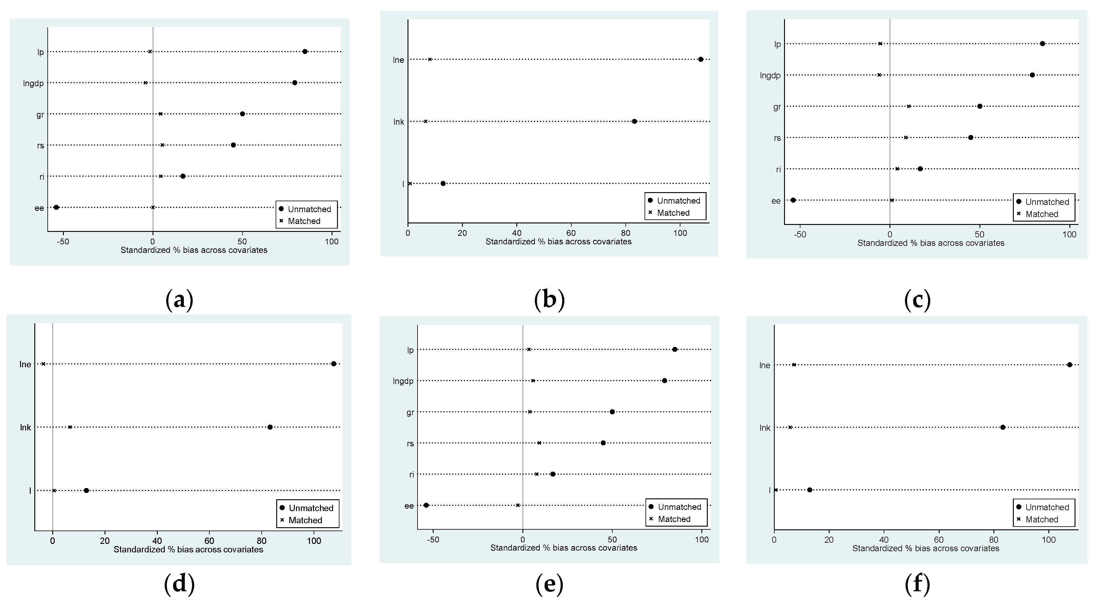
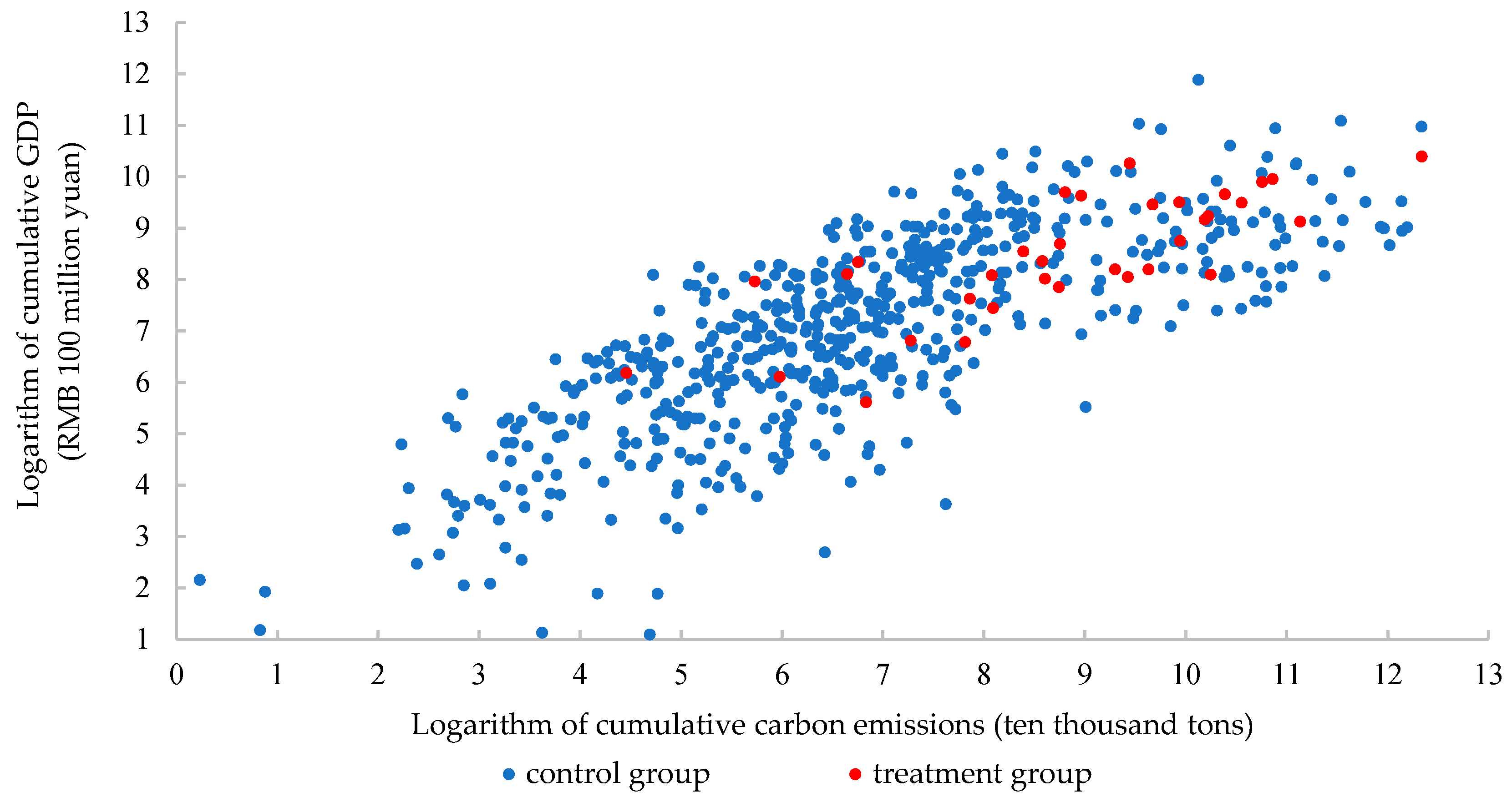
Based on the existing research results, this paper makes three main contributions. First, instead of examining the provincial industrial sector as a whole, because China’s ETS initially covered the industrial high-emission subsectors of the pilot areas, provincial industrial sectors are subdivided into 37 subsectors, according to the industrial classification code of national economic activities (GB/T 4754-2011), and seven industrial subsectors involved in the pilot areas are defined as the treatment group and reflect the actual coverage of the pilot ETS. Second, while most studies used a single model, we used both the PSM-DID model according to different matching methods, to eliminate the selection bias of large sample sets, and the triple difference model (denoted as DDD), introduced on the basis of PSM-DID research to construct a new control group to fix trend differences, thereby obtaining unbiased estimations of the treatment effect [32]. Third, while previous studies on industrial subsectors mainly chose the financial indicators, from the perspectives of economic development, technological optimization, and innovation-driven development, we used the panel data of provincial subsectors from 2005–2017 to select representative variables, in order to analyze the environmental and economic effects of the pilot ETS from multiple perspectives. More importantly, on the basis of the above results, we considered the differences in environmental responsibility and economic potential among subsectors, and then evaluated the influence of developmental heterogeneity on the ultimate policy effects, which are further discussed by considering the imbalance of resource endowments among different subsectors to provide supporting evidence for the national ETS future plan in China.
The remainder of this research is organized as follows. In Section 2, the research design, methods, and data are introduced. In Section 3, empirical results are presented, including PSM matching results, DID benchmark regression results, a robustness test, and the triple difference model (DDD) regression results. Then we discuss and analyze all these empirical results and propose some implications and suggestions. In Section 4 the conclusion of the research is summarized, putting forward the policy proposals.

2. Research Design and Methodology

2.1. Research Design

The seven pilot areas covered by the ETS in China have different geographical locations, carbon emissions, and gross economies, but all pilot areas follow the principle of “invigorating the large ones while relaxing small ones”, and mainly cover sectors with strong development endowments and great emission reduction potential [33,34]. Instead of viewing all sectors as a whole, this study focuses on the industrial high-emission subsectors covered by the pilot ETS policy in China; the pilot ETS is viewed as a “quasi-experiment” and take the included industrial subsectors in the pilot areas as the treatment group, while the industrial subsectors not included in other areas are set as the control group (see Appendix A for the details). From the perspectives of economic development, technological optimization, and innovation-driven development, representative indicators are exploited to compare the changes of carbon emissions and GDP before and after the pilot ETS. Thus, the environmental and economic benefits of ETS in China are analyzed. By illustrating the environmental responsibility-economic potential distribution map of industrial subsectors, the impacts of developmental differences on the ultimate effects of the pilot ETS are further discussed based on the above regression results.

2.2. Methodology

2.2.1. PSM-DID Model

The DID model is widely used to evaluate the effectiveness of sociological public policy implementations. The basic idea is to divide samples into the treatment group, with policy intervention, and the control group, without policy intervention. If there is no significant difference between both of these groups before and after the policy shock, this implies that the change of intervention policies has no significant effect on the treatment group (counterfactual results). If this is not the case, the actual effect of the policy shock can finally by obtained by comparing the trend differences between the treatment group and the control group [35,36]. In order to avoid any bias in the group samples, the PSM model is further utilized to examine the differences of samples before and after matching, for the potential deviations according to different matching methods. Thus, the PSM-DID model constructs a random assignment experiment and ensures effective estimations [37]. Compared with other methods related to policy effectiveness, the synthetic control method (denoted as SCM) requires for the counterfactual weight to be kept within the non-negative interval of 0–1. If the gap of the treatment group is significantly different from that of the control group, a suitable counterfactual set will not be obtained, and thus the SCM requires a long time span of samples before and after policy intervention. It is difficult to construct an ideal control group to reflect the actual implementation effect of the policy in practice [38], because the difference between the regression discontinuity model (denoted as RD) and the DID model lies in the definition of dummy variables. Thus, the RD model needs to find the critical point between the treatment and control groups, and then the effect of policy intervention is inferred based on the change of the samples on both sides of this critical point. The final outcome will only apply to the samples interval around the critical point and the existing limitations of external validity will evolve accordingly [39]. In this research, the seven industrial subsectors covered by the pilot areas are set as the treatment group, while those industrial subsectors not covered in other areas are set as the control group, and dummy variables are introduced in the experimental period. Considering the actual situation of the pilot ETS in Hubei and Chongqing, and in order to entirely reflect the actual policy effects of the pilot ETS, we take 2014 as the baseline year of the pilot. In view of this, we first use different PSM methods to verify whether the pilot ETS is a randomized assignment experiment; then, by gradually adding different control variables, the environmental and economic effects are estimated by regression. The complete DID model is as follows.
C it = α 0 + α 1 subs i * peri t + α 2 Control it + η i + γ t + μ it
Y it = β 0 + β 1 subs i * peri t + β 2 Control it + η i + γ t + μ it
Here, Cit and Yit are the environmental effect dependent variable and the economic effect dependent variable of the pilot ETS of industrial subsector i in year t, respectively. Subsi is the subsector dummy variable; if industrial subsector i belongs to the subsectors included in the pilot ETS, subsi = 1, otherwise subsi = 0; perit is the time dummy variable; if it belongs to the pilot ETS implementation year, i.e., 2014–2017, perit = 1; otherwise perit = 0, i.e., 2005–2013. “Control” reflects the control variables of environmental effect and economic effect, respectively; η is the subsectors’ fixed term; γ is the time fixed term; and μ is the time disturbance term. Therefore, the interaction term “Z = subsi*perit” we are concerned with is represented by the environmental treatment effect and economic treatment effect of the industrial subsectors included in the pilot ETS in the experimental period after excluding the time trend differences.

2.2.2. DDD Model

The hypothesis of the common trend of the DID model requires that any change in the treatment group be the same as that in the control group before the experiment. Otherwise, the DDD model should be introduced to control trend differences and to achieve unbiased estimations of treatment effect by constructing a new control group. Based on the above DID estimation results, to further analyze the influence mechanism of environmental responsibility difference and economic potential difference among industrial subsectors on the final implementation effects of the pilot ETS, the environmental responsibility difference dummy variable and economic potential difference dummy variable are introduced. The triple difference model is constructed as follows.
C it = α 0 + α 1 subs i * peri t * if _ c j + α 2 subs i * peri t + α 3 subs i * if _ c j + α 4 peri t * if _ c j + α 5 control it + η i + γ t + μ it
Y it = β 0 + β 1 subs i * peri t * if _ c j + β 2 subs i * peri t + β 3 subs i * if _ c j + β 4 peri t * if _ c j + β 5 control it + η i + γ t + μ it
C it = α 0 + α 1 subs i * peri t * if _ g j + α 2 subs i * peri t + α 3 subs i * if _ g j + α 4 peri t * if _ g j + α 5 control it + η i + γ t + μ it
Y it = β 0 + β 1 subs i * peri t * if _ g j + β 2 subs i * peri t + β 3 subs i * if _ g j + β 4 peri t * if _ g j + β 5 control it + η i + γ t + μ it
Here, if_c is the dummy variable of environmental responsibility difference and if_g is the dummy variable of economic potential difference. By selecting cumulative carbon emissions and the cumulative GDP of various industrial subsectors to represent environmental responsibility and economic potential, if the cumulative carbon emissions and the cumulative GDP of industrial subsector j from 2005 to 2017 rank at the top 50% of all industrial subsectors in a region, the corresponding dummy variables if_c and if_g are both set to 1, otherwise they are taken as 0. Other variable settings are the same as for the DID model. We are also interested in the triple interaction term “Z = subsi*perit*if_c” or “Z = subsi*perit*if_g”, which is further discussed in the developmental differences among industrial subsectors on the final effects of the pilot ETS. Through the interaction term “Z = subsi*perit”, we can judge whether development heterogeneity of subsectors exists among different regions and the validity of the introduced DDD model.

2.3. Data and Variables

According to the research design in Section 2.1, this research first adopts the industrial classification code of national economic activities (GB/T 4754-2011), dividing provincial industries into specific subsectors and removing most of the subsectors for which the observed values are zero. Moreover, panel data from 37 industrial subsectors from 2005–2017 are selected. When considering data availability, detailed subsector energy consumptions are not given in the statistical yearbooks of Shanghai, Jiangsu, Zhejiang, Sichuan, and Xizang. And detailed subsector R&D data are not provided in the statistical yearbooks of Inner Mongolia, Liaoning, Jilin, Anhui, Jiangxi, Hainan, Guizhou, Qinghai, and Ningxia. Data of Shenzhen comes from Guangdong’s statistical yearbook. Therefore, this study involves the seven industrial subsectors included in the pilot areas taken as the treatment group, i.e., Beijing, Tianjin, Chongqing, Hubei, and Guangdong; and the other excluded industrial subsectors of the above five areas and remaining twelve areas were taken as the control group, i.e., Hebei, Shanxi, Heilongjiang, Fujian, Shandong, Henan, Hunan, Guangxi, Yunnan, Shaanxi, Gansu, and Xinjiang (see Appendix A for the details). Some missing data were supplemented by interpolation methods, and the logarithmic transformation of related variables was used to eliminate heteroscedasticity. Meanwhile, to prevent outliers, we truncated the corresponding quantiles of 5% and 95% of the variables involved in the panel data and ultimately obtained data for 3438 available non-zero annual provincial industrial subsectors.

2.3.1. Indicators of Environmental Effect

As the calculation of carbon emissions contains both fossil fuels and other sources of electricity, the provincial statistical yearbook (2006–2018) compiled the provincial original data on carbon emissions of fossil fuels from 2005 to 2017, the standard coal-equivalent coefficient to transfer the other sources of electricity, the carbon emission coefficient, and the average carbon dioxide emission factors of regional power grids required for calculating the power carbon emissions. These are derived from the inter-governmental panel on climate change (IPCC) and the general principles for calculation of total production energy consumption (GB/T 2589-2008). Given the relevant literature on ETS and the research needs of this paper, we selected control variables of environmental effect from the perspectives of economic development, technological optimization and innovation-driven development and comprehensively evaluated the environmental effect of the pilot ETS. Among them, GDP and gearing ratio represent economic development factors, labor productivity and energy efficiency represent technological optimization factors, and R&D ratio and R&D intensity represent innovation driving factors [40]. The relevant original sources were derived from the provincial statistical yearbook (2006–2018), the China Industrial Statistical Yearbook (2006–2018), the China Science and Technology Statistical Yearbook (2006–2018), and the Wind database. The specific meanings and calculation methods of each indicator are shown in Table 1.

2.3.2. Indicators of Economic Effect

The control variables of economic effect are assets, labor, and environmental restriction [22,29]. To ensure comparability, all the original data were converted to constant prices in 2005. The original data come from the provincial statistical yearbook (2006–2018) and the Wind database. The specific meanings and calculation methods of each indicator are shown in Table 1.

2.3.3. Indicators of Development Differences

To further measure the final policy impacts of the pilot ETS, based on the results of the DID estimation above, this paper used the DDD model to evaluate provincial developmental differences in environmental responsibility and economic potential, and the selected representative indicators were the cumulative carbon emissions and cumulative GDP of each province from 2005 to 2017; the relevant data were acquired by calculation [41,42,43].

3. Empirical Results and Their Implications

3.1. Estimation of PSM Model

We used the PSM model to verify the rationality and feasibility before and after panel data matching. Figure 1a–f, respectively, represent the control variables equilibrium diagrams of the environmental and economic effects before and after caliper radius matching, nearest neighbor matching in caliper, and kernel matching. As can be seen from Figure 1, both environmental effect control variables and economic effect control variables are significantly improved after matching (the standardized bias is less than 10%). In addition, the balance test is the standard to judge whether the PSM model is successful or not. The p > |t| values of each variable in this paper are not significant after the three aforementioned matching modes (see Appendix B for the details), showing that the selected samples do not exhibit significant differences before and after the experiment, i.e., that the pilot ETS can be regarded as a random assignment experiment.

3.2. Benchmark Regression

3.2.1. The Overall Impact on the Reduction Effect

Based on Equation (1) in Section 2.2.1, the emission reduction effect of the pilot ETS on the different subsectors is discussed by exploiting the DID model with carbon emissions used as the explained variable and with the subsectors’ dummy, time dummy, and interaction term taken as the explanatory variables. In addition, we successively added control variables to test the robustness of the DID model. Table 2 shows the baseline analysis results of the environmental effect of the pilot ETS, in which the m1 model includes no control variables and the m2 to m7 models gradually add six control variables from the perspectives of economic development, technological optimization, and innovation-driven development. The six control variables are GDP, gearing ratio, labor productivity, energy efficiency, R&D ratio, and R&D intensity, in sequence.
As can be seen from Table 2, the result of the m1 model with a subsector fixed term and time fixed term illustrates that the interaction term Z is negative but not significant under the condition of no control variables. After adding the control variables in sequence, the resolvable coefficient R2 from the m2 to m7 models increases from 0.094 to 0.711. The coefficients of the interaction term Z do not change significantly while the significance of Z from the m2 to m7 models changes from being insignificant to significant, which indicates that the pilot ETS mechanism is not stable in the initial stage and is vulnerable to other policies. Therefore, key control variables need to be introduced to make the model results more robust. The estimation result of m7 model is analyzed below.
In the m7 model, the coefficient of the interaction term Z shows that the pilot ETS exerts a significant negative impact on environmental effect and reduces carbon emissions by 14.5%. The analysis of the control variables shows that the GDP and gearing ratio of the economic development factors have significant positive impacts on carbon emissions; if the GDP increases by 1%, carbon emissions increase by 0.878%, and if the gearing ratio increases by one unit, carbon emissions increase by 0.017 units. Technological optimization factors such as labor productivity and energy efficiency and driving factors such as R&D ratio and R&D intensity have significant negative impacts on carbon emissions. Among them, if labor productivity and energy efficiency are increased by one unit, carbon emissions will be reduced by 0.005 units and 0.026 units, respectively, whereas if the R&D ratio and R&D intensity are increased by one unit, carbon emissions will be reduced by 0.078 units and 0.010 units, respectively.

3.2.2. The Overall Impact on the Economic Effect

Based on Equation (2) in Section 2.2.1, the economic effect of the pilot ETS on the subsectors is discussed by exploiting the DID model with GDP used as the explained variable and with the subsectors’ dummy, time dummy, and interaction term taken as the explanatory variables. In addition, we successively added control variables to test the robustness of the DID model. As in Section 3.2.1, Table 3 shows the baseline analysis results of economic effect of the pilot ETS, in which the m1 model includes no control variables and m2 to m4 models gradually add three control variables, namely assets, labor, and energy consumption.
As can be seen from Table 3, the result of m1 model with a subsector fixed term and time fixed term shows that the interaction term Z is negative but not significant under the condition of no control variables. After adding the control variables in sequence, the resolvable coefficient R2 from the m2 to m4 models increases from 0.036 to 0.842, and the significance of the term Z from the m2 to m4 models becomes significant. The estimation result of the m4 model is analyzed below.
In the m4 model, the interaction term Z shows that the pilot ETS has a significant negative impact on economic effect, of 4.8%. The analysis of the control variables shows that assets, labor, and energy consumption all have significant positive impacts on GDP; if assets and energy consumption increase by 1%, GDP increases by 0.731% and 0.107%, respectively; and if labor goes up by one unit, GDP goes up by 0.019 units. The main cause of the negative economic effect is the decline of production in industrial subsectors covered by the pilot ETS. We found that the labor and energy consumption of relevant subsectors in pilot areas have declined significantly since the ETS was implemented, which is also the cause of the economic decline.

3.3. Placebo Test

The above DID regression results satisfy the consistency estimation on the premise that the treatment group and control group are consistent with the hypothesis of parallel trends, i.e., without the pilot ETS’ intervention, the environmental and economic effects of the policy show the same trend without obvious systematic differences. The robustness of the policy effects is evaluated by selecting a time placebo test for any fixed term. This paper assumes the implementation year of ETS is 2010–2013, and, thus, the remaining variables set the same period. If the environmental and economic effects of the policy have not changed significantly compared to the years 2014–2017, this indicates that the other policies could result, out of environmental reasons, in the differences between the treatment group and the control group without any ETS intervention. On the contrary, this finding shows the robustness of the PSM-DID estimation results [28,32]. The dummy variables if_2010-if_2017 mean that the starting year of ETS implementation is set as 2010 to 2017, while the m1 and m2 models report placebo tests for environmental and economic effects, respectively. As shown in Table 4, the m1 model shows that the interaction terms of the environmental effect from 2010 to 2013 are not significant before the policy implementation, while from 2014 to 2017, after the policy was actually enacted, the remaining coefficients are all significant at a level of 10% (except for the interaction term in 2014, which is not significant). From 2014 to 2017, the environmental effect coefficients are −15%, −14.9%, −14.4%, and −14.7%, respectively, whereas the interaction term coefficients are stable between −14.4% and −15%. The m2 model shows that the coefficients of the interaction term of economic effect from 2010 to 2013, before the policy actually occurred, are all insignificant except in 2013. From 2014 to 2017, after the policy actually took place, the coefficients of the interaction term are all significant at a level of 10%; the coefficients of the economic effect are −3.6%, −5.9%, −4.9%, and −4.7%, respectively, while the coefficients of the interaction term are stable between −3.6% and −5.9%, which indicates the robustness of the pilot ETS regression results in Section 3.2.

3.4. Impact of Environmental Responsibility-Economic Potential Differences on Policy Effects

According to the baseline regression results of Section 3.2, we observe that China’s pilot ETS produced significant positive environmental effects and negative economic effects on the seven industrial subsectors initially covered. However, the developmental differences of diverse industrial subsectors at the provincial level will be a major challenge for policy makers when designing a growing national ETS in the future. Do the differences in resource endowments affect the final effects of ETS? By calculating the cumulative carbon emissions and cumulative GDP of all provincial industrial subsectors from 2005 to 2017, Figure 2 shows the distribution of environmental responsibility as well as economic potential of the control group and the treatment group; it can be seen that the treatment group is superior to the control group in both environmental responsibility and economic potential. Based on the previous PSM-DID model results, this paper introduces the dummy variables of environmental responsibility difference and economic potential difference to construct the DDD model, in order to study the impact of the environmental and economic effects of the developmental heterogeneity of industrial subsectors.

3.4.1. Impact of Environmental Responsibility Difference on Policy Effects

Based on Equations (3) and (4) in Section 2.2.2, the DDD model was used to analyze the impacts of environmental responsibility difference in industrial subsectors on the environmental and economic effects of the pilot ETS, with carbon emissions and GDP as the explained variables of the environmental and economic effects, and the subsectors’ dummy, time dummy, dummy variable of environmental responsibility, and interaction term as the explanatory variables. Table 5 shows the analysis results of the environmental liability difference for the covered subsectors on the policy effects. Among them, the m1 and m2 models are the analysis results of the environmental effect, which are the same as discussed in Section 3.2; the m1 model does not add any control variables, whereas the m2 model adds six control variables from the perspectives of economic development, technological optimization, and innovation-driven development. The m3 and m4 models are the analysis results of the economic effect of policy; the m3 model does not add any control variables, whereas the m4 model adds three control variables as above.
As seen in Table 5, the m1 model shows that under the condition of no control variables, the interaction term Z is not significant and the triple interaction term Z*if_c is significant. The resolvable coefficient R2 of model 2 increases from 0.359 to 0.717 by adding control variables, the coefficients of the core explanatory variables Z and Z*if_c do not change fundamentally, but the significance of Z and Z*if_c in the m2 model are significant at least at the 5% level, which demonstrates that the environmental responsibility difference among subsectors will affect the environmental effect of the pilot ETS. When comparing the results of the m3 and m4 models, the coefficients and significance of the explanatory variables Z and Z*if_c do not change fundamentally after adding the control variables but the resolvable coefficient R2 increases from 0.110 to 0.811, which indicates that the difference in environmental responsibility among the subsectors will affect the economic effect of the pilot ETS. The regression coefficient of model 2 and model 4 are discussed below.
In model 2, the coefficient of the triple interaction term Z*if_c shows that the pilot ETS has a stronger inhibition effect on carbon emissions for subsectors with greater environmental responsibilities. In other words, the pilot ETS produces a 60.1% carbon emission inhibition effect on subsectors with greater environmental responsibilities compared to those with fewer environmental responsibilities. By analyzing the control variables, we find that GDP and gearing ratios of the economic development factors have significant positive impacts on carbon emissions; if GDP increases by 1%, carbon emissions increase by 0.726%, and if the gearing ratio increases by one unit, carbon emissions increase by 0.015 units. Factors of technical optimization such as labor productivity and energy efficiency and innovation-driven factors such as R&D ratio and R&D intensity have significant negative impacts on carbon emissions. Among them, if labor productivity and energy efficiency are increased by one unit each, carbon emissions are reduced by 0.006 and 0.020 units, respectively, whereas if the R&D ratio and R&D intensity are increased by one unit each, carbon emissions are reduced by 0.053 and 0.010 units, respectively.
In model 4, the triple interaction term coefficient Z*if_c shows that the pilot ETS exerts stronger GDP inhibition on subsectors with greater environmental responsibilities. In other words, the pilot ETS produces a 23.2% GDP inhibition effect on the subsectors with greater environmental responsibilities compared with the subsectors with fewer environmental responsibilities. By analyzing the control variables, we find that assets, labor, and energy consumption all have significant positive impacts on GDP. That is, if assets and energy consumption increase by 1%, GDP will increase by 0.674% and 0.120%, respectively, whereas if labor increases by one unit, GDP will increase by 0.033 units. The significant impacts of the pilot ETS on output, labor, and energy consumption of the covered subsectors are the main reasons for the differences in economic effect.

3.4.2. Impact of Economic Potential Difference on Policy Effects

Based on Equations (5) and (6) in Section 2.2.2, the DDD model is used to analyze the impacts of the economic potential difference of industrial subsectors on the environmental and economic effects of the pilot ETS, with carbon emissions and GDP as the explained variable of the environmental and economic effects, and the subsectors’ dummy, time dummy, dummy variable of economic potential, and interaction term as the explanatory variables. Table 6 shows the analysis results of the economic potential difference for the covered subsectors on the policy effects. Among them, the m1 and m2 models are the analysis results of the environmental effect, while m3 and m4 models are the analysis results of the economic effect. The control variables are set as in Section 3.4.1. As seen in Table 6, the results of the m1 to m4 models show that the coefficients of the double interaction term Z and the triple interaction term Z* if_c are both not significant regardless of whether control variables are added, which demonstrates that the economic potential difference among subsectors does not exert a significant impact on the environmental and economic effects of the pilot ETS. The reasons may be that China’s ETS has been established for a short time and the relevant mechanism of covered subsectors in the initial stage is not stable, but vulnerable to other policies.

3.5. Implications and Suggestions on the Empirical Results

Recognized as a powerful tool for reducing global greenhouse gas emissions, the ETS has made a great contribution to the achievement of INDC’s voluntary emission reduction targets by all countries of the world and the promotion of low-carbon economic development. Could the pilot ETS achieve the ideal “Porter hypothesis” through resource allocation, technology optimization, and innovation-driven development? The results of Section 3.2.1 in this research show that the pilot ETS in China could indeed reduce the carbon emissions of industrial subsectors included in the pilot ETS under the condition of adding key control variables. The ETS is vulnerable to other policy interventions in its early days, but the overall environmental benefit could be achieved. Among them, economic development factors have significant positive impacts on carbon emissions while technological optimization and innovation drivers have significant negative impacts on carbon emissions; these results are similar to previous research conclusions [44], but different from those of other researchers [14,20,23]. The conclusion of Section 3.2.2 in this paper shows that the pilot ETS has a negative impact on GDP while reducing carbon emissions and fails to achieve the win-win situation of environmental and economic benefit. There may be two main reasons for the differences from previous literature findings. The first reason is the different research perspective. Since this study considers seven industrial subsectors specifically covered in the pilot area as the treatment group, instead of analyzing the whole sector, the “overflow effect” on the uncovered subsectors due to the changes of overall industry trends in China is excluded [30]. The second reason is the data differences. We obtained extensive panel data of the provincial industrial subsectors from 2005 to 2017 and included eight control variables; among them, 3438 available observations were obtained for each control variable, along with the setting of a subsector fixed term and time fixed term, which further controlled the characteristics of the industrial subsectors. Combining the results of Section 3.2.1 and Section 3.2.2, we found that the Chinese pilot ETS does not promote “decoupling” of carbon emissions and GDP and fail to achieve the “porter hypothesis”. As a result, the main reason for the reductions in carbon emissions of the included industrial subsectors is probably the production decline. Additionally, we found that the labor and energy consumption of the relevant subsectors in the pilot regions declined significantly since the ETS was implemented, which was also a cause of the economic decline. The conclusions of this research are consistent with the few published papers, which discuss the impacts of the pilot ETS on industrial subsectors while considering that the pilot ETS reduced the GDP to some extent. Therefore, the Chinese ETS needs to strengthen the construction of key factors in the future, such as technology and innovation, to achieve the development of a low-carbon economy [30,31].
The above analysis indicates that the pilot ETS in China has produced a negative economic effect while significantly reducing the carbon emissions of the covered subsectors. Therefore, the question arises as to whether development differences among different subsectors affect the ultimate effects of the policy. Through the distribution diagram of environmental responsibility-economic potential, the results of Section 3.4 show that environmental responsibility differences among different subsectors can significantly affect the environmental and economic effects of the pilot ETS. Thus, developmental differences in subsectors could affect the ultimate effects of the pilot ETS, which is consistent with the conclusions of studies on the developmental heterogeneity of the enterprise layer [26,27]. Further research findings have indicated that the industrial subsectors included in the pilot ETS rank higher, overall, than the control group in both environmental responsibility and economic potential. Empirical results show that the pilot ETS has a stronger carbon emission inhibition effect and GDP inhibition effect on the subsectors with greater environmental responsibilities when dummy variables of environmental responsibility difference are added. Therefore, the ETS plays a more significant role in the development of subsectors and enterprises in regions with higher endowment levels. The reason is that these factors are at high levels in terms of basic factor inputs and environmental governance investments, so that when the ETS promotes carbon reduction at the same time, it may affect the production and business activities of the covered high-emission subsectors and thus have a partial negative impact on GDP [45].
Porter argued that companies can improve competitiveness through reasonable environmental regulations to achieve a win-win situation as regards the economy and the environment [25]. But they are still confronted with many practical difficulties. For example, for companies with low productivity, they do not have strong motivations and capabilities to compete with much larger technology-oriented companies, because the environmental costs are unimaginably high [46]. Specifically, much of the investment for environmental protection cannot be effective in the short term, and thus, as time costs may be unacceptable in these small, underperforming companies. Moreover, these companies do not know the appropriate reforms to maximize economic performance and minimize the environmental pollution simultaneously. Facing increasingly complex and complicated environmental difficulties, not even the strong regulations can help them to catch these two rabbits [47]. Porter put forward the “green-based win-win situation” [32], but from the perspective of heterogenetic industries, not all of them can achieve this win-win solution [30]. The ETS aims to reduce global greenhouse gas emissions, but it should be based on the “decoupling” of economic and environmental performance as the saddle point. The key point is to formulate customized emission reduction strategies for different industries based on their resource-intensiveness and technology level in order to achieve the reduction effect under the constraints of minimum environmental costs. This is the practical problem that needs to be considered when dealing with the ETS and other environmental policies in the future.
Although, to some extent, this study makes up for the deficiencies of the existing literature, there are also some shortcomings. First of all, although the panel data in this paper is based on subsectors specifically covered by the pilot ETS, the data volume needs to be further extended to improve the accuracy of empirical results. However, this does not affect the basic conclusion of the study. Secondly, in order to expand the analysis framework, we could also have examined the emission reduction policies of relevant international countries and regions, through a comparative analysis, to establish a complete and systematic evaluation system. This should be a future research direction.

4. Conclusions

The negative externality of greenhouse gases may hinder the sustainable development of the economy and society. In this study, instead of grouping all sectors together, seven industrial subsectors, which are covered by the pilot ETS in the initial pilot areas in China, were taken as the treatment group. Based on data availability, representative variables were selected from the perspectives of economic development, technological optimization, and the innovation-driven development of provincial panel data from 2005 to 2017. A comprehensive analysis of the environmental and economic effects of industrial subsectors covered by the pilot ETS was conducted by using the PSM-DID model. Empirical results show three important findings, which are the three main contributions of the research. First, in the early stage of the pilot ETS in China, the carbon emissions of the included industrial subsectors were significantly reduced, by 14.5%, by adding key control variables to exclude the interference from other policies while the GDP fell by 4.8%; the policy effects remained robust during the experimental period, and hence the pilot ETS did not achieve the development of a low-carbon economy. The main reason for the carbon emission reduction was probably the decline of production in the included industrial subsectors. Therefore, the government should make more harmonized adjustments between the economic and environmental policies, resulting in environmentally friendly efforts. Second, the factors of GDP and gearing ratio of economic development had significant positive impacts on carbon emissions. Among them, if GDP increased by 1%, carbon emissions increased by 0.878%, and if the gearing ratio increased by one unit, carbon emissions increased by 0.017 units. Technology optimization factors such as labor productivity and energy efficiency and innovation drivers such as R&D ratio and R&D intensity have significant negative impacts on carbon emissions. Among them, if labor productivity and energy efficiency increased by one unit, carbon emissions would decrease by 0.005 units and 0.026 units, respectively, while if the R&D ratio and R&D intensity increased by one unit, carbon emissions would decrease by 0.078 units and 0.010 units, respectively. Economic effect indicators, such as assets, labor and energy consumption all had significant positive impacts on GDP. That is, if assets and energy consumption increased by 1%, GDP would increase by 0.731% and 0.107%, respectively, while if labor increased by one unit, GDP would increase by 0.019 units. We found that the pilot ETS in China does achieve environmental benefits through improved technology and innovation, but the decreases in labor and energy consumption during the experimental period may result in economic decline, implying that the regulatory policies require customized fine tuning among the subsectors of industries, especially in labor-intensive industries. Third, it is noteworthy that the pilot ETS had the stronger inhibitory impacts on carbon emissions and GDP in the subsectors with greater environmental responsibilities. In other words, the pilot ETS produced a 60.1% carbon emission inhibition effect and 23.2% GDP inhibition effect on the subsectors with greater environmental responsibilities when compared with the subsectors with fewer environmental responsibilities. Moreover, differences in economic potential had no significant impact on policy effects. This means that the pilot ETS may hinder the production and business activities of the covered high-emission subsectors while promoting carbon emission reduction, and thus exert a negative impact on GDP. Many papers on Chinese environmental policies supported the Porter hypothesis, but in our paper, the regulation policies always entailed some other unavoidable costs, and thus the Chinese government should promote a general, nationwide emission trading system, customized according to the individual characteristics of industries. For example, labor-intensive industries should not aim at ambitious targets, given their excessive potential damage.
Based on the above research conclusions, we propose the following targeted policy recommendations: (1) Establishing a reasonable distribution system and expanding the coverage of the ETS. The implementation of the ETS has significantly reduced carbon emissions, and it is necessary to extend the policy coverage to additional regions and sectors in order to determine a reasonable total allocation in accordance with different distribution principles, which would achieve large-scale energy conservation and the emission reduction targets. (2) Intensifying technological innovation and research investment. Since technological optimization and innovation-driven development are key drivers for developing a low-carbon economy, policy makers should formulate relevant incentive policies and increase R&D investment to fully stimulate the compensation effect, which would achieve the environmental benefits and economic benefits of a win-win situation in the future. (3) Developing differentiated emission reduction strategies. Considering the differences of historical environmental responsibilities and economic potential of different emitters, the Chinese government should prudently formulate differentiated emission reduction measures based on the resource endowments of different sectors in different regions, which would achieve a low-carbon economy across the country.

Author Contributions

H.Z. contributed to the study design and drafting of the manuscript. R.Z. and G.L. edited the manuscript. W.L. and Y.C. reviewed the manuscript. All authors have read and agreed to the published version of the manuscript.

Funding

This work was supported by the National Natural Science Foundation of China (71373170, 71602136, 11901422) and by the National Research Foundation of Korea (Grant no. NRF-2019R1A2C1005326).

Acknowledgments

All authors appreciate the anonymous referees for their valuable comments. The Sustainable Asia Conference (http://abf.inha.ac.kr/) should be acknowledged for the sharing ideas as the annual conference for the members.

Conflicts of Interest

The authors declare no conflict of interest.

Appendix A

Table A1. Industrial subsectors.
SubsectorsName
Sub1Mining and Washing of Coal
Sub2Mining and Processing of Ferrous Metal Ores
Sub3Mining and Processing of Non-Ferrous Metal Ores
Sub4Mining and Processing of Nonmetal Ores
Sub5Processing of Food from Agricultural Products
Sub6Manufacture of Foods
Sub7Manufacture of Beverages
Sub8Manufacture of Tobacco
Sub9Manufacture of Textile
Sub10Manufacture of Textile Wearing Apparel, Footware, and Caps
Sub11Manufacture of Leather, Fur, Feather, and Related Products
Sub12Processing of Timber, Manufacture of Wood, Bamboo, Rattan, Palm, and Straw Products
Sub13Manufacture of Furniture
Sub14Manufacture of Paper and Paper Products
Sub15Printing, Reproduction of Recording Media
Sub16Manufacture of Articles for Culture, Education, and Sports Activities
Sub17Processing of Petroleum, Coking, and Processing of Nuclear Fuel
Sub18Manufacture of Raw Chemical Materials and Chemical Products
Sub19Manufacture of Medicines
Sub20Manufacture of Chemical Fibers
Sub21Manufacture of Rubber and Plastics
Sub22Manufacture of Non-metallic Mineral Products
Sub23Smelting and Pressing of Ferrous Metals
Sub24Smelting and Pressing of Non-ferrous Metals
Sub25Manufacture of Metal Products
Sub26Manufacture of General Purpose Machinery
Sub27Manufacture of Special Purpose Machinery
Sub28Manufacture of Automotive
Sub29Manufacture of Railway, shipbuilding, aerospace, and other transportation equipment
Sub30Manufacture of Electrical Machinery and Equipment
Sub31Manufacture of Communication Equipment, Computers, and Other Electronic Equipment
Sub32Manufacture of Measuring Instruments and Machinery for Cultural Activities and Office Work
Sub33Manufacture of Artwork and Other Manufacturing
Sub34Processing of Waste resources and waste materials recycling
Sub35Production and Distribution of Electric Power and Heat Power
Sub36Production and Distribution of Gas
Sub37Production and Distribution of Water
Note: The seven pilot subsectors are S14, S17, S18, S22, S23, S24 and S35.

Appendix B

Table A2. Property score matching (PSM) estimation.
Variable m1m2m3
|bias|p > |t||bias|p > |t||bias|p > |t|
lngdpU 0 0 0
M94.7 0.59292.30.42892.80.469
grU 0 0 0
M91.5 0.61879.30.24692.10.643
lpU 0 0 0
M98.1 0.87293.60.59496.00.737
eeU 0 0 0
M99.9 0.99697.80.8294.90.604
rsU 0 0 0
M88.5 0.5780.50.32279.40.315
riU 0.006 0.006 0.006
M73.40.60776.10.64553.40.362
lnkU 0 0 0
M92.20.39592.10.38593.10.45
lU 0.061 0.061 0.061
M93.9 0.91196.00.94296.10.943
lneU 0 0 0
M92.5 0.32696.70.65393.30.378
Note: Models m1–m3 represent caliper radius matching, nearest neighbor match in caliper, and kernel matching, respectively.

References

  1. Gallagher, K.S.; Zhang, F.; Orvis, R.; Rissman, J.; Liu, Q. Assessing the Policy gaps for achieving China’s climate targets in the Paris Agreement. Nat. Commun. 2019, 10, 1256. [Google Scholar] [CrossRef] [PubMed] [Green Version]
  2. Duan, M.; Tian, Z.; Zhao, Y.; Li, M. Interactions and coordination between carbon emissions trading and other direct carbon mitigation policies in China. Energy Res. Soc. Sci. 2017, 33, 59–69. [Google Scholar] [CrossRef]
  3. Fan, X.; Li, X.; Yin, J.; Tian, L.; Liang, J. Similarity and heterogeneity of price dynamics across China’s regional carbon markets: A visibility graph network approach. Appl. Energy 2019, 235, 739–746. [Google Scholar] [CrossRef]
  4. Liu, L.; Chen, C.; Zhao, Y.; Zhao, E. China’s carbon-emissions trading: Overview, challenges and future. Renew. Sustain. Energy Rev. 2015, 49, 254–266. [Google Scholar] [CrossRef]
  5. Munnings, C.; Morgenstern, R.D.; Wang, Z.; Liu, X. Assessing the design of three carbon trading pilot programs in China. Energy Policy 2016, 96, 688–699. [Google Scholar] [CrossRef]
  6. Hao, Y.; Tian, C.; Wu, C. Modelling of carbon price in two real carbon trading markets. J. Clean. Prod. 2020, 244, 118556. [Google Scholar] [CrossRef]
  7. Fang, G.; Liu, M.; Tian, L.; Fu, M.; Zhang, Y. Optimization analysis of carbon emission rights allocation based on energy justice—The case of China. J. Clean. Prod. 2018, 202, 748–758. [Google Scholar] [CrossRef]
  8. Verbruggen, A.; Laes, E.; Woerdman, E. Anatomy of Emissions Trading Systems: What is the EU ETS? Environ. Sci. Policy 2019, 98, 11–19. [Google Scholar] [CrossRef]
  9. Nguyen, D.H.; Managi, S.; Farabi-Asl, H. Nation-wide emission trading model for economically feasible carbon reduction in Japan. Appl. Energy 2019, 255, 113869. [Google Scholar] [CrossRef]
  10. Nong, D.; Meng, S.; Siriwardana, M. An assessment of a proposed ETS in Australia by using the MONASH-Green model. Energy Policy 2017, 108, 281–291. [Google Scholar] [CrossRef]
  11. Oke, A.E.; Aigbavboa, C.; Dlamini, S.A. Carbon Emission Trading in South African Construction Industry. Energy Procedia 2017, 142, 2371–2376. [Google Scholar] [CrossRef]
  12. Diaz-Rainey, I.; Tulloch, D.J. Carbon pricing and system linking: Lessons from the New Zealand Emissions Trading Scheme. Energy Econ. 2018, 73, 66–79. [Google Scholar] [CrossRef]
  13. Han, G.; Olsson, M.; Hallding, K.; Lunsford, D. China’s Carbon Emission Trading: An Overview of Current Development; Stockholm Environment Institute: Stockholm, Sweden, 2012; Available online: https://www.sei.org/publications/chinas-carbon-emission-trading-an-overview-of-current-development/ (accessed on 17 February 2020).
  14. Wang, H.; Chen, Z.; Wu, X.; Nie, X. Can a carbon trading system promote the transformation of a low-carbon economy under the framework of the porter hypothesis? —Empirical analysis based on the PSM-DID method. Energy Policy 2019, 129, 930–938. [Google Scholar] [CrossRef]
  15. Yu, Y.; Zhang, N.; Zhang, N. The Potential Gains from Carbon Emissions Trading in China’s Industrial Sectors. Comput. Econ. 2017, 52, 1175–1194. [Google Scholar] [CrossRef]
  16. Liu, Y.; Tan, X.; Yu, Y.; Qi, S.-Z. Assessment of impacts of Hubei Pilot emission trading schemes in China—A CGE-analysis using TermCO2 model. Appl. Energy 2017, 189, 762–769. [Google Scholar] [CrossRef]
  17. Zhu, B.; Zhang, M.; Huang, L.; Wang, P.; Su, B.; Wei, Y.-M. Exploring the effect of carbon trading mechanism on China’s green development efficiency: A novel integrated approach. Energy Econ. 2020, 85, 104601. [Google Scholar] [CrossRef]
  18. Zhang, W.; Zhang, N.; Yu, Y. Carbon mitigation effects and potential cost savings from carbon emissions trading in China’s regional industry. Technol. Forecast. Soc. Chang. 2019, 141, 1–11. [Google Scholar] [CrossRef]
  19. Cui, L.-B.; Fan, Y.; Zhu, L.; Bi, Q.-H. How will the emissions trading scheme save cost for achieving China’s 2020 carbon intensity reduction target? Appl. Energy 2014, 136, 1043–1052. [Google Scholar] [CrossRef]
  20. Liu, Z.; Geng, Y.; Dai, H.; Wilson, J.; Xie, Y.; Wu, R.; You, W.; Yu, Z. Regional impacts of launching national carbon emissions trading market: A case study of Shanghai. Appl. Energy 2018, 230, 232–240. [Google Scholar] [CrossRef]
  21. Zhu, B.; Jiang, M.; Wang, K.; Chevallier, J.; Wang, P.; Wei, Y.-M. On the road to China’s 2020 carbon intensity target from the perspective of “double control”. Energy Policy 2018, 119, 377–387. [Google Scholar] [CrossRef]
  22. Dong, F.; Dai, Y.; Zhang, S.; Zhang, X.; Long, R. Can a carbon emission trading scheme generate the Porter effect? Evidence from pilot areas in China. Sci. Total Environ. 2019, 653, 565–577. [Google Scholar] [CrossRef]
  23. Springer, C.; Evans, S.; Lin, J.; Roland-Holst, D. Low carbon growth in China: The role of emissions trading in a transitioning economy. Appl. Energy 2019, 235, 1118–1125. [Google Scholar] [CrossRef]
  24. Wu, Y.; Wang, P.; Liu, X.; Chen, J.; Song, M. Analysis of regional carbon allocation and carbon trading based on net primary productivity in China. China Econ. Rev. 2020, 60, 101401. [Google Scholar] [CrossRef]
  25. Porter, M.E. Essay. Sci. Am. 1991, 264, 168. [Google Scholar] [CrossRef]
  26. Zhang, Y.-J.; Liu, J.-Y. Does carbon emissions trading affect the financial performance of high energy-consuming firms in China? Nat. Hazards 2018, 95, 91–111. [Google Scholar] [CrossRef]
  27. Zhang, Y.-J.; Shi, W.; Jiang, L. Does China’s carbon emissions trading policy improve the technology innovation of relevant enterprises? Bus. Strat. Environ. 2019, 29, 872–885. [Google Scholar] [CrossRef]
  28. Dai, Y.; Li, N.; Gu, R.; Zhu, X. Can China’s Carbon Emissions Trading Rights Mechanism Transform its Manufacturing Industry? Based on the Perspective of Enterprise Behavior. Sustainability 2018, 10, 2421. [Google Scholar] [CrossRef] [Green Version]
  29. Shen, B.; Liang, T.; Jin, Y.-L.; Shen, B. The impact of carbon trading on economic output and carbon emissions reduction in China’s industrial sectors. Appl. Energy 2020, 260, 114290. [Google Scholar] [CrossRef]
  30. Zhang, H.; Duan, M. China’s pilot emissions trading schemes and competitiveness: An empirical analysis of the provincial industrial sub-sectors. J. Environ. Manag. 2020, 258, 109997. [Google Scholar] [CrossRef]
  31. Zhang, H.; Duan, M.; Deng, Z. Have China’s pilot emissions trading schemes promoted carbon emission reductions?– the evidence from industrial sub-sectors at the provincial level. J. Clean. Prod. 2019, 234, 912–924. [Google Scholar] [CrossRef]
  32. Zhang, H.; Zhang, R.; Li, G.; Li, W.; Choi, Y. Sustainable Feasibility of Carbon Trading Policy on Heterogenetic Economic and Industrial Development. Sustainability 2019, 11, 6869. [Google Scholar] [CrossRef] [Green Version]
  33. Zhang, D.; Karplus, V.J.; Cassisa, C.; Zhang, X. Emissions trading in China: Progress and prospects. Energy Policy 2014, 75, 9–16. [Google Scholar] [CrossRef]
  34. Wang, X.; Zhu, L.; Fan, Y. Transaction costs, market structure and efficient coverage of emissions trading scheme: A microlevel study from the pilots in China. Appl. Energy 2018, 220, 657–671. [Google Scholar] [CrossRef]
  35. Meyer, B.D. Natural and Quasi-Experiments in Economics. J. Bus. Econ. Stat. 1995, 13, 151–161. [Google Scholar] [CrossRef]
  36. Sunak, Y.; Madlener, R. The impact of wind farm visibility on property values: A spatial difference-in-differences analysis. Energy Econ. 2016, 55, 79–91. [Google Scholar] [CrossRef]
  37. Locke, C.M.; Butsic, V.; Rissman, A.R. Zoning effects on housing change vary with income, based on a four-decade panel model after propensity score matching. Land Use Policy 2017, 64, 353–362. [Google Scholar] [CrossRef] [Green Version]
  38. Wan, S.-K.; Xie, Y.; Hsiao, C. Panel data approach vs synthetic control method. Econ. Lett. 2018, 164, 121–123. [Google Scholar] [CrossRef] [Green Version]
  39. Zhang, Z.; Cai, W.; Feng, X. How do urban households in China respond to increasing block pricing in electricity? Evidence from a fuzzy regression discontinuity approach. Energy Policy 2017, 105, 161–172. [Google Scholar] [CrossRef]
  40. Duan, Y.; Mu, H.; Li, N. Analysis of the Relationship between China’s IPPU CO2 Emissions and the Industrial Economic Growth. Sustainability 2016, 8, 426. [Google Scholar] [CrossRef] [Green Version]
  41. Han, R.; Tang, B.; Fan, J.-L.; Liu, L.-C.; Wei, Y.-M. Integrated weighting approach to carbon emission quotas: An application case of Beijing-Tianjin-Hebei region. J. Clean. Prod. 2016, 131, 448–459. [Google Scholar] [CrossRef]
  42. Hu, Y.-J.; Han, R.; Tang, B.-J. Research on the initial allocation of carbon emission quotas: Evidence from China. Nat. Hazards 2016, 85, 1189–1208. [Google Scholar] [CrossRef]
  43. Zhou, J.; Li, Y.; Huo, X.; Xu, X. How to Allocate Carbon Emission Permits Among China’s Industrial Sectors Under the Constraint of Carbon Intensity? Sustainability 2019, 11, 914. [Google Scholar] [CrossRef] [Green Version]
  44. Zhang, Y.-J.; Peng, Y.-L.; Ma, C.-Q.; Shen, B. Can environmental innovation facilitate carbon emissions reduction? Evidence from China. Energy Policy 2017, 100, 18–28. [Google Scholar] [CrossRef]
  45. Govindaraju, V.G.R.C.; Tang, C.F. The dynamic links between CO2 emissions, economic growth and coal consumption in China and India. Appl. Energy 2013, 104, 310–318. [Google Scholar] [CrossRef]
  46. Albrizio, S.; Zipperer, V.; Botta, E.; Kozluk, T. Do Environmental Policies Matter for Productivity Growth? OECD Econ. Dep. Work. Pap. 2014, 72. [Google Scholar] [CrossRef]
  47. Walley, N.; Whitehead, B. It’s Not Easy Being Green. Harv. Bus. Rev. Home 1994, 36, 4. [Google Scholar]
Figure 1. Balancing test based on three matching algorithms. (a) Caliper radius matching—environmental effect (b) Caliper radius matching—economic effect (c) Nearest neighbor match in caliper—environmental effect. (d) Nearest neighbor match in caliper—economic effect (e) Kernel matching—environmental effect (f) Kernel matching—economic effect.
Sustainability 12 05370 g001
Figure 2. Distribution diagram of environmental responsibility-economic potential.
Sustainability 12 05370 g002
Table 1. Descriptive statistics and calculation method.
VariablesMeanNCalculation Method
carbon_emissions4.4063438Logarithm of CO2 emissions
(ten thousand tons)(1.709)
gross_domestic_production4.6283438Logarithm of GDP
(RMB100 million yuan)(1.452)
gearing_ratio(%)54.9403438Liabilities/assets
(9.808)
labor_productivity37.7453438Subsectors output/employment
(ten thousand yuan/person)(22.098)
energy_efficiency14.9503438Subsectors output/energy consumption
(ten thousand yuan/ton standard) coal)(22.127)
R&D_ratio(%)2.0643438R&D staff/employment
(2.099)
R&D_intensity(%)1.3263438R&D expenditure/output
(1.385)
Capital5.2323438Logarithm of assets
(RMB100 million yuan)(1.426)
Labor7.3493438Labor
(ten thousand people)(11.939)
energy_consumption2.8853438Logarithm of energy consumption
(ten thousand tons standard coal)(2.141)
Note: Standard errors in brackets. GDP converted into constant price in 2005.
Table 2. Impact of the pilot emission trading system (ETS) on the reduction effect.
m1m2m3m4m5m6m7
Z−0.154−0.067−0.109−0.083−0.109 *−0.137 *−0.145 *
(0.200)(0.125)(0.126)(0.119)(0.106)(0.104)(0.104)
lngdp 0.824 ***0.831 ***0.877 ***0.860 ***0.879 ***0.878 ***
(0.013)(0.014)(0.014)(0.012)(0.012)(0.012)
gr 0.018 ***0.020 ***0.017 ***0.017 ***0.017 ***
(0.002)(0.002)(0.002)(0.002)(0.002)
lp −0.009 ***−0.006 ***−0.005 ***−0.005 ***
(0.001)(0.001)(0.001)(0.001)
ee −0.027 ***−0.026 ***−0.026 ***
(0.001)(0.001)(0.001)
rs −0.072 ***−0.078 ***
(0.008)(0.012)
ri −0.010 *
(0.017)
cons4.218 ***0.490 ***−0.544 **
−0.544 ***
0.544 ***
−0.546 ***−0.050−0.055−0.056
(0.035)(0.063)(0.140)(0.137)(0.117)(0.117)(0.117)
industryyesyesyesyesyesyesyes
periodyesyesyesyesyesyesyes
N3438343834383438343834383438
adj.R-sq0.0940.5660.5770.5890.7040.7080.711
Note: Standard errors in brackets. * p < 0.05, ** p < 0.01, *** p < 0.001.
Table 3. Impact of the pilot ETS on the economic effect.
m1m2m3m4
Z−0.106−0.061−0.034 *−0.048 *
(0.152)(0.066)(0.059)(0.058)
lnk 0.931 ***0.825 ***0.731 ***
(0.009)(0.012)(0.015)
l 0.022 ***0.019 ***
(0.002)(0.002)
lne 0.107 ***
(0.008)
cons4.524 ***−0.104 *0.268 ***0.452 ***
(0.031)(0.046)(0.053)(0.057)
industryyesyesyesyes
periodyesyesyesyes
N3438343834383438
adj.R-sq0.0360.8080.8290.842
Note: Standard errors in brackets. * p < 0.05, ** p < 0.01, *** p < 0.001.
Table 4. Time placebo test.
m1m2
Z−0.145 *(0.104)−0.048 *(0.058)
Z.if_2010−0.541(0.239)0.153(0.098)
Z.if_2011−0.496(0.230)0.105(0.089)
Z.if_2012−0.291(0.222)−0.007(0.089)
Z.if_2013−0.173(0.216)−0.016 *(0.091)
Z.if_2014−0.150(0.154)−0.036 *(0.092)
Z.if_2015−0.149 *(0.145)−0.059 *(0.073)
Z.if_2016−0.144 *(0.146)−0.049 *(0.075)
Z.if_2017−0.147 *(0.181)−0.047 *(0.085)
industrynono
periodnono
adj.R-sq0.7580.834
Note: Standard errors in brackets. * p < 0.05, ** p < 0.01, *** p < 0.001. 2009 as the baseline of 2010–2013, 2013 as the baseline of 2014–2017.
Table 5. Impact of environmental responsibility difference on policy effects.
m1m2m3m4
Z0.268(0.207)0.693 **(0.233)−0.256 **(0.200)−0.249 ***(0.119)
Z*if_c−0.534 **(0.272)−0.601 ***(0.256)−0.240 **(0.233)−0.232 **(0.138)
lngdp 0.726 ***(0.013)
gr 0.015 ***(0.002)
lp −0.006 ***(0.001)
ee −0.020 ***(0.001)
rs −0.053 ***(0.012)
ri −0.010 *(0.016)
lnk 0.674 ***(0.018)
l 0.033 ***(0.003)
lne 0.120 ***(0.009)
N3438343834383438
adj.R-sq0.3590.7170.1100.811
Note: Standard errors in brackets. * p < 0.05, ** p < 0.01, *** p < 0.001.
Table 6. Impact of economic potential difference on policy effects.
m1m2m3m4
Z−0.243(0.438) −0.238(0.173)−0.042(0.386) −0.022(0.089)
Z*if_g−0.027(0.482) −0.089(0.217) −0.164(0.406) −0.015(0.115)
lngdp 0.765 ***(0.014)
gr 0.015 ***(0.002)
lp −0.008 ***(0.001)
ee −0.024 ***(0.001)
rs −0.064 ***(0.012)
ri −0.012 *(0.017)
lnk 0.645 ***(0.020)
l 0.034 ***(0.003)
lne 0.106 ***(0.008)
N34383438 3438 3438
adj.R-sq0.239 0.674 0.186 0.810
Note: Standard errors in brackets. * p < 0.05, ** p < 0.01, *** p < 0.001.

