Urban Real Estate Values and Ecosystem Disservices: An Estimate Model Based on Regression Analysis

Abstract

It is well known that production activities are often the cause of ecosystem disservices. Such disservices can have serious effects on urban real estate values. But how much is the contraction that the market values of housing suffer due to the polluting emissions produced by a medium-sized foundry? And how large is the urban area within which buildings are depreciated? With this research we intend to give an answer. To this aim, with specific regard to urban apartments free from contractual constraints, the use of multiple regression analysis makes it possible to obtain a function that explains the real estate value through multiple variables, one of which is representative of the ecosystem disservice. The study reveals that the urban area that suffers from the negative effects of polluting industrial activities on property prices can be extensive. On the other hand, the contractions of real estate values can even reach 43%. These results, for the first time expressed in quantitative terms, must direct towards urban planning interventions, and more generally of economic policy, aimed at minimizing the environmental impacts of production activities. This is not only for the essential obligations to protect environment and human health, but also in relation to the direct economic implications of the decrease in the value of real estate.

1. Introduction

«The Ecosystemic Goods and Services are the benefits that the population has obtained, directly or indirectly, from ecosystem functions» [1]. The goods produced by ecosystems include food, water, timber and fiber, fuel, etc.; services include—among other things—water supply and air purification, natural waste recycling, soil formation, pollination and the regulatory mechanisms nature uses to control climatic conditions and populations of animals, insects and other organisms.

The experts of the Millennium Ecosystem Assessment, MEA [2] identify four categories of ecosystem services, all of vital importance for the human well-being:

• Provisioning. These are all the goods that derive from ecosystems and that man uses to satisfy his needs. This category includes: food, deriving from organized systems such as agriculture, breeding and waterculture, and from wild sources; water, also a support service for the development of life; timber, used as a building material as well as fuel; fibers in general, both those obtained from agricultural systems and those produced by animals; the fuels; etc.;
• Regulating, that are benefits deriving from the regulation of ecosystem processes, such as climate regulation, natural risk management and waste treatment;
• Cultural, mainly characterized by intangibility, among whom are included cultural identity and diversity, values of cultural and landscape heritage, spiritual and inspirational services, entertainment and tourism;
• Supporting, means those that support and allow the supply of all other types of services, such as the formation of the soil and the nutrient cycle.

The ecosystems of a territory provide an irreplaceable support to the quality of life of its inhabitants and offer basic factors for a long-term economic development [3,4,5].

In economic terms, most ecosystem services are configured as having no explicit market value, but with a strong externality value [6,7]. If on the one hand it has been shown that ecosystem services and disservices generate significant financial effects on human activities, on the other hand these effects have not yet been sufficiently investigated in quantitative terms. This is particularly true with reference to urban real estate assets [8,9].

Experience shows that the market value of urban real estate is affected by the effects generated by a service or a disservice [10,11,12,13]. This means that the price of a property tends to grow in the presence of ecosystem services, concretely represented in the city by the presence of green areas or proximity to archaeological sites. On the contrary, real estate values decrease if the area in which the property is inserted is negatively conditioned by environmental criticalities, often related to sources of pollution.

The measurement of the impact of ecosystem services and disservices on prices varies in relation to the market segment considered. In fact, the urban real estate market is strongly fragmented, according to a series of parameters: type of building, functional destination, geographical area, size of the property, etc. [14]. Consequently, since any value function is valid for a given market, it is important to develop different analyses, referring to different case studies, essential to understand how price formation mechanisms change in each market segment.

So, once the specific market segment to be examined has been established, how much the incidence of the service or of the disservice ecosystemic on the value of the urban building is worth in monetary terms? How large is the territory within which buildings are affected by the effects of the ecosystem service/disservice?

Answering these questions is an objective of primary importance, with respect to which a contribution this research intends to provide.

2. Aim of the Paper

With reference to urban apartments free from contractual constraints, all forming part of multi-storey buildings with 3–4 floors above ground, and with a surface between 70 and 120 m², the work aims to estimate the contraction of real estate values that a polluting industrial activity causes on the territory. In other words, we intend to evaluate the reduction of mercantile appreciation for residential units around a production complex that causes negative externalities.

The study is developed by defining a multiple regression model, capable of explaining the price of the property based on variables representative of the extrinsic and intrinsic characteristics of the real estate, including environmental quality. The econometric model, of which algebraic structure is not previously known, is constructed on the basis of a dataset referring to a real case study of the real estate market of Salerno (Italy), city of about 135,000 inhabitants. In particular, an additive function better than other mathematical relationships adapts to the study of variations in real estate values caused by ecosystemic disservice.

The paper is structured in five sections. Section 3 reports in its essential terms the principles and algorithms of multiple regression analysis. Section 4 outlines the model that is proposed in order to estimate the effects of the industrial activity on the residential property market. In Section 5 the model is applied to a case study. Section 6 presents the results. Novelties concern: the selected variables, which include the distance from ecosystem disservice; the estimate of the implicit marginal prices, i.e., the marginal contribution to the total price for each characteristic; the estimate of the contraction that the market values of the houses suffer due to polluting emissions produced; the delimitation of a spatial limit beyond which the presence of a polluting plant does not generate immediately perceptible environmental effects and therefore does not cause reductions in property values. Finally, Section 7 contains the conclusions of the research, highlighting important implications in terms of Economic Policy.

3. Essential Notions on Regression Analysis

Regression analysis makes it possible to study a series of data with the aim of estimating a possible functional relationship between a dependent variable y and independent variables x₁, x₂, …, x_n. If the model assumes that the dependent variable is a linear combination of parameters, then we talk about linear regression [15,16,17].

In general, the dependent variable is a function of multiple variables, thus characterizing ‘multiple’ regression schemes. Precisely such schemes need to be implemented for the study of complex economic systems such as the real estate market [18,19,20,21].

The function that links the independent and dependent variables is as follows:

$$y_i={\beta }_0+{\beta }_1{x}_{1i}+{\beta }_2{x}_{2i}+\dots +{\beta }_p{x}_{pi}+{\epsilon }_i\mathrm{with}i=1,\dots ,n$$

(1)

In which:

• y_i is the dependent variable;
• x_pi are the independent variables or regressors;
• β_i are the regression coefficients;
• β₀ is the intercept and represents the point where the straight line crosses the ordinate axis;
• ε_i is the error.

To write the model in matrix notation, the following vectors and matrices must be defined:

$$Y=\left(\begin{array}{c}{y}_1\\ y_2\\ ⋮\\ y_i\\ ⋮\\ y_n\end{array}\right)\beta =\left(\begin{array}{c}{\beta }_0\\ {\beta }_1\\ ⋮\\ {\beta }_i\\ ⋮\\ {\beta }_p\end{array}\right)\epsilon =\left(\begin{array}{c}{\epsilon }_1\\ {\epsilon }_2\\ ⋮\\ {\epsilon }_i\\ ⋮\\ {\epsilon }_n\end{array}\right)X=\left(\begin{array}{cccc}1& x_{11}& \dots & x_{p1}\\ 1& x_{12}& \dots & x_{p2}\\ \dots & \dots & \dots & \dots \\ 1& x_{1n}& \dots & x_{pn}\end{array}\right)$$

(2)

where

• Y is a vector n × 1 of n observations of the dependent variable;
• X is a matrix n × (p + 1) of n observations of p + 1 regressors;
• ε is a vector n × 1 of n error terms;
• β is a vector (p + 1) × 1 of unknown regression coefficients.

The relation can be rewritten:

$$Y={\beta }_{}{X}_{}+\epsilon$$

(3)

The estimation of regression coefficients is fundamental and allows to determine the equation of the line that best interpolates the data collected in order to explain the phenomenon under study. In other words, the objective is to identify a straight line that minimizes the distance from the points and is therefore as close as possible to the data [22,23].

The values to be assigned to β₀ and β_i are known as estimates, and are obtained by the method of least squares. With the method of least squares we search for regression coefficients so that the estimated regression line is as close as possible to the observed data. With this method you assign to (β₀, β₁, β₂, …, β_n) those value b₀, b₁, b₂, …, b_n that make minimal the quantity:

$${{\displaystyle \sum }}_{i=1}^n{\left(y_i-\left(b_0+b_1{x}_{1i}+b_2{x}_{2i}+\dots +b_p{x}_{pi}\right)\right)}^2\mathrm{with}i=1, \text{…},n$$

(4)

where y_i are the values observed.

The regression coefficients are determined by solving the system that is obtained by developing the square within the parentheses of the expression, then developing the partial derivatives of the quantities with respect to the coefficients to be estimated, and then equating them to zero [24]. The n equations are called normal equations:

$$\{\begin{array}{c}\frac{\partial }{\partial b_0}{\displaystyle {\displaystyle \sum }_{i=1}^n}{\left(y_i-\left(b_0+b_1{x}_{1i}+b_2{x}_{2i}+\dots +b_p{x}_{pi}\right)\right)}^2=2{\displaystyle {\displaystyle \sum }_{i=1}^n}{\left(y_i-b_0-b_1{x}_{1i}-b_2{x}_{2i}-\dots -b_p{x}_{pi}\right)}^{}\left(-1\right)=0\\ \frac{\partial }{\partial b_1}{\displaystyle {\displaystyle \sum }_{i=1}^n}{\left(y_i-\left(b_0+b_1{x}_{1i}+b_2{x}_{2i}+\dots +b_p{x}_{pi}\right)\right)}^2=2{\displaystyle {\displaystyle \sum }_{i=1}^n}{\left(y_i-b_0-b_1{x}_{1i}-b_2{x}_{2i}-\dots -b_p{x}_{pi}\right)}^{}\left(-x_{1i}\right)=0\hfill \\ \dots \\ \frac{\partial }{\partial b_p}{\displaystyle {\displaystyle \sum }_{i=1}^n}{\left(y_i-\left(b_0+b_1{x}_{1i}+b_2{x}_{2i}+\dots +b_p{x}_{pi}\right)\right)}^2=2{\displaystyle {\displaystyle \sum }_{i=1}^n}{\left(y_i-b_0-b_1{x}_{1i}-b_2{x}_{2i}-\dots -b_p{x}_{pi}\right)}^{}\left(-x_{pi}\right)=0\hfill \end{array}$$

(5)

The equivalent system is obtained from system (5):

$$\{\begin{array}{c}{b}_{0}n+b_1{\displaystyle {\displaystyle \sum }_{i=1}^n}{x}_{1i}+\dots +b_p{\displaystyle {\displaystyle \sum }_{i=1}^n}{x}_{pi}={\displaystyle {\displaystyle \sum }_{i=1}^n}{y}_i\\ b_0{\displaystyle {\displaystyle \sum }_{i=1}^n}{x}_{1i}+b_1{\displaystyle {\displaystyle \sum }_{i=1}^n}{x}_{1i}{}^2+\dots +b_p{\displaystyle {\displaystyle \sum }_{i=1}^n}{x}_{1i}{x}_{pi}={\displaystyle {\displaystyle \sum }_{i=1}^n}{y}_i\left(-x_{1i}\right)\\ \dots \\ b_0{\displaystyle {\displaystyle \sum }_{i=1}^n}{x}_{pi}+b_1{\displaystyle {\displaystyle \sum }_{i=1}^n}{x}_{1i}{x}_{pi}\dots +b_p{\displaystyle {\displaystyle \sum }_{i=1}^n}{x}_{pi}{}^2={\displaystyle {\displaystyle \sum }_{i=1}^n}{y}_i\left(-x_{pi}\right)\end{array}$$

(6)

By substitution the coefficients are identified and the estimated regression model is expressed in the formula:

$$y_i=b_0+b_1{x}_{1i}+b_2{x}_{2i}+\dots +b_p{x}_{pi}$$

(7)

The multiple regression model elaborated by the method of least squares is characterized by four assumptions, to which are added those related to homoschedasticity and normality of the errors:

• Assigned x_1i, x_2i, …, x_pi, the conditioned distribution of ε_i has average zero;
• x_1i, x_2i, …, x_pi, y_i, with i = 1, …, n are independent and identically distributed (i.i.d.);
• x_1i, x_2i, …, x_pi, y_i and ε_i have four moments;
• Not perfect collinearity. When no regressor is linear combination of other regressors;
• Hypothesis of homoschedasticity;
• The conditioned distribution ε_i, dates x_1i, x_2i, …, x_pi, is normal. In other words, each of the conditional distributions follows a normal probability distribution [25,26,27].

The goodness of the multiple regression model is evaluated by the coefficient of determination R². This coefficient is determined by breaking down the variance of the phenomenon into two components:

• Variance of regression;
• Variance of residuals.

The greater the fraction of variance of y_i explained and the greater the goodness of adaptation of the model used:

$$\frac{1}{n}{\displaystyle \sum }_i^{}{(y_i-{\overline{y}}_i^{})}^2=\frac{1}{n}{\displaystyle \sum }_i^{}{(\widehat{y_i}-{\overline{y}}_i^{})}^2+\frac{1}{n}{\displaystyle \sum }_i^{}{(y_i-\widehat{y_i})}^2$$

(8)

In which:

• ${\overline{y}}_i^{}$ represents the average of the values observed;
• $y_i$ represents the values observed;
• $\widehat{y_i}$ represents the expected theoretical values.

In (8) the first term represents the total variance of the phenomenon, the second term the variance due to regression and the third term the variance due to errors.

The coefficient of determination R² can be defined:

$$R^2=\frac{\frac{1}{n}{{\displaystyle \sum }}_i{(\widehat{y_i}-{\overline{y}}_i)}^2}{\frac{1}{n}{{\displaystyle \sum }}_i{(y_i-{\overline{y}}_i)}^2}$$

(9)

It varies between 0 and 1 and expresses the fraction of variance explained by the regression model on the total variance of the study phenomenon [28,29].

In the resolution of the econometric function, particular attention must be given to the collinearity among the variables. This condition can be verified by constructing the correlation matrix.

Assign two sets of statistical variables $A=\left\{k_1,k_2,\dots ,k_n\right\}$ and $B=\left\{z_1,z_2,\dots ,z_n\right\}$, is defined as the sample correlation coefficient—or Pearson correlation index—the numerical value:

$${\rho }_{AB}=\frac{cov\left(A,B\right)}{{\sigma }_A·{\sigma }_B}$$

(10)

where $cov\left(A,B\right)$ indicates the covariance of A and B, ${\sigma }_A$ and ${\sigma }_B$ are the sample standard deviation of A and B respectively.

The correlation indices of n variables are represented in a correlation matrix, i.e., a square matrix n × n with the study variables on both rows and columns. The matrix is symmetrical, that is ${\rho }_{ij}={\rho }_{ji}$ and the coefficients on the diagonal are worth 1 because:

$${\rho }_{ii}=\frac{cov\left(ii\right)}{{\sigma }_i{}^2}$$

(11)

The Pearson index is between −1 (inverse correlation) and +1 (direct or absolute correlation): the further the index moves away from 0 the more the variables considered are correlated.

4. A Multiple Regression Model for Estimating Real Estate Values

With reference to the urban real estate market, multiple regression analysis models allow the interpretation of the price generation mechanisms. This through a mathematical function that expresses the interdependence between the measure of the studied variables, concerning the ‘extrinsic’ and ‘intrinsic’ characteristics of the units sold and object of analysis, and the corresponding market price [30,31,32,33,34,35,36,37,38].

Flexible and reliable for interpretative and forecasting uses, compared to traditional evaluation techniques, the multiple regression analysis allows greater freedom of choice of the variables that characterize the sample to be examined [39,40,41]. On the other hand, the regression analysis is negatively conditioned by the need to assume predefined algebraic functions, from the possible presence of statistical correlation among the independent variables with the effect of generating distorted estimates, as well as errors caused by the need to express the qualitative variables in quantitative terms [42].

The construction of a regression model involves the preliminary identification of both the variables capable of expressing the positional characteristics of the building and the intrinsic variables capable of influencing the buy-sell price.

The effectiveness of the analysis depends on the number of sampled data. Statistical verification tests guarantee the reliability of the model [43]. From the estimative point of view, these tests justify the estimate of the implicit marginal prices by the sampled elements, directly identified by the coefficients of the regression equation. These are coefficients that allow the market price to be determined by varying (in contraction or increasing) the variables considered. They therefore highlight the marginal contribution to the total price for each characteristic.

With reference to urban apartments free from contractual constraints, and considering the apartments all within a homogeneous zone, i.e., where the extrinsic (zonal) characteristics are the same, P is the price detected for each statistical unit and x₁, x₂, …, x₇ are the seven identified characteristics:

• Living Surface (LSU) expressed in square meters;
• Number of Services (SERV) of the living unit;
• Conservation and Maintenance Level (CML) of the property. Usually this variable is appreciated by market operators according to a score rating scale, with 1 = poor, 3 = fair, 5 = good;
• Distance of the Apartment from the Ecosystem Service (DES), in meters;
• Floor Level (FLL) of the apartment;
• Panoramicity (PAN), according to the score rating scale usually used in the real estate agencies, 1 = bad, 3 = poor, 5 = fair, 7 = good, 9 = excellent;
• Lift Presence (LIFT), 0 = absent, 1 = present.

The variables refer to apartments belonging to the same market segment, all forming part of multi-storey buildings with 3–4 floors above ground, and with a surface between 70 and 120 m². In relation to the data collected and the phenomenon investigated, the link between the independent variables x₁, x₂, …, x₇ and the price P of the property is well explained through the function:

$$P=\alpha +{\beta }_1·LSU+{\beta }_2·SERV+{\beta }_3·CML+{\beta }_4·DES+{\beta }_5·FLL+{\beta }_6·PAN+{\beta }_7·LIFT$$

(12)

Thus, from the mathematical point of view, the model consists of an additive function in which the coefficients β₁, β₂, …, β₇ relative to the parameters represent the relationships that are established between the increase or decrease of the price P and the variation of the reference variable [44,45].

It should be noted that case studies different from the one investigated in the present paper may induce to prefer a different regression function [46,47,48,49,50,51].

5. Case Study

The model described in the previous paragraph is now applied in order to evaluate the negative effects that the production activity of a medium-sized foundry determines on the market values of residential real estate units free from contractual restrictions in the neighbouring urban area. In the case in question, in fact, the industrial plants are located in the urbanized territory of the Municipality of Salerno (Italy), city of about 135,000 inhabitants. In 2015 the foundry produced about 20,000 tons of cast iron castings. Thus, the processes cause ecosystem disservices (mainly as a consequence of air pollution) and, as a result, the contraction of mercantile appreciation. Figure 1 identifies with red to the foundry position with respect to the town. The study district is in a peripheral urban zone, equipped with the essential connecting infrastructures, with a discreet presence of public offices and shops.

The calculations are carried out on a survey sample which, once purified of anomalous data, includes 60 sales of apartments registered from 2016 to 2019. The statistical sample concerns real estate units belonging to the same market segment, with an area between 70 and 120 m² and all forming part of multi-storey buildings with 3–4 floors above ground. The survey area around the foundry is homogeneous due to its extrinsic characteristics.

It should be noted that the sample of 60 prices is to be considered statistically significant for the following reasons: (a) the value function to be defined refers to properties belonging to the same market segment and the same time horizon, 2016–2019; (b) the spatial horizon in which the survey is carried out is homogeneous for extrinsic characteristics; (c) the property market under study is not very dynamic. In other words, in a predefined and circumscribed homogeneous market area, within a narrow time frame, for a specific market segment, prices are generally not very numerous. Even more so if the market is not very dynamic. Thus, in real estate practice, the data samples to be analyzed cannot be composed of many prices. Having 50–60 data is a good basis for work.

Table 1. Statistical sample.

N.	P [€ × 1000]	LSU [m2]	SERV [n.]	CML	DES [m]	FLL	PAN	LIFT
1	240	115	2	3	730	1	5	0
2	205	100	1	5	740	1	1	1
3	235	125	2	1	585	3	3	1
4	210	120	2	3	585	2	3	0
5	165	90	1	5	785	3	1	0
6	215	120	1	3	425	1	3	1
7	220	120	2	3	430	3	5	1
8	135	80	1	5	495	2	5	1
9	180	90	2	5	570	1	7	0
10	185	90	2	5	570	1	5	1
11	210	125	2	3	800	1	5	1
12	270	125	2	5	810	2	7	0
13	215	120	2	3	810	2	1	0
14	195	85	1	5	900	2	5	1
15	205	85	2	3	950	1	7	1
16	235	100	2	5	1000	1	7	1
17	170	80	2	5	950	2	5	1
18	220	95	1	5	950	3	7	0
19	265	110	2	3	950	1	5	1
20	105	83	2	5	200	1	5	0
21	120	95	2	5	200	2	7	1
22	105	73	1	3	580	3	3	0
23	140	65	1	3	580	2	5	1
24	135	80	1	3	970	1	3	0
25	180	85	1	3	980	2	3	1
26	130	80	2	3	400	2	3	0
27	130	100	1	1	430	3	3	0
28	120	90	2	3	200	4	5	1
29	165	100	2	5	490	2	5	0
30	205	120	1	3	530	1	3	1
31	150	80	2	5	560	3	1	0
32	185	90	2	5	570	1	5	1
33	200	95	1	3	800	1	3	0
34	230	95	2	5	830	5	5	1
35	175	83	1	1	810	1	1	1
36	140	80	2	5	200	3	7	1
37	145	80	1	1	580	4	7	1
38	180	80	2	5	950	2	5	0
39	215	95	1	5	950	3	7	1
40	240	110	2	3	950	1	5	1
41	120	83	2	5	200	1	5	1
42	135	95	2	5	200	2	7	0
43	125	75	1	1	580	3	3	0
44	120	65	1	3	580	2	5	0
45	170	80	1	3	970	1	3	1
46	180	85	1	3	980	2	3	0
47	135	80	2	3	400	2	3	0
48	210	120	1	3	425	1	3	0
49	215	120	2	3	430	3	5	1
50	145	80	1	5	495	2	5	0
51	225	90	2	3	1120	4	5	1
52	225	100	2	5	1300	2	5	0
53	255	120	1	3	1250	1	3	1
54	180	80	2	5	1350	3	1	0
55	215	90	2	5	1270	1	5	1
56	250	120	2	3	1220	2	3	0
57	255	120	1	3	1100	1	3	1
58	170	120	2	1	80	1	1	1
59	90	75	1	1	80	3	1	1
60	125	100	2	1	50	1	1	0

shows the reference dataset. For each statistical unit, it is indicated the price of sale and the value of each of the seven independent variables.

Once the statistical dataset has been built, it is necessary first of all to verify that there are no appreciable correlations among the independent variables, whose presence would cause distorting effects of the model, both in the signs and in the magnitude of the estimates. The multicollinearity checks are carried out through the correlation analysis on the explanatory variables of the sample [24,52].

Table 2. Correlation matrix.

	LSU	SERV	CML	DES	FLL	PAN	LIFT
LSU	1
SERV	0.24	1
CML	−0.17	0.25	1
DES	0.08	−0.10	0.20	1
FLL	−0.22	0.01	−0.04	−0.07	1
PAN	−0.07	0.26	0.45	0.02	0.09	1
LIFT	0.11	−0.02	−0.07	0.02	−0.03	0.19	1

shows the matrix of the correlation coefficients.

The analysis developed using Microsoft Excel software demonstrates the absence of correlation, as can be seen from the relatively low values of the Pearson index: the values between 0 and 0.3 express weak correlation; those between 0.3 and 0.7 show a moderate correlation; the positive or negative sign explains a direct or inverse correlation. Table 2 shows a single moderate correlation (coefficient 0.45) between conservation status (CML) and panoramicity level (PAN). Once the absence of significant correlations among the independent variables has been verified, the regression model is implemented.

Table 3. Coefficients and other statistics.

Output
Multiple R	0.95
R2	0.89
Adjusted R2	0.88
Standard Error	16.07
Observations	60
	df	SS	MS	F	SignificanceF
Regression	7	112,426	16,061	62	0
Residual	52	13,429	258
Total	59	125,855
	Coefficients	Standard Error	t Stat	Significance Value	Lower95%	Upper 95%
Intercepts	−72.60	16.24	−4.47	0.00	−105.18	−40.02
LSU	1.82	0.14	13.30	0.00	1.54	2.09
SERV	2.18	4.74	0.46	0.65	−7.32	11.69
CML	1.56	1.86	0.84	0.40	−2.17	5.29
DES	0.08	0.01	12.06	0.00	0.07	0.09
FLL	0.34	2.20	0.15	0.88	−4.08	4.75
PAN	2.78	1.31	2.12	0.04	0.15	5.42
LIFT	9.75	4.35	2.24	0.03	1.02	18.48

shows the results and the verification tests.

The summary output returns a determination index R² equal to 0.89 and a adjusted R² of 0.88, which express the wide acceptability of the results. The coefficients of the variables all have positive signs (LSU = 1.82; SERV = 2.18; CML = 1.56; DES = 0.08; FLL = 0.34; PAN = 2.78; LIFT = 9.75) and are statistically significant. Therefore, the coefficients identified allow to rewrite the regression function in the form:

P = −72.60 + 1.82·LSU + 2.18·SERV + 1.56·CML + 0.08·DES + 0.34·FLL + 2.78·PAN +
9.75·LIFT

(13)

This function contains the results of the study, detailed in the following paragraph. It should be noted that the proposed model is reliable since the assumptions of the regression are verified. In particular:

• The independent variables x₁, x₂, …, x₇ are deterministic and the independence of the s conditional distributions (with s = number of observations = 60) is verified because the sampled values were measured without error and are independent of each other;
• The normality of the conditioned distributions and the linearity of the relationships among the variables are verified by the Q-Q plot method (Quantile-Quantile plot), according to which the observed (real) quantiles are compared with the expected quantiles in case the distribution is normal. Since the points are arranged along a straight line, it is possible to say that the distribution approximates the normal well. The reference graphic is in Figure 2;
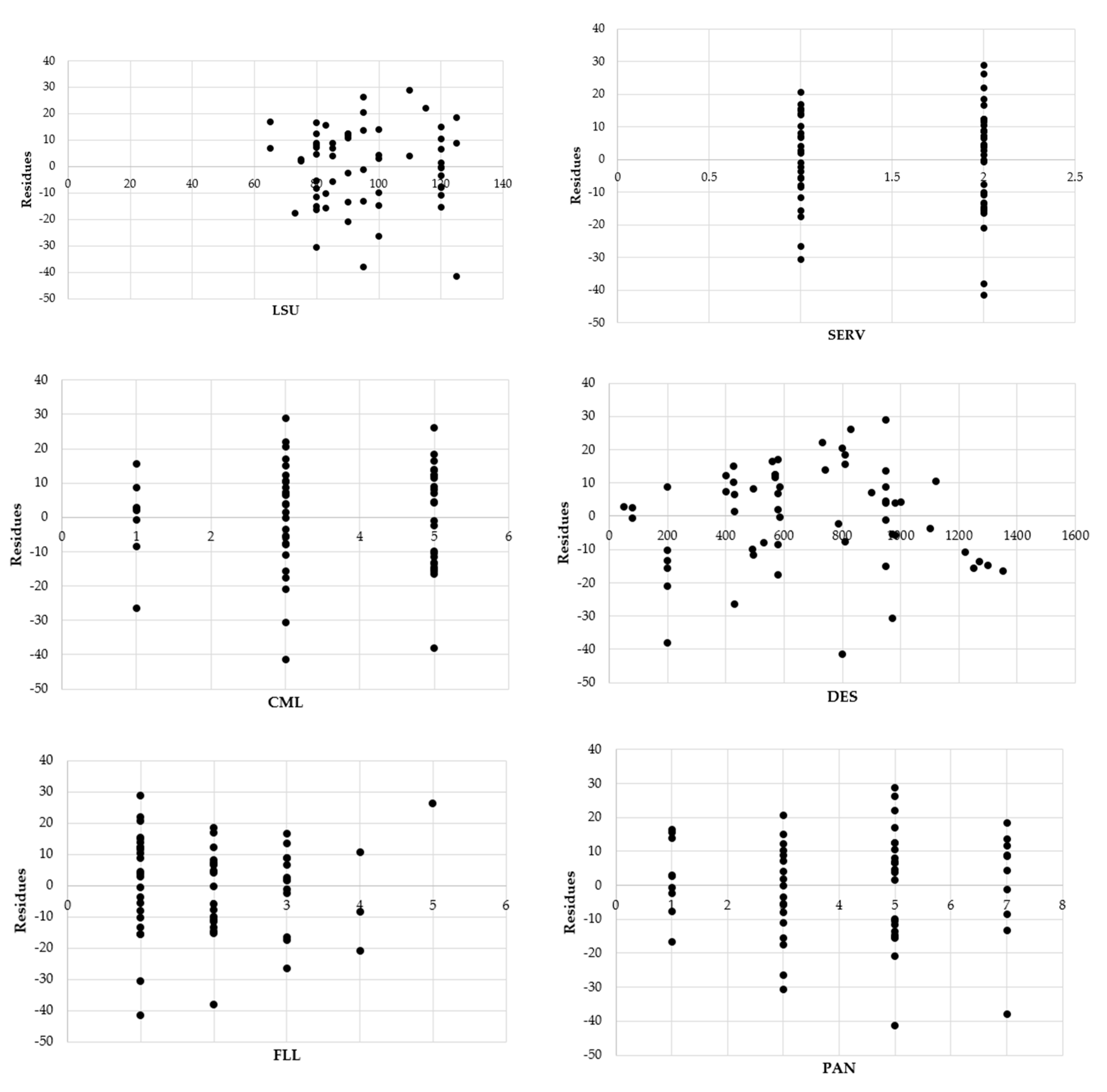
• The hypothesis of homoschedasticity is verified by analyzing the residues. In fact, with the only exception of the FLL variable, however significant for estimation reasons, the graphs of the residues are presented approximately as points clouds that are arranged randomly within a horizontal band, as shown in the graphs in Figure 3;

Once the adequacy of the regression model has been assessed on the basis of the analysis of the residues, it is possible to check whether there is a significant relationship between the dependent variable P and the set of explanatory variables. This verification is carried out by means of the F-test of global significance. Since there is more than one explanatory variable, the null hypothesis H₀ and the alternative hypothesis H1 must be specified as follows:

• H₀: β₁ = β₂ = β₃ = β₄ = β₅ = β₆ = β₇ = 0 (there is no linear relationship between the dependent variable and the explanatory variables);
• H₁: β_j ≠ 0 (there is a linear relationship between the dependent variable and at least one of the explanatory variables).

The rule is:

• Accept H₁ if F > F_crit, where F_crit is the critical value on the right tail of a distribution F with p and n − p − 1 degrees of freedom;
• Otherwise accept H₀.

Referring to the one-tailed ANOVA table with significance level α = 0.05, we obtain F_crit = 2.20. Since F = 62.192532 > F_crit and furthermore F Significance = 0.00 < α, then it is possible to accept H₁ and conclude that there is a linear relationship between at least one explanatory variable and the price P. Therefore, the global significance test is successful.

At this point it is also necessary to verify the significance of each of the seven explanatory variables of the model. For this purpose, the t-test is carried out on the individual regression coefficients, which is equivalent to ascertaining the contribution of each of the independent variables to the formation of the price. In other words, for each of the individual partial regression coefficients of the variables x_i, the t-test shows whether there is a significant linear relationship between the variable x_i and P. Now the hypotheses are:

• H₀: β_i = 0 (there is no linear relationship between the dependent variable P and the explanatory variable x_i);
• H₁: β_i ≠ 0 (here is a linear relationship between x_i and P).

According to the one and two-tailed ANOVA tables with significance level α, the rule is:

• Accept H₁ if t > t_crit, where t_crit is the critical value;
• Otherwise accept H₀.

In relation to the output generated by the model, it is possible to say that:

• Since t stat > t_crit with α = 0.05 (95%), the variables LSU, DES, PAN and LIFT have significant effects on the purchase price. So, taking into account the amount of the other variables, there is a linear relationship between each of the variables considered and the price P;
• Since t stat > t_crit with α = 0.5 (50%), the variable CML has effects on the price;
• The variables SERV and FLL have no evident effects on the purchase price, because t stat < t_crit for any level of α. However, these variables are taken into account in the analysis for extra-statistical considerations based on the importance from an estimative point of view.

6. Results and Discussions

The elaborations developed in the previous paragraph allow to write the regression law that explains the purchase price P as a function of the seven parameters LSU, SERV, CML, DES, FLL, PAN and LIFT. Taking up the coefficients in Table 3.

This function applies to apartments free from contractual obligations, all forming part of multi-storey buildings with 3–4 floors above ground, and with a surface between 70 and 120 m². All the apartments all within a homogeneous zone, where the extrinsic (zonal) characteristics are the same.

According to (13), the price P of the ordinary real estate unit is € 1820/m², to which are added € 2180 for each bathroom over the first one.

Compared to the three possible states of conservation (mediocre, medium, good), the change from one state to a higher one produces a price increase of € 1560. In addition, the price not only increases by € 340 per floor, but also by € 2780 for each level of panoramicity. This is due to the panoramic views of which the study area favorably benefits.

In addition, the presence of the elevator in the multilevel building where the real estate unit is located, entails a price increase of € 9750.

Above all, in terms of DES distance from the ecosystem disservice, as expected, function (13) highlights that the P price of the house increases by € 80/meter as we move away from the polluting production activity. This, of course, up to a spatial limit beyond which the presence of the foundry does not generate immediately perceptible environmental effects and therefore does not cause reductions in property values. This spatial limit coincides with the perimeter of Figure 1, performed in light of the market values recorded in the survey area.

Therefore, it is possible to estimate the maximum decrease in value to which the ordinary apartment undergoes when passing from the limit of the area of influence (see Figure 2) to the minimum distance from the foundry. In estimative terms, the ordinary apartment is the statistically most frequent one, that is, with an area of 95.5 m², equipped with 2 bathrooms, with a 3-medium conservation level, located on the first floor, with a 5-medium panoramic view, served by a lift. Table 1 shows the maximum distance DES_max (equal to 1,350 m) and the minimum distance DES_min (50 m) that the ordinary house can have from the foundry. Therefore, by applying function (12), we obtain that the market value of the property drops from € 241,754 to € 137,953, with a contraction of 42.9%.

This is an extremely important result, which shows how significant the impact of the ecosystem disservice on the real estate values can be.

7. Conclusions

The environmental issue is of primary importance today. The intimate relationship between man and nature, between the urban ecosystem and the natural ecosystem pays attention to the real cause of the environmental disaster, namely the harassing exploitation of the nature.

Addressing the issue on an urban scale means promoting interventions for ecosystem services. The experts of the Millennium Ecosystem Assessment (MEA) identify four different types of services, all fundamental for human well-being and health: provisioning, regulating, cultural and supporting. These are services often overlooked because many of them, as they are not traded on the market, do not have a price that is indicative of their social value.

This study investigates effects that an ecosystem disservice generates on the city. In particular, the calculations concern the estimate of the contraction that the market values of the houses suffer due to the polluting emissions produced by a medium-sized foundry. To solve the valuation problem, multiple regression analysis is used, with the aim of constructing a function capable of explaining the purchase price P of the apartment through multiple variables, one of which is representative of the ecosystem disservice. The variables selected are precisely: living space, number of services provided, state of conservation and maintenance, distance from ecosystem disservice, floor level, panoramic level, and presence of the lift.

This allows to characterize an interpretative and forecasting model of the phenomenon, from which we also deduce the perimeter of the area in which the buildings undergo depreciation due to polluting industrial activities. But above all, the model estimates the implicit marginal prices, i.e., the marginal contribution to the total price for each characteristic, and it shows that the contractions of real estate value can reach 43%. These are extremely important results which, with reference to a medium-sized city (Salerno, Italy), for the first time lead to estimate in quantitative terms the impact of an ecosystem disservice on real estate assets.

The implementation of the model proposed in different urban contexts outlines interesting research perspectives. But already now the model justifies urban planning strategies, and more generally of economic Policy, aimed at minimizing the environmental impacts of human production activities. Also in relation to the direct economic implications related to the decrease in value of the real estate assets.

References

- Farber, S.C.; Costanza, R.; Wilson, M.A. Economic and ecological concepts for valuing ecosystem services. Ecol. Econ. 2002, 41, 375–392. [Google Scholar] [CrossRef]
- UN. MEA Ecosystems and Human Well-being: Multiscale Assessment. Millennium Ecosystem Assessment Series; UN: Washington, DC, USA, 2006. [Google Scholar]
- Costanza, R.; d’Arge, R.; de Groot, R.; Farber, S.; Grasso, M.; Hannon, B.; Limburg, K.; Naeem, S.; O’Nell, R.V.; Paruelo, J.; et al. The value of the world’s ecosystem services and natural capital. Nature 1997, 387, 253–260. [Google Scholar] [CrossRef]
- Daily, G.C.; Soderquist, T.; Aniyar, S.; Arrow, K.; Dasgupta, P.; Ehrlich, P.R.; Folke, C.; Jansson, A.M.; Jansson, B.O.; Kautsky, N.; et al. The value of nature and the nature of value. Science 2000, 289, 395–396. [Google Scholar] [CrossRef] [PubMed] [Green Version]
- De Groot, R.S.; Wilson, M.A.; Boumans, R.M.J. A typology for the classification, description and valuation of ecosystem functions, goods and services. Special Issue: The Dynamics and Value of Ecosystem Services: Integrating Economic and Ecological Perspectives. Ecol. Econ. 2002, 41, 393–408. [Google Scholar] [CrossRef] [Green Version]
- Nesticò, A.; Guarini, M.R.; Morano, P.; Sica, F. An Economic Analysis Algorithm for Urban Forestry Projects. Sustainability 2019, 11, 314. [Google Scholar] [CrossRef] [Green Version]
- Nesticò, A.; Maselli, G. Sustainability indicators for the economic evaluation of tourism investments on islands. J. Clean. Prod. 2020, 248, 119217. [Google Scholar] [CrossRef]
- Del Giudice, V. L’analisi di Regressione Multipla Nella Stima per Valori Tipici, Ce.S.E.T. Seminari. Aspetti Evolutivi Della Scienza Estimativa. Seminario in Onore di Ernesto Marenghi; Firenze University Press: Firenze, Italy, 1995. [Google Scholar]
- Schimmenti, E.; Asciuto, A.; Mandanici, S.; Viviano, P. L’utilizzo della regressione multipla nelle indagini estimative condotte in mercati fondiari attivi: Il caso studio di oliveti e vigneti in un territorio siciliano. Aestimum. Apprais. Rural. Econ. 2012, 60, 53–84. [Google Scholar] [CrossRef]
- Isakson, H.R. Using Multiple Regression Analysis in Real Estate Appraisal. Apprais. J. 2001, 69, 424–430. [Google Scholar]
- Zheng, S.; Cao, J.; Kahn, M.E.; Sun, C. Real Estate Valuation and Cross-Boundary Air Pollution Externalities: Evidence from Chinese Cities. J. Real Estate Financ. Econ. 2013, 48, 398–414. [Google Scholar] [CrossRef]
- Liebelt, V.; Bartke, S.; Schwarz, N. Urban Green Spaces and Housing Prices: An Alternative Perspective. Sustainability 2019, 11, 3707. [Google Scholar] [CrossRef] [Green Version]
- Xu, L.; You, H.; Li, D.; Yu, K. Urban green spaces, their spatial pattern, and ecosystem service value: The case of Beijing. Habitat Int. 2016, 56, 84–95. [Google Scholar] [CrossRef]
- Isaac, D.; O’Leary, J. Property Valuation Principles, 2nd ed.; Palgrave MacMillan: London, UK, 2012. [Google Scholar]
- Kruskal, W.H.; Tanur, J.M. Linear Hypotheses. International Encyclopedia of Statistics; Free Press, Collier Macmillan: London, UK, 1978. [Google Scholar]
- Lindley, D.V. Regression and Correlation Analysis. In Series and Statistics; Eatwell, J., Milgate, M., Newman, P., Eds.; Time Palgrave MacMillan: London, UK, 1990. [Google Scholar]
- Birkes, D.; Dodge, Y. Alternative Methods of Regression; Yohn Wiley Sons: Hoboken, NJ, USA, 2011. [Google Scholar]
- Morano, P. L’analisi di Regressione per le Valutazioni di Ordine Estimativo; Celid: Torino, Italy, 2002. [Google Scholar]
- Acciani, C. La Regressione Lineare Multipla Nelle Valutazioni Immobiliari; Edagricole: Bologna, Italy, 1996. [Google Scholar]
- Bencardino, M.; Nesticò, A. Demographic Changes and Real Estate Values. A Quantitative Model for Analyzing the Urban-Rural Linkages. Sustainability 2017, 9, 536. [Google Scholar] [CrossRef] [Green Version]
- De Luca, A. Le Applicazioni dei Metodi Statistici alle Analisi di Mercato. Manuale di Ricerche per il Marketing; FrancoAngeli: Milano, Italy, 2006. [Google Scholar]
- Damodar, N. Gujarati Essentials of Econometrics; McGraw-Hill Education: New York, NY, USA, 2009. [Google Scholar]
- Stock, J.H.; Watson, M.W. Introduzione All’econometria; Pearson: Torino, Italy, 2005. [Google Scholar]
- Gorla, M.S. Elementi di Statistica Applicata; Maggioli Editore: Rimini, Italy, 2011. [Google Scholar]
- Sen, A.; Srivastava, M. Regression Analysis: Theory, Methods and Applications; Springer: New York, NY, USA, 1990. [Google Scholar]
- Faraway, J. Linear Models with R; CRC Press: Boca Raton, FL, USA, 2004. [Google Scholar]
- Dobson, A.J.; Barnett, A.G. An Introduction to Generalized Linear Models, 3rd ed.; CRC Press: New York, NY, USA, 2008. [Google Scholar]
- Levine, M.D.; Krehbiel, T.C.; Berenson, M.L. Statistica; Apogeo editore: Milano, Italy, 2006. [Google Scholar]
- Morano, P. Un modello di regressione in presenza di outlier per l’analisi del mercato immobiliare. Estimo E Territ. 2001, 10, 19–35. [Google Scholar]
- Micelli, E. Qualità e Valori Immobiliari; Edagricole: Bologna, Italy, 1998. [Google Scholar]
- Agenzia del Territorio Manuale Operativo delle Stime Immobiliari; Agenzia del Territorio: Milano, Italy, 2012.
- De Mare, G.; Nesticò, A.; Tajani, F. The Rational Quantification of Social Housing. An Operative Research Model. ICCSA 2012, 7334, 27–43. [Google Scholar] [CrossRef]
- Epley, D.R.; Burns, W. The Correct use of Confidence Intervals and Regression Analysis in Determining the Value of Residential Homes. Real Estate Econ. 1978, 6, 70–85. [Google Scholar] [CrossRef]
- Waltl, S.R. Variation across Price Segments and Locations: A Comprehensive Quantile Regression Analysis of the Sydney Housing Market. Real Estate Econ. 2016, 47, 723–756. [Google Scholar] [CrossRef]
- Kim, H.; Hung, K.; Park, S.Y. Determinants of Housing Prices in Hong Kong: A Box-Cox Quantile Regression Approach. J. Real Estate Finan. Econ. 2015, 50, 270–287. [Google Scholar] [CrossRef]
- Zietz, J.; Zietz, E.N.; Sirmans, G.S. Determinants of House Prices: A Quantile Regression Approach. J. Real Estate Financ. Econ. 2008, 37, 317–333. [Google Scholar] [CrossRef]
- Rosen, S. Hedonic prices and implicit markets: Product differentiation in pure competition. J. Political Econ. 1974, 82, 34–55. [Google Scholar] [CrossRef]
- Witte, A.D.; Sumka, H.J.; Erekson, H. An Estimate of a Structural Hedonic Price Model of the Housing Market: An Application of Rosen’s Theory of Implicit Markets. Econometrica 1979, 47, 1151–1173. [Google Scholar] [CrossRef] [Green Version]
- Smith, T.R. Multiple regression and the appraisal of single residential properties. Apprais. J. 1971, 39, 277–284. [Google Scholar]
- Smith, B.A. Measuring the Value of Urban Amenities. J. Urban Econ. 1978, 5, 370–387. [Google Scholar] [CrossRef]
- Cohen, J.P.; Coughlin, C.C.; Clapp, J.M. Local Polynomial Regressions versus OLS for Generating Location Value Estimates. J. Real Estate Finan. Econ. 2017, 54, 365–385. [Google Scholar] [CrossRef]
- Simonotti, M. La Stima Immobiliare; UTET Libreria: Milano, Italy, 1997. [Google Scholar]
- Lindley, D.V. Regression and correlation analysis. In New Palgrave: A Dictionary of Economics; Mcmillan: New York, NY, USA, 1987. [Google Scholar]
- Simonotti, M. Un’applicazione Dell’analisi di Regressione Multipla Nella Stima di Appartamenti Genio Rurale; Edagricole: Bologna, Italy, 1991. [Google Scholar]
- Del Giudice, V. L’analisi di regressione multipla nella stima per valori tipici. Aestimum 2009, 15, 119–128. [Google Scholar] [CrossRef]
- Pavlov, A.D. Space-Varying Regression Coefficients: A Semi-parametric Approach Applied to Real Estate Markets. Real Estate Econ. 2003, 28, 249–283. [Google Scholar] [CrossRef]
- Lai, T.-Y.; Wang, K. Comparing the Accuracy of the Minimum-Variance Grid Method to Multiple Regression in Appraised Value Estimates. Real Estate Econ. 1996, 24, 531–549. [Google Scholar] [CrossRef]
- Antoniucci, V.; Marella, G. Small town resilience: Housing market crisis and urban density in Italy. Land Use Policy 2016, 59, 580–588. [Google Scholar] [CrossRef]
- Antoniucci, V.; Marella, G. Is social polarization related to urban density? Evidence from the Italian housing market. Landsc. Urban Plan. 2018, 177, 340–349. [Google Scholar] [CrossRef]
- Dolores, L.; Macchiaroli, M.; De Mare, G. Soglie monetarie per la vendita pubblica di spazi pubblicitari nel contratto di sponsorizzazione culturale. LaborEst 2019, 19, 5–9. [Google Scholar] [CrossRef]
- Nesticò, A.; Maselli, G. Declining discount rate estimate in the long-term economic evaluation of environmental projects. J. Environ. Account. Manag. 2020, 8, 93–110. [Google Scholar] [CrossRef]
- Ross, S.M. Introduzione alla statistica. Maggioli Editore: Rimini, Italy, 2014. [Google Scholar]
Figure 1.
Cartography of the study area.
Figure 2.
Path of the conditioned distributions.
Figure 3.
Analysis of the residues for the independent variables.