Article

Renewable Energy Green Innovation, Fossil Energy Consumption, and Air Pollution—Spatial Empirical Analysis Based on China

1
College of Public Administration, Huazhong University of Science and Technology, Wuhan 430074, China
2
School of Economics and Management, Fuzhou University, Fuzhou 350108, China
3
School of Management, Huazhong University of Science and Technology, Wuhan 430074, China
4
Business College, Guilin University of Technology, Guilin 532100, China
*
Author to whom correspondence should be addressed.
Sustainability 2020, 12(16), 6397; https://0-doi-org.brum.beds.ac.uk/10.3390/su12166397
Submission received: 4 July 2020 / Revised: 1 August 2020 / Accepted: 4 August 2020 / Published: 8 August 2020
(This article belongs to the Section Energy Sustainability)

Abstract

:
Excessive consumption of traditional fossil energy has led to more serious global air pollution. This article incorporates renewable energy green innovation (REGI), fossil energy consumption (FEC), and air pollution into a unified analysis framework. Using China’s provincial panel data, a spatial measurement model was used to investigate the spatial effects of renewable energy green innovation and fossil energy consumption on air pollution in China from 2011 to 2017. The global Moran index shows that over time, the spatial correlation of air pollution has gradually weakened, while the global correlation of renewable energy green innovation and fossil energy consumption is increasing year by year. ArcGIS visualization and partial Moran index show that air pollution, renewable energy green innovation, and fossil energy consumption are extremely uneven in geographic space. The spatial distribution of air pollution, renewable energy green innovations, and fossil energy consumption are all characterized by high in the east and low in the west and they all show a strong spatial aggregation. Applying the spatial adjacency matrix to the spatial Durbin model gave the results that China’s air pollution has a significant spatial spillover effect. Replacing fossil fuels with clean renewable energy will reduce air pollutant emissions. The Environment Kuznets Curve (EKC) hypothesis has not been supported and verified in China. The partial differential method test found that the spatial spillover benefits can be decomposed into direct effects and indirect effects. The direct and indirect effects of renewable energy green innovation on air pollution are both significantly negative, indicating that green innovation of renewable energy not only inhibits local air pollution, but also inhibits air pollution in nearby areas. The consumption of fossil energy will significantly increase the local air pollution, while the impact of sulfur dioxide (SO2) and soot (DS) pollution in nearby areas is not obvious. It is recommended to increase investment in renewable energy green innovation, reduce the proportion of traditional fossil energy consumption, and pay attention to the spatial connection and overflow of renewable energy green innovation and air pollution.

1. Introduction

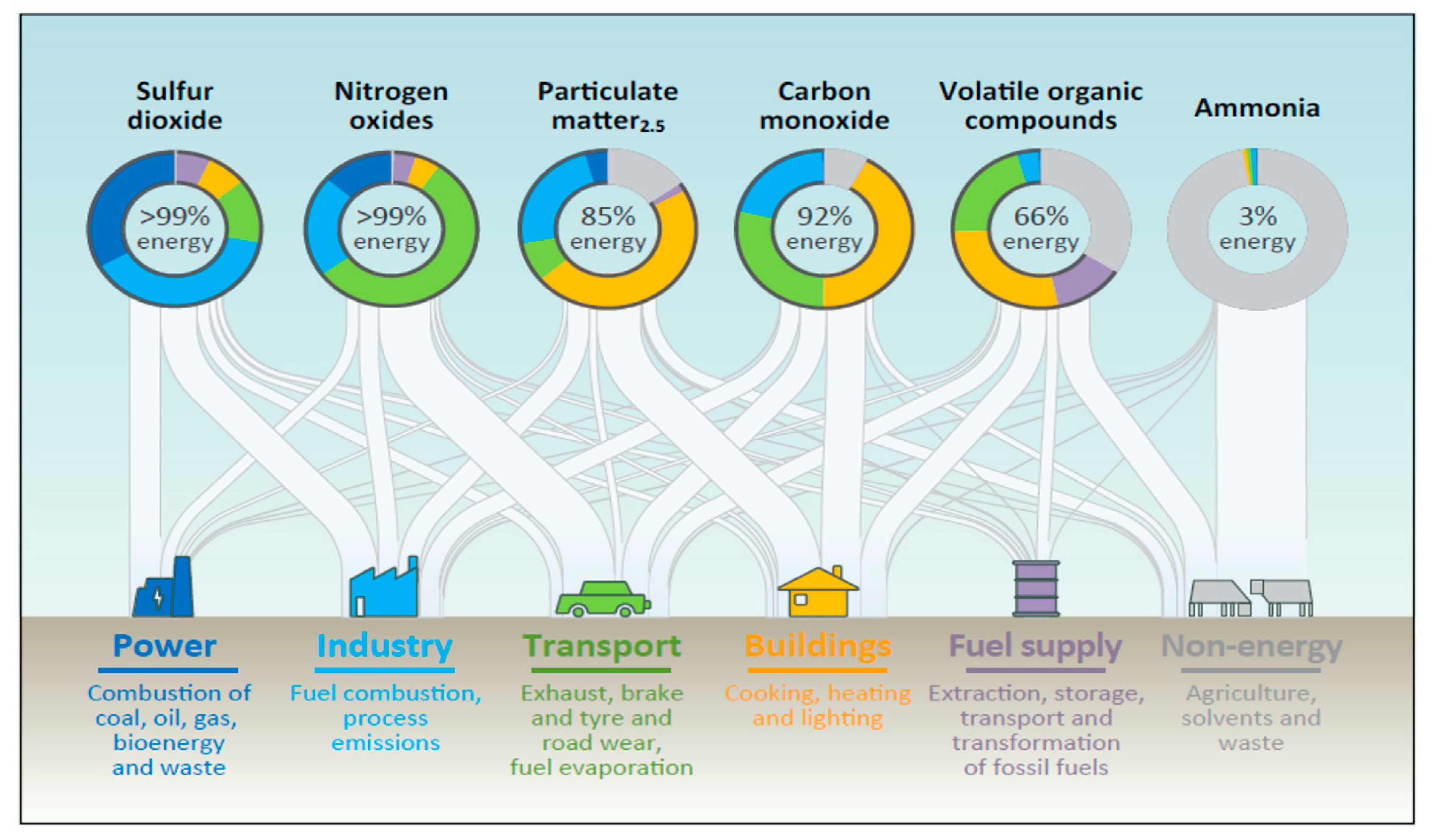
In the 21st century, with the rapid economic development, China’s energy consumption has been rising rapidly. As a result of the massive increase in energy consumption, the air pollution problem has become more serious. According to a report by the International Energy Agency [1], as shown in Figure 1, up to 99% of sulfur dioxide (SO2) and oxynitride (NOx) emissions and up to 85% of fine particulate matter (PM2.5) emissions are attributable to energy production and use [1].
The sulfur dioxide (SO2), nitrogen oxides (NOx), and soot (DS) in China’s air pollutants mainly come from the burning of fossil fuels. In China’s fossil energy consumption, coal is the most important energy source. Therefore, an important cause of air pollution in China is the burning of coal as a fuel [2]. Coal combustion produces a large amount of SO2, NOx, DS, which increases the concentration of air pollutants. Studies have shown that an increase in the concentration of air pollutants will significantly reduce the health of residents [3]. Both short-term and long-term income elasticity show that sulfur oxide emissions have a significant positive impact on health expenditures [4]. Moreover, previous studies have found that air pollution has a strong spatial spillover effect, and air pollution has a strong mutual influence in geographically similar cities or regions [5,6,7,8].
Therefore, to reduce air pollution, it is necessary to reduce the proportion of coal consumption in fossil energy consumption, and thus the SO2, NOx, and DS emissions during the energy consumption process are reduced. At this stage, to reduce the proportion of coal consumption, replacing fossil fuel combustion with clean renewable energy is generally considered to be the best solution [9]. Therefore, increasing the proportion of renewable energy consumption to replace part of the fossil energy consumption is a very suitable solution to the problem of air pollution. However, the problem is that the price, stability, and technological maturity of renewable energy at this stage are worse than those of fossil energy. Obviously, this hinders the consumption of renewable energy. Therefore, if we want to increase the proportion of renewable energy consumption on the consumer side, we must strengthen the green innovation of renewable energy. When the price, stability, and technological maturity of renewable energy are comparable to fossil energy, the proportion of renewable energy consumption will increase. As a result, the proportion of coal consumption will drop, and the air pollution problem will be alleviated.
However, existing research focuses on the impact of energy consumption and economic and social factors on air pollutant emissions. Some scientists have separately studied the impact of renewable energy green innovation on air pollution and the impact of fossil energy consumption on air pollution. However, there are not many scientists who have combined renewable energy green innovation and fossil energy consumption to conduct research. Among researchers, spatial effects have not received enough attention.
To improve the research in this area, this article fully considers the spatial effect. Using spatial econometric models, we investigated the temporal and spatial evolution characteristics, spatial correlation, and spatial aggregation effects of air pollution in China. This article also focuses on the impact of renewable energy green innovation and fossil energy consumption on air pollution emissions.
The rest of this research is organized as follows. Section 2 is a literature review of related research and the contributions of this research. Section 3 introduces the variables, models, data sources, and methods of this study. Section 4 presents the results and discussion of spatial exploration analysis. Section 5 shows the empirical results of the spatial panel model. Conclusions and policy recommendations can be found in Section 6.

2. Literature Review

In recent years, the increasing energy consumption and increasingly unreasonable energy consumption structure have aggravated the air pollution problem, attracting the attention of many scientists [10,11,12].
Among the influencing factors of air pollution, fossil energy consumption is an important incentive [13,14,15]. Research shows that 75% of global greenhouse gas emissions, 66% of nitrogen oxide emissions, and most of the emissions of particulate matter (PM2.5) come from the energy sector [16] with oil, coal, and natural gas energy as the main energy consumption resources. Coal consumption has become the main type of energy consumption in the industrial sector and thermal power plants [17]. Considering the situation, China relies on thermal power generation, and thermal power plants emit a large amount of SO2 and NOx, which are considered to be the main reason for China’s sulfur dioxide emissions [18]. Electricity consumption is also considered as non-clean energy consumption [19]. Zhang, S. et al. (2015) [20] found that the cement industry is China’s second-largest energy-consuming industry and the main source of carbon dioxide and air pollutants. The cement industry accounts for 7% of China’s total energy consumption and 15% of CO2, accounting for 21% of PM, 4% of SO2, and 10% of NOx. Kanada et al. (2013) [21] found that the consumption of energy fossils is an important source of SO2 in major cities. Yuan, J. et al. (2017) [22] found that due to the large-scale utilization of high-carbon fossil energy, many critical air pollutants (CAPs) and greenhouse gases (GHGs) are emitted, which has led to increasingly serious problems of global climate change and local air pollution.
The renewable energy green innovation that this article focuses on is considered to play an important role in alleviating air pollution [23,24]. This is because the green innovation of renewable energy can promote the consumption and application of clean and renewable energy, replace fossil energy, and reduce air pollution [25]. Boudri, J. et al. (2002) [26] studied the potential of China and India in using renewable energy and their cost-effectiveness in reducing air pollution in Asia. It is found that increasing the use of renewable energy can reduce the cost of controlling sulfur dioxide emission by 17%–35% in China, and reduce the cost of controlling sulfur dioxide emission by more than two-thirds in India. Alvarez et al. (2017) [27] confirmed the positive impact of the energy innovation process on air pollution and pointed out that renewable energy can help improve air quality. Xie et al. (2018) [28] concluded through scenario analysis that improvements in renewable energy have always been more effective than taxation in reducing carbon dioxide and air pollutant emissions. Zhu et al. (2019) [29] found that technological innovations in renewable energy help reduce the concentration of nitrogen oxides (NOx) and respirable suspended particulates (PM10). Obviously, increasing the proportion of clean energy consumption and reducing fossil energy consumption are very effective ways to control air pollution and achieve green development [24,30].
Most of the previous literature separately studied the impact of fossil energy consumption or renewable energy green innovation on air pollution. Previous scientists rarely integrated renewable energy green innovation and fossil energy consumption to study their impact on air pollution. There are not many scientists studying the alternative relationship between fossil energy consumption and renewable energy. There is not enough attention on the spatial correlation and spatial overflow between the three. However, as small as individual cities, as large as individual provinces or regions, the discharge of pollutants has spatial spillover and correlation effects. Xie et al. (2019) [21] found that PM2.5 pollutants have strong spatial spillover characteristics. Zhao et al. (2018) [31] discussed the temporal trends and spatial differences of air pollution in five hotspots in China, as well as the impact of macro-influencing factors on four pollutants, and found that there is a spatial spillover phenomenon of particulate matter across the country. Zeng, et al. (2019) [32] found that provincial renewable energy policies have a positive impact on the reduction of SO2 and PM2.5, and that the energy policy of a province will affect the pollutant emissions of neighboring provinces. Li et al. (2020) [33] found that air pollution emissions have a significant agglomeration effect, and the spatial accumulation pattern of air pollution emissions is similar to that of fossil energy consumption. The proportion of clean energy consumption and the allocation of energy and labor factors have suppressed air pollution emissions.
Therefore, this article will fully explore how renewable energy innovation affects air pollution, organically integrate the substitution relationship between renewable energy and fossil energy, and fully consider the spatial spillover and related effects of renewable energy. Furthermore, it will explore the linkage mechanism and interaction relationship among renewable energy green innovation, fossil energy consumption, and air pollution. Specifically, the contribution of this research will lie in the following aspects. First, we use non-spatial models and spatial measurement models to study the impact of renewable energy green innovation and fossil energy consumption on air pollution. Second, we fully consider the spatial correlation and spatial spillover effects of renewable energy green innovation and fossil energy consumption, and quantify their impact on air pollution. Third, we use visualization methods to show the temporal and spatial characteristics of renewable energy green innovation, fossil energy consumption, and air pollution. Fourth, we expand the STIRPAT (stochastic impacts by regression on population, affluence, and technology) model to quantify the impact of renewable energy green innovation, fossil energy consumption, environmental regulations, industrial structure, population, GDP (Gross Domestic Product), and other factors on air pollution.
The framework of this study is shown in Figure 2. Among them, REGI (renewable energy green innovation) has a positive effect on RE (renewable energy). RE has a negative effect on FEC (fossil energy consumption) and AP (air pollution). FEC has a positive effect on AP.

3. Methodology

3.1. Variables and Data

3.1.1. Explained Variable

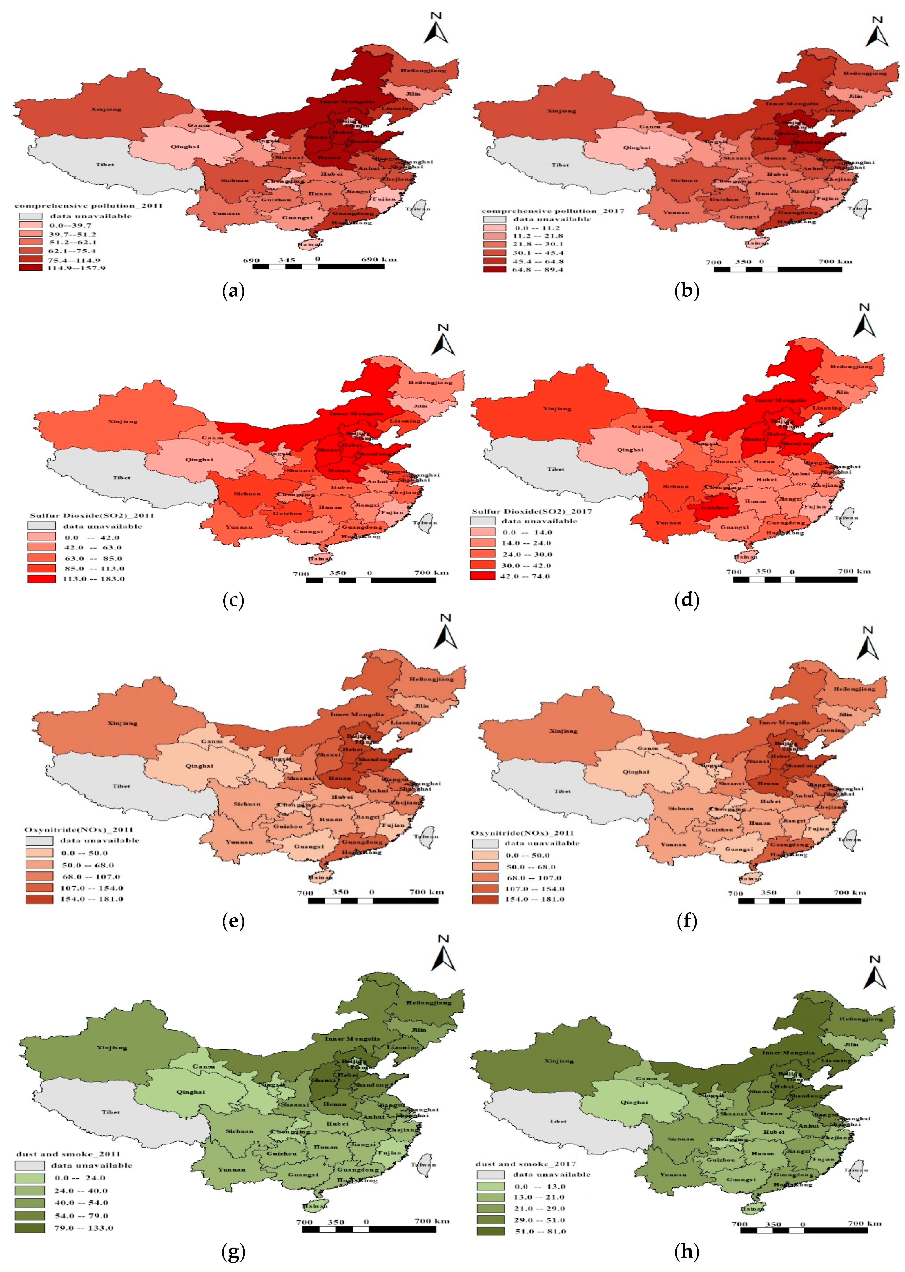
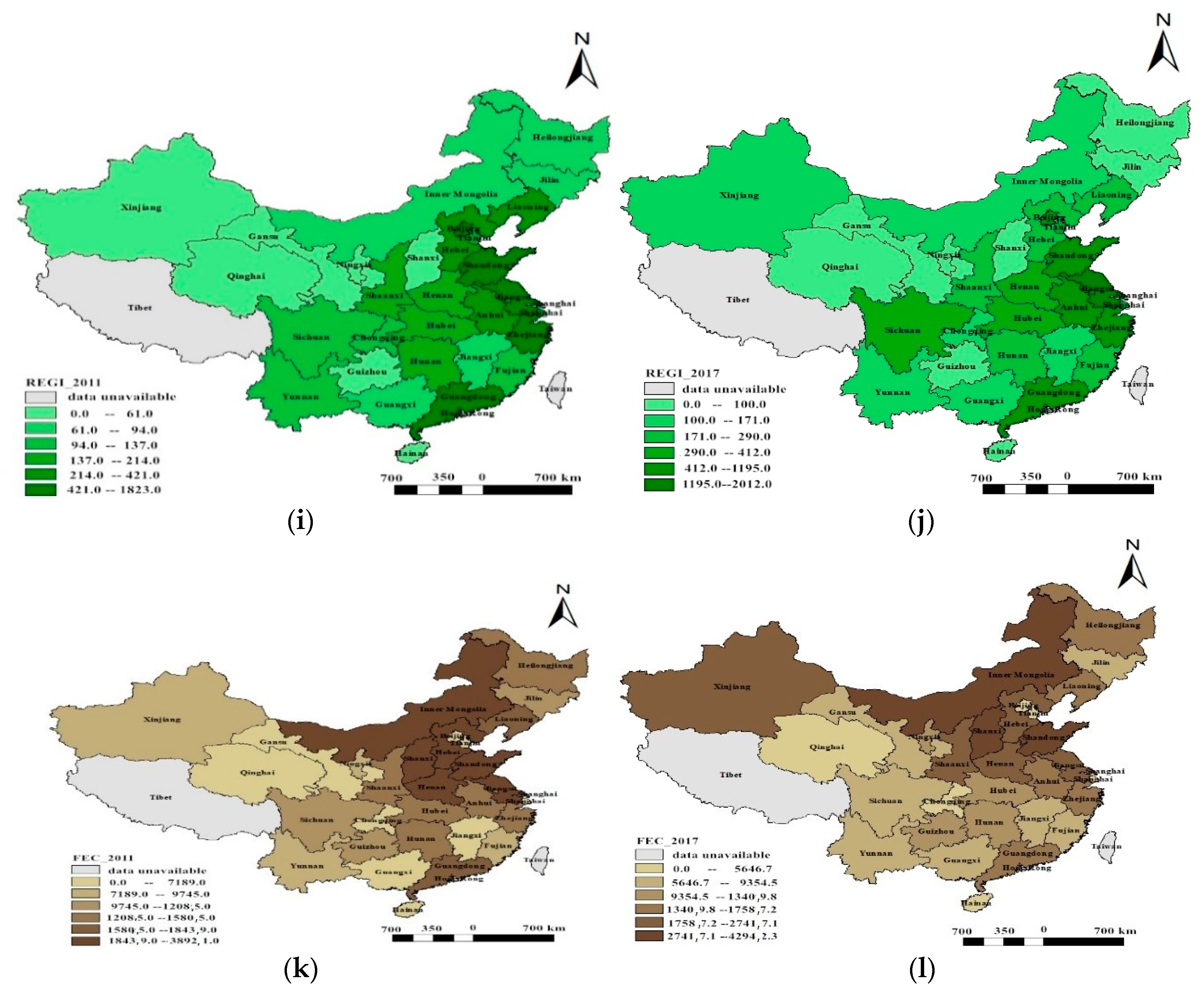
Air pollution: The most representative variable of air pollution is air pollutant emission. In previous studies, the concentration of PM2.5 was generally used as a proxy variable to measure the degree of air pollution. However, PM2.5 cannot make an objective and comprehensive evaluation of air pollution. Therefore, the pollutant indicators for measuring air pollution in this article mainly include sulfur dioxide (SO2), oxynitride (NOx), and dust and smoke (DS). In addition, considering that each pollutant has its own limitations, this article reduces the dimensions of these indicators to obtain a new indicator—comprehensive pollution (CP). Consequently, an objective and comprehensive assessment of air pollution is made.
This article draws on the method of Liu et al. (2015) [34] for index dimensionality reduction. First, the three environmental output indicators are subjected to a unified dimensionality reduction process by factor analysis. After the Bartlett sphere test, the statistic value is 56.077, the significance probability is 0.000, and the Kaiser–Meyer–Olkin (KMO) value is 0.748. Therefore, the null hypothesis that the indicators are not correlated is rejected. It is suitable for factor analysis. At the same time, the corresponding weight of each indicator is calculated through the factor score matrix and the variance contribution rate of the common factor. As a result, the weights of sulfur dioxide, nitrogen oxides, and dust and smoke indicators were 24%, 49%, and 27%, respectively. Combining the weights of the three types of pollution indicators, the comprehensive pollution (CP) can be calculated, and the formula is as follows:
C P i t = i = 1 n w i t X i t
Among them: w i t is the weight of each pollutant, X i t is the pollutant component.

3.1.2. Explanatory Variables

Main Explanatory Variable

(1). Renewable Energy Green Innovation (REGI): The article selects renewable energy patents as a proxy variable for green innovation. Refer to Zhu, Y et al. (2019) [29] to select the International Patent Classification (IPC) code shown as Table 1 to represent the renewable type. The patent has an impact on the corresponding technology from the date of application. Therefore, previous studies mostly counted the number of patents from the date of patent application. This article refers to the practice of Wang ban-ban et al. (2019) [35]; count the number of renewable energy green patents based on the date of application.
Hypothesis 1a.
Renewable energy green innovation will reduce comprehensive pollution (CP) emissions.
Hypothesis 1b.
Renewable energy green innovation will reduce sulfur dioxide (SO2) emissions.
Hypothesis 1c.
Renewable energy green innovation will reduce oxynitride (NOx) emissions.
Hypothesis 1d.
Renewable energy green innovation will reduce dust and smoke (DS) emissions.
(2). Fossil energy consumption (FEC): China’s rapid development has led to a large consumption of energy, especially fossil fuel consumption. The main cause of pollution is the consumption of fossil fuels, and coal consumption accounts for more than 50% of China’s fossil energy consumption [36]. Therefore, coal consumption and pollutant emissions are closely related, so this paper selects coal consumption to represent fossil energy consumption.
Hypothesis 2a.
Fossil energy consumption (FEC) will increase comprehensive pollution (CP) emissions.
Hypothesis 2b.
Fossil energy consumption (FEC) will increase sulfur dioxide (SO2) emissions.
Hypothesis 2c.
Fossil energy consumption (FEC) will increase oxynitride (NOx) emissions.
Hypothesis 2d.
Fossil energy consumption (FEC) will increase dust and smoke (DS) emissions.

Control Variable

(1)
Environmental Regulation (ER): There are many ways to measure the intensity of environmental regulation, considering China’s environmental pollution control policies. This article refers to the practice of Zhu Y et al. (2019) [29] and selects the number of environmental punishment cases as a proxy variable for the intensity of environmental regulation. To a certain extent, environmental regulations will restrain the emission of micro-subjects.
(2)
Industrial Structure (IS): Select the proportion of the secondary industry as a proxy variable. The study of Hao et al. (2016) [37] shows that the correlation coefficient between the proportion of secondary industry and the amount of pollutant emissions is positive. Therefore, this article assumes that there is a positive correlation between industrial structure and air pollution.
(3)
Gross Domestic Product (GDP): Due to the difference between nominal GDP and real GDP, this article is based on the GDP of each province and municipality directly under the central government in 2000. By calculating the GDP deflator, the constant price GDP is calculated.
(4)
Population (POP): There is a direct link between population size and pollutant emissions. An increase in population will significantly increase energy consumption and pollutant emissions.

3.1.3. Variable Descriptive Statistics

The descriptive statistics of all variables in this article are shown in Table 2.

3.1.4. Data Resources

The emission data of air pollutants and the data of environmental regulations come from the China Environmental Yearbook. Energy consumption data comes from China Energy Statistical Yearbook. The GDP and population data come from the China Statistical Yearbook. Patent data comes from the wisdom bud patent database.

3.2. Spatial Autocorrelation Test

3.2.1. Global Correlation Index

Here, this article calculates the global spatial correlation according to the global Moran index:
Moran s   I g l o b a l = i = 1 n j i n w i j ( x i x ¯ ) ( x j x ¯ ) σ 2 i = 1 n j i n w i j = i = 1 n j i n w i j ( x i 1 n i = 1 n x i ) ( x j 1 n i = 1 n x i ) 1 n i = 1 n ( x i 1 n i = 1 n x i ) 2 i = 1 n j i n w i j
Among them: x i ,   x j represent spatial and geographic units i and j, and i ≠ j. w i j represents the spatial weight matrix; x ¯ represents the average value of each province and municipality. σ 2 represents the variance; ( x i x ¯ ) ( x j x ¯ ) represents the similarity between spatial units i and j; n represents the number.

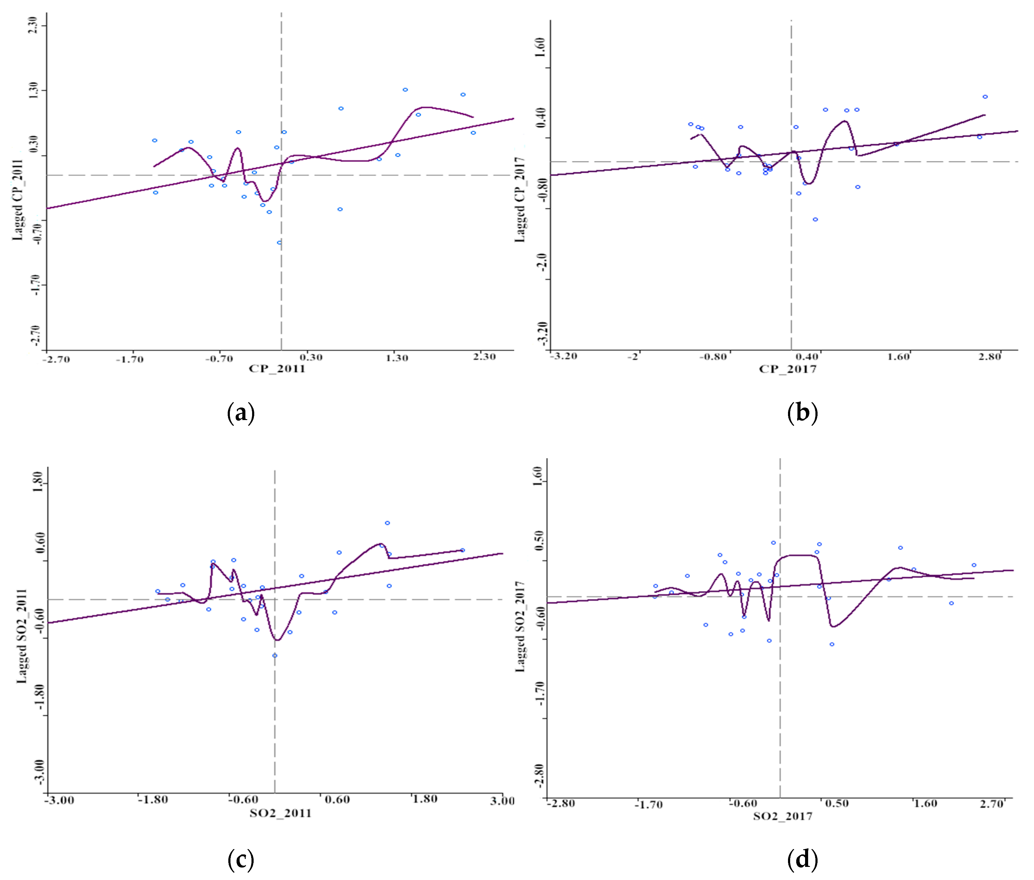
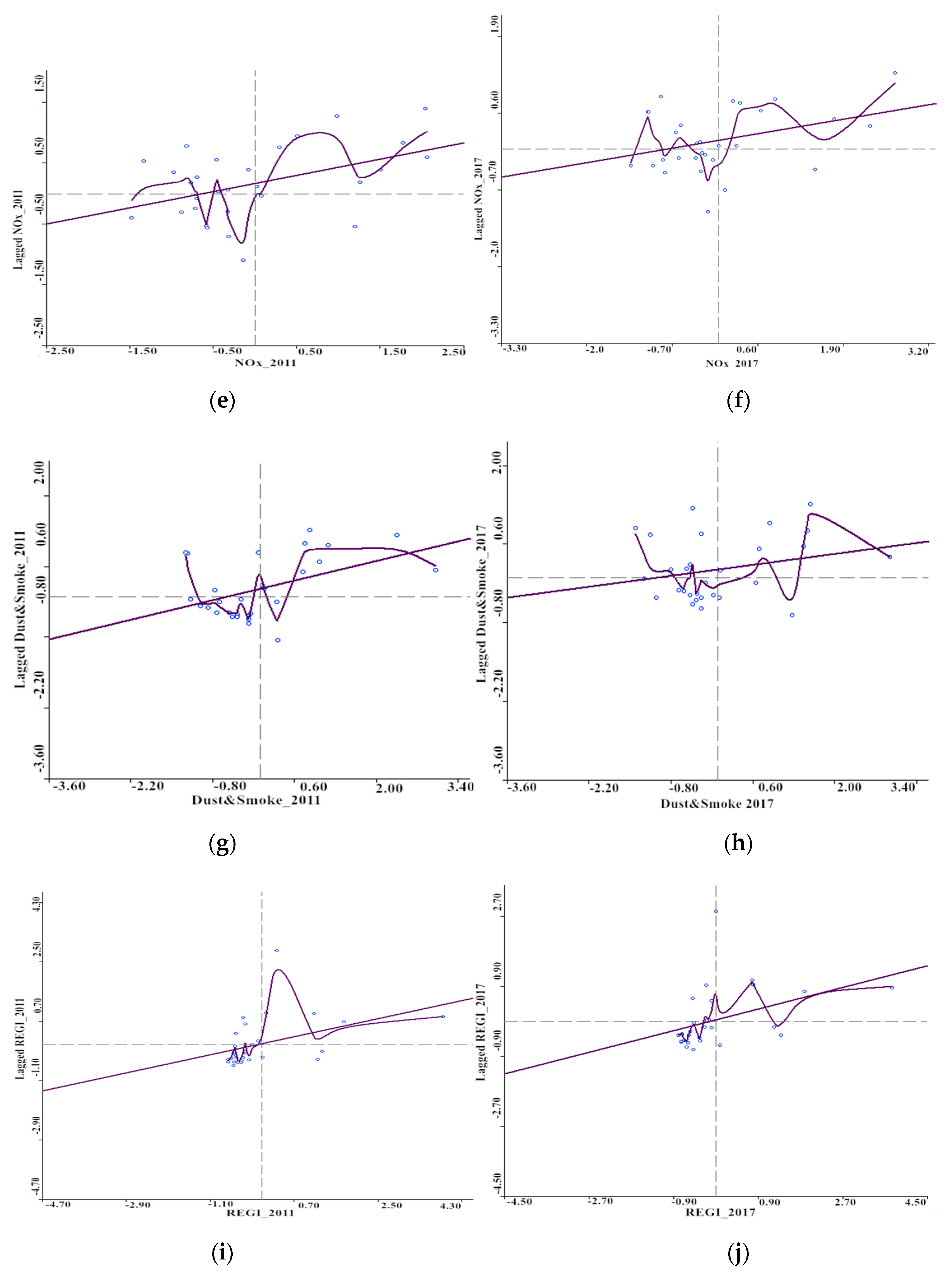
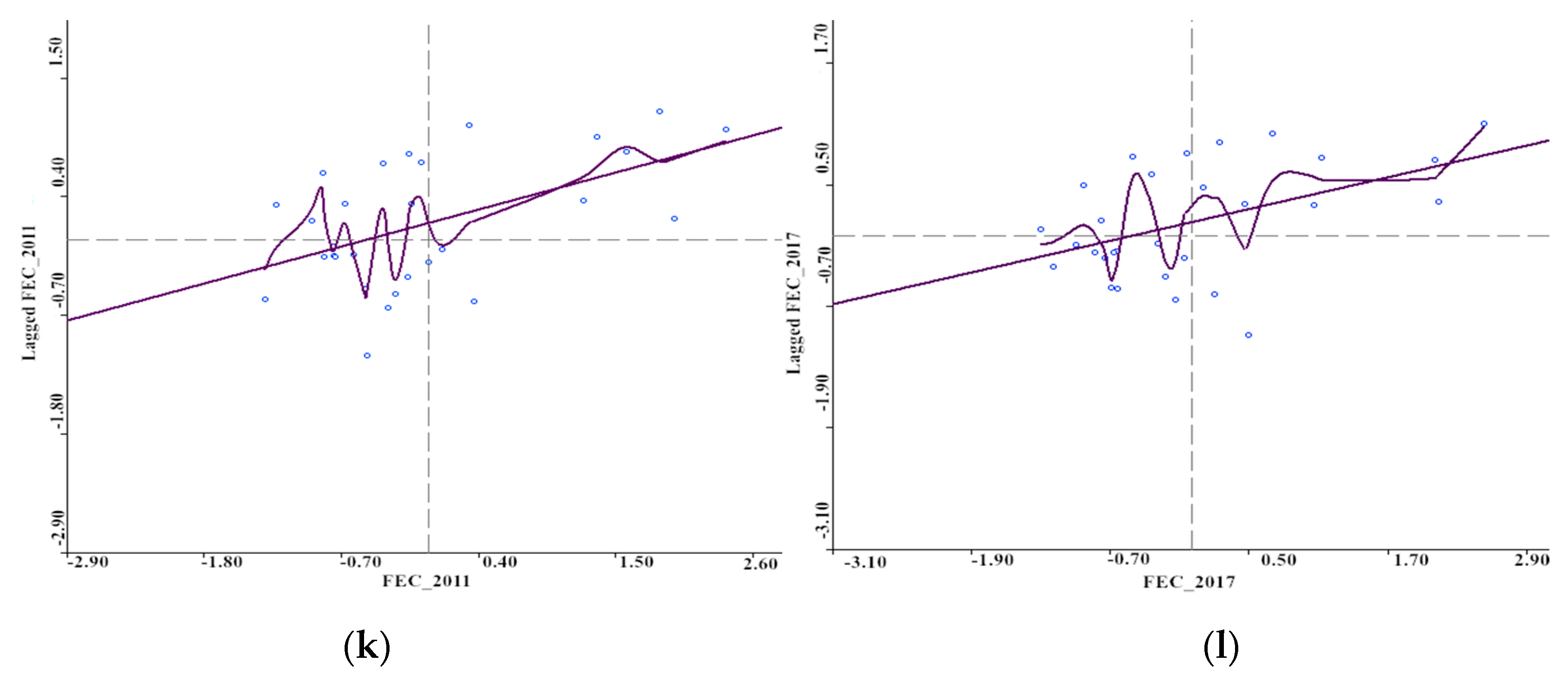
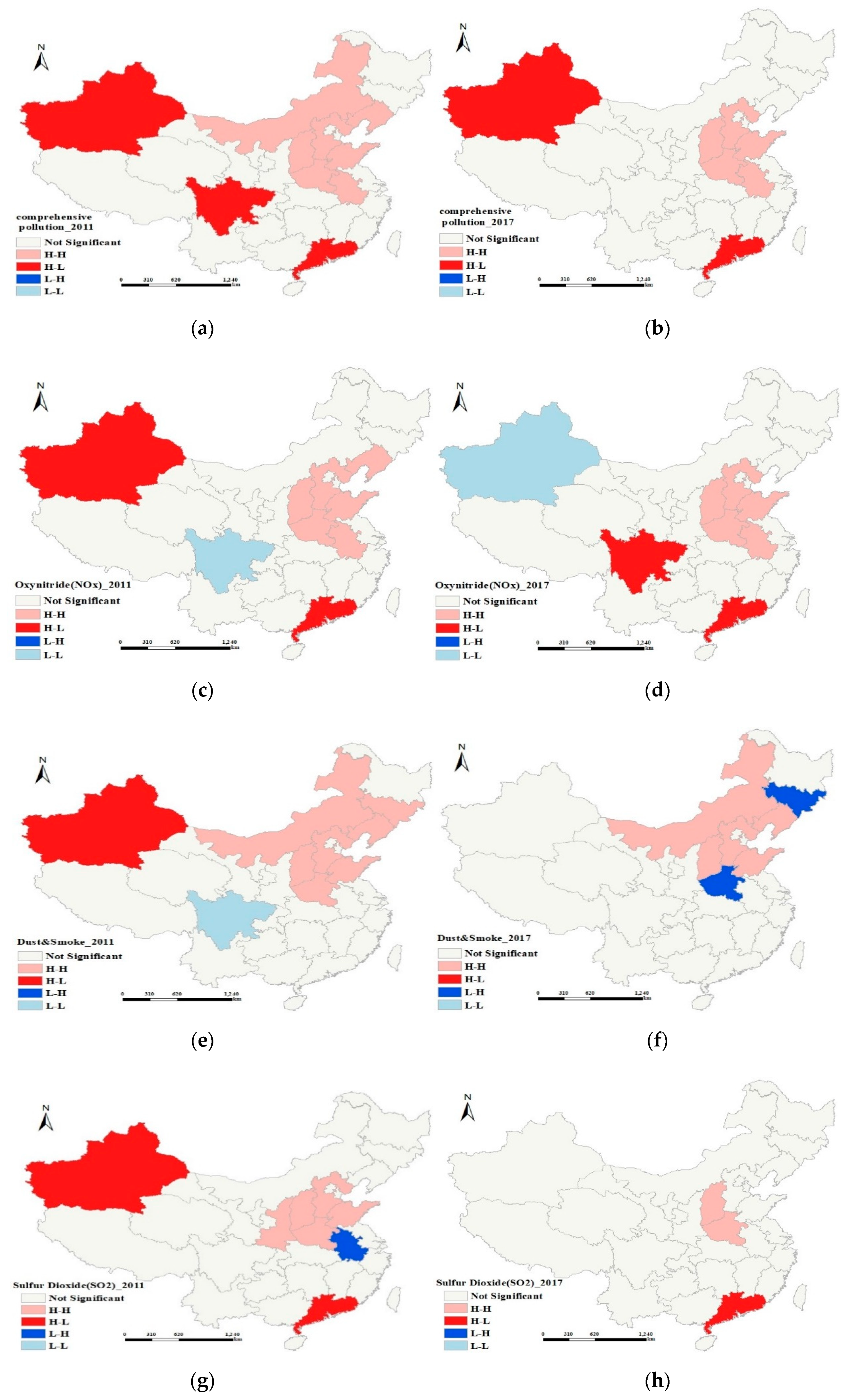
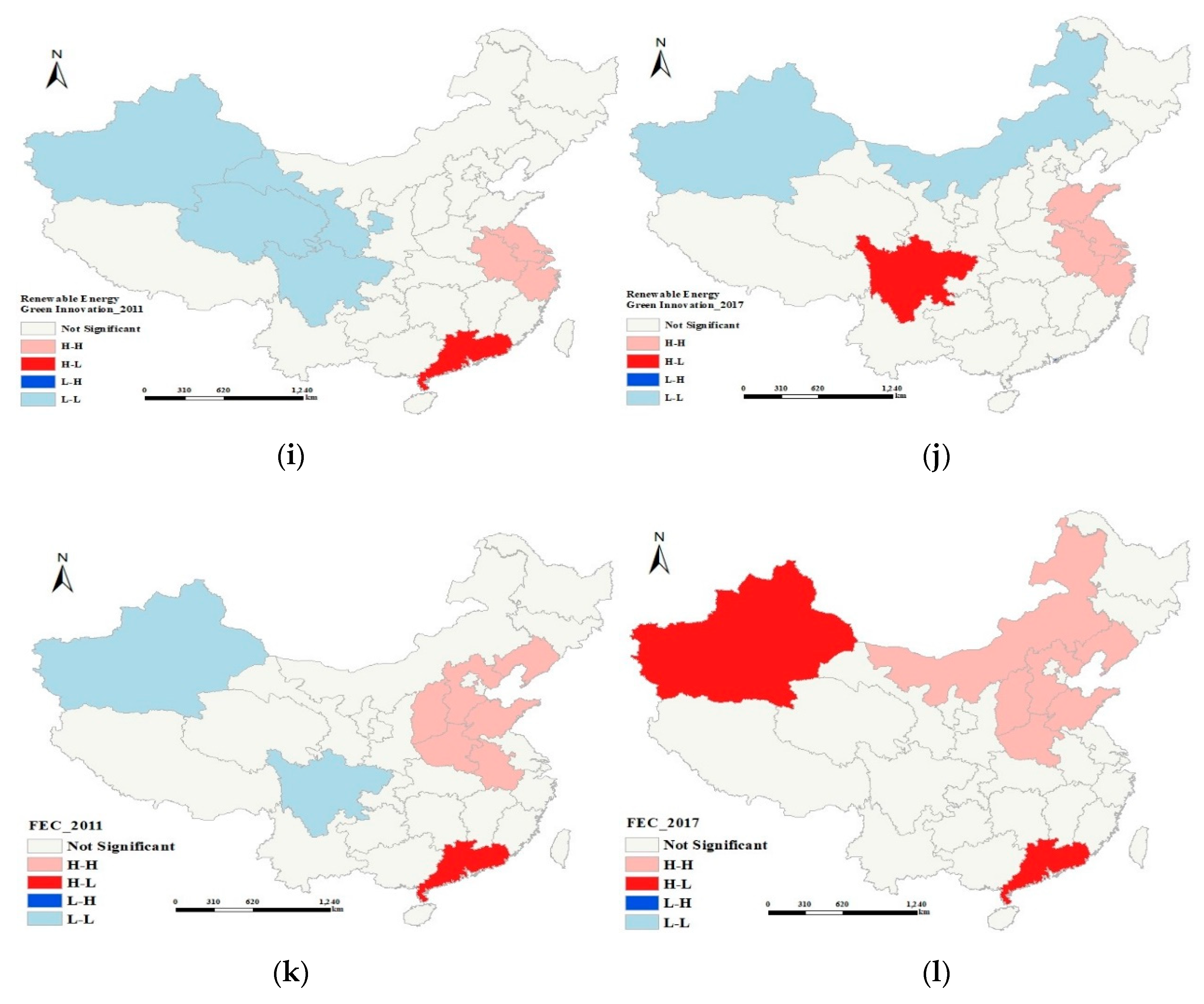
3.2.2. Local Correlation Index

However, the global correlation index cannot measure the local correlation, so the local Moran index needs to be quoted:
Moran s   I i l o c a l = n ( x i x ¯ ) j = 1 n W i j ( x j x ¯ ) i = 1 n ( x i x ¯ ) 2
(1)
H–H: area units with high observation values are surrounded by high-value areas.
(2)
H–L: area units with high observation values are surrounded by areas with low values.
(3)
L–L: area units with low observation values are surrounded by low-value areas.
(4)
L–H: area units with low observation values are surrounded by high-value areas.
Whether it is global spatial autocorrelation or local spatial autocorrelation, the establishment of the spatial weight matrix is very important. This article selects the spatial adjacency weight matrix.
The spatial adjacency weight matrix is a spatial weight matrix that reflects the spatial adjacency relationship. It can be set that there is a significant mutual influence relationship between the adjacent areas, and the non-adjacent areas have no significant interaction. The spatial adjacency weight matrix can more closely reflect the spatial relationship of the development indicators of each region. Therefore, this paper introduces the spatial adjacency weight matrix to make the spatial relationship of development indicators specific.
W i j A = { 1 ,   i f   p r o v i n c e   i   a n d   j   i s   a d j a c e n t 0 ,   i f   p r o v i n c e   i   a n d   j   i s   n o t   a d j a c e n t

3.3. Spatial Econometric Model

Based on the above regression model, we set a general provincial pollutant emission regression model.
The IPAT (Impact, Population, Affluence, Technology) model is used to explore the complex social dynamics generated by environmental problems. The original IPAT model was proposed by the famous American demographers Ehrlich and Holdren in 1971. The model believes that environmental pressure (impact) is the product of population (population), affluence (affluence), and technology (technology) [38]. Dietz et al. (2004) [39,40,41] expressed the IPAT model in a stochastic form to estimate the environmental impact of population, wealth, and technological level. A STIRPAT model (stochastic impacts by regression on population, affluence, and technology) was proposed. The specific expression of the STIRPAT model is:
I i t = a P i t b A i t c T i t d e i t
Among them, a is a constant term; b, c, and d are exponential terms of P, A, and T, respectively; and e is an error term.
Take the logarithm of the left and right sides of the equation:
ln   I i t = l n a + b l n P i t + c l n A i t + d l n T i t + l n e i t
Applied to this article, the following formula can be obtained:
ln   Y i t = λ 0 + λ 1 l n R E T I i t + λ 2 l n P O P i t + λ 3 l n G D P i t + e i t
However, the general regression model does not consider the spatial influence between variables, and the spatial economic model incorporates the spatial influence on the basis of the general regression model [39]. The spatial lag model (SLM) can be expressed as:
y = ρ Wy + X β + ε
where Y is the vector of the dependent variable; X represents an explanatory variable matrix; W is the spatial weight matrix; Wy is the vector of the spatial lagging dependent variable; ρ is the spatial regression coefficient, reflecting the spatial autocorrelation relationship of the dependent variable; β is a parameter vector, reflecting the influence of explanatory variables on dependent variables; and ε is a vector of disturbance terms.
By distinguishing the spatially related error ε and the spatially independent error μ, the spatial error model (SEM) can be expressed as [42]:
{ y = X β + ε ε = λ W ε + μ
Among them, λ is the spatial autocorrelation coefficient on the error term, reflecting the influence of the residual of the nearby area on the residual of the area; μ is the interference term of a vector. The values of other variables and parameters are the same as the SLM formula.
For SLM and SEM, specific panel data estimation methods are used, namely: fixed effects and random effects are calculated in this study. In addition, to estimate the spatial spillover effects of each region, this study examines the direct and indirect effects of explanatory variables.
As a result of the mutual influence among air pollution, innovation factors, and energy factors in different regions. When measuring their influence from a spatial perspective, the spatial measurement model is generally used. For the sake of generality, this article adopts the spatial Durbin model (SDM), which is the general form of the spatial lag model (SLM) and the spatial error model (SEM), and its expression is:
y i t = δ j = 1 n W i j y i t + c + x i t β + j = 1 n W i j x i t θ + μ i + λ t + ε i t
Among them, y i t is the explained variable, x i t is the explanatory variable, c is the constant term, δ is the spatial autoregressive coefficient, β and θ are the coefficients to be estimated, and ε is the residual term. x i t β is the influence of the regional independent variable on the dependent variable. δ j = 1 n W i j y i t is the spatial lag term, which means that the explanatory variable of each spatial unit (i = 1 …, n) is at time t (t = 1 …, T) the dependent variable composed of observations. ε i t is an independent and identically distributed random error term; μ i and λ t represent spatial and temporal effects, respectively. This paper constructs spatial variables: W* dependent variables describe the spatial spillover effects of pollutant emissions, renewable energy green innovation, and fossil energy consumption. W is the spatial weight, which indicates the degree of correlation and mutual influence between various spatial elements.

3.4. Direct and Indirect Spatial Impact

In the spatial econometric model, the independent variable usually has an indirect effect on the dependent variable in the surrounding area (spatial spillover). We estimated direct, indirect, and total spatial effects based on estimated spatial regression coefficients [43,44]. We further quantified the spatial spillover effects of renewable energy green innovation, energy consumption, and other socio-economic indicators on air pollution. Determine the direct and indirect spatial effects according to the determined spatial correlation coefficient ρ, as shown in the formula below:
Y t = ( X t β + W X θ + ε + τ n α t ) I ρ W 1
where X represents the explanatory variable, τ n represents the constant vector, and α is the parameter of the intercept term.
The partial derivative differential equation matrix of the explained variable to the Kth independent variable is:
[ y X ik y X Nk ] = [ y 1 X ik y 1 X nk y n X ik y n X nk ] = ( I ρ W ) 1 [ β k w 21 θ k w n 1 θ k w 12 θ k β k w n 2 θ k w 1 n θ k w 2 n θ k β k ]
The above Equation (12) defines the average value of the sum of the elements of the right matrix as a direct effect. The average value of the sum of all row and column elements of off-diagonal elements is an indirect effect, reflecting the influence of other regional independent variables on regional dependent variables.

4. Exploratory Spatial Analysis Results and Discussion

4.1. Temporal and Spatial Distribution Characteristics of Air Pollution, REGI, and Fossil Energy Consumption

To visually display the spatial and temporal distribution characteristics of comprehensive pollution (CP), SO2, NOx, dust and smoke (DS), renewable energy green innovation (REGI), and fossil energy consumption (FEC) we used ArcGIS to show the spatial and temporal distribution characteristics of China’s 26 provinces and 4 municipalities in 2011 and 2017.
From Figure 3a,b, it can be found that the distribution of air pollutant emissions in China is higher in the east and lower in the west, and higher in the north and lower in the south. The peaks of comprehensive pollutant emissions are located in Inner Mongolia, Shanxi, Hebei, Shandong, Liaoning, Henan, and Guangdong. Although the overall emission of pollutants across the country has shown a significant decline over time, the peak of comprehensive pollutant emission in the northeastern provinces is still much higher than that in the southwestern provinces. This finding is consistent with Zhao et al. (2018) [31].
Figure 3c–h shows the spatial distribution of SO2, NOx, and DS. Their geographical distribution laws are similar. The peaks of SO2, NOx, and DS emissions are in the provinces of Northeast China: Shandong, Hebei, Inner Mongolia, Liaoning, Jiangsu, and the southern province Guangdong.
From Figure 3i,j, it can be found that Liaoning, Beijing, Shandong, Jiangsu, Shanghai, Zhejiang, Guangdong, and other places in the eastern and southern coastal areas of China have far more advantages in renewable energy green innovation than the central and western provinces. Moreover, this advantage gradually expands over time. Although the central and western provinces have also made great progress in renewable energy technology year by year, it was far less than the southeast coastal area; the southeast coastal area has formed a green innovation highland.
From Figure 3k,l, it can be found that the provinces that consumed the most fossil fuels in China in 2011 were Inner Mongolia, Hebei, Shanxi, Shandong, Jiangsu, Henan in the middle, and Guangdong in the south. However, the central area of fossil fuel combustion has gradually moved northward over time. It can be found that the peak area of fossil fuel consumption and the peak area of pollutant emissions are highly overlapped.

4.2. Global Spatial Correlation Analysis

The global Moran index of air pollution, renewable energy green innovations, and fossil energy consumption in China’s 26 provinces and 4 municipalities are shown in Table 3. They all have a very significant spatial correlation. Over time, however, the spatial correlation of environmental pollution has gradually weakened, and its significance has also decreased. The cause may be that the pollution control measures of the provincial government have worked. The discharge of pollutants is reduced and, additionally, the spatial spread of pollutants between provinces is controlled. Obviously, the overall correlation and significance of renewable energy green innovation and fossil energy consumption are still very high.

4.3. Local Indicators of Spatial Association (LISA) Analysis Results

Although we have calculated the global Moran index of air pollution, renewable energy green innovation, and fossil energy consumption, the global Moran index cannot detect local spatial associations, so we drew Moran’s I scatter plots for 2011 and 2017, as shown in Figure 4.
According to Figure 4a,b, in the Moran’s I scatter plots of comprehensive air pollutants in 2011, there are 20 sample points (66.7%) in the first and third quadrants, and this number is 19 in 2017 (63.3%). Figure 4c,d shows that in 2011 Moran’s I scatter plots of SO2 had 14 sample points (46.7%) located in the first and third quadrants, while in 2017 it dropped to 12 (40%). Figure 4e,f shows that there were 18 sample points (60%) of NOx in the first and third quadrants in 2011, and 19 (63.3%) in 2017. The number of dust and smoke (DS) is 24 (80%) in 2011 and 20 (66.7%) in 2017. As for the renewable energy green innovation, the sample points in the first and third quadrants in 2011 and 2017 remained 22 (73.3%). For fossil energy consumption, there were 19 sample points in the first and third quadrants in 2011 (63.3%), and 21 (70%) in 2017.
In addition, the LISA map provides visual evidence of the spatial clustering of comprehensive pollution (CP), oxynitrides (NOx), dust and smoke (DS), sulfur dioxide (SO2), renewable energy green innovation (REGI), and fossil energy consumption (FEC) (see Figure 5).
Figure 5a–h shows that the H–H cluster of China’s comprehensive pollution (CP), oxynitrides (NOx), dust and smoke (DS), and sulfur dioxide (SO2) is highly overlapped in Henan, Shandong, Hebei, Shanxi, and Shaanxi in 2011. However, this pollution discharge aggregation phenomenon was significantly alleviated by 2017. The number of provinces in the H–H cluster decreased significantly in 2017. In 2011, the comprehensive pollution (CP), oxynitrides (NOx), dust and smoke (DS), and sulfur dioxide (SO2) H–L clusters were mainly concentrated in Guangdong and Xinjiang, and their pollutant emissions far exceeded the surrounding provinces. By 2017, only Guangdong was left in the H–L cluster of the above three pollutants.
Through Figure 5i,j, we found that the spatial aggregation of renewable energy green innovation is very significant. Xinjiang, Gansu, Sichuan, and Qinghai are in L–L clusters, forming a low-lying land of renewable energy green innovation. This innovation low-lying land shrunk in 2017. In contrast, the innovation highlands in the H–H cluster expanded from Shanghai, Jiangsu, Zhejiang, and Anhui in 2011 to Shanghai, Jiangsu, Anhui, Zhejiang, and Shandong in 2017. The spatial spillover effect of renewable energy green innovation has taken effect.
From Figure 5k,l, it can be found that Hebei, Shanxi, Henan, Shandong, Anhui, and Liaoning are in the H–H cluster of fossil energy consumption. Moreover, this fossil energy consumption highland gradually moved northward. By 2017, the fossil energy consumption H–H cluster moved to Henan, Shandong, Shanxi, Hebei, Inner Mongolia, and Liaoning. Fossil energy consumption has a strong spatial correlation, possibly because energy consumption patterns are closely related to economic development patterns. Li et al. (2020) [33] believe that the economic policies of a region are often easily imitated and tracked by surrounding regions, so this demonstration effect produces a spatial spillover effect. If the economic development model brings better returns in terms of economic benefits, the surrounding areas will learn and imitate it.
Based on the analysis above, we can find that China’s air pollution, renewable energy green innovation, and fossil energy consumption are extremely uneven in geographical space. They all show the characteristics of high in the east and low in the west in their spatial distribution, and show strong spatial aggregation. Therefore, when analyzing the role of renewable energy green innovation and fossil energy consumption on China’s air pollution, spatial factors cannot be ignored. Next, we will use the spatial measurement model to analyze their spatial characteristics.

5. Spatial Panel Estimate Results and Discussion

5.1. Analysis of Non-Spatial Panel Model Results

To compare with the spatial panel model, we first use the non-spatial panel model to analyze. The results are shown in Table 4. Renewable energy green innovation and environmental regulations have a significant negative correlation with comprehensive pollution (CP), NOx, SO2, and DS, which is significant at the 1% level. Therefore, Hypotheses 1a, 1b, 1c, and 1d are confirmed, which is consistent with the findings of Alvarez et al. (2017) [27]. Fossil energy consumption has a significant positive correlation with SO2 and DS, and it is significant at the 10% level. This finding supports Hypotheses 2b and 2d. However, fossil energy consumption has a negative correlation with comprehensive pollution (CP) and NOx emissions. This may be related to the advancement of clean coal combustion technology and the increase in the exhaust emission requirements for coal combustion. Xu et al. (2019) [45] verified that adopting fuel-rich/lean technology can further reduce NOx emissions through experiments.
Does the above-mentioned correlation still exist in geographic space? We need to further verify the spatial Durbin model.

5.2. Analysis of Spatial Durbin Model Results

We built a spatial Durbin model and used the spatial adjacency matrix to do regression analysis. The results are shown in Table 5. The Wald and LR test results are both significant at the 1% level, indicating that the spatial Durbin model cannot be replaced by SEM and SLM. From the results of the SDM, the renewable energy green innovation has a negative correlation with comprehensive pollutants, NOx, and SO2, which supports Hypotheses 1a, 1b, and 1c. The consumption of fossil energy has a positive correlation with comprehensive pollution, NOx, SO2, and DS. Among them, fossil energy consumption has a negative correlation with SO2 and DS, and it is significant at the 1% level. This confirms Hypotheses 1a, 1b, 1c, and 1d. The logarithmic form of GDP—lnGDP and the logarithmic square form of GDP—(lnGDP)2 show positive and negative correlations with air pollutants, respectively. However, the significance level test failed, so Environment Kuznets Curve (EKC) hypothesis is not supported. The coefficients of ρ under the four explanatory variables (CP, NOx, SO2, DS) are 0.6408 (t = 0.0564, p = 0.000), 0.5248 (t = 0.0680, p = 0.000), 0.6043 (t = 0.0592, p = 0.000), and 0.6320 (t = 0.0543, p = 0.000), which show that China’s air pollution has a significant provincial spatial spillover effect.
In addition, we used partial differential methods to study the direct, indirect, and total effects of renewable energy green innovation and fossil energy consumption on China’s air pollution (see Table 6).

5.3. Direct Effect, Indirect Effect, and Total Effect

Spatial spillover effects include direct effects and indirect effects. Table 6 shows the direct, indirect, and total effects of renewable energy green innovation and fossil energy consumption on comprehensive pollutants, SO2, NOx, and DS emissions. The direct and indirect effects of renewable energy green innovation on comprehensive air pollution, NOx, SO2, and DS are all negative. This result supports Hypotheses 1a, 1b, 1c, and 1d. Among them, the indirect effect coefficients of REGI on comprehensive air pollution and DS are −0.3079 (t value is 0.1130, p value is 0.000), −0.7686 (t value is 0.1664, p value is 0.05). This result shows that the renewable energy green innovation not only inhibits local air pollution, but also inhibits air pollution in neighboring provinces.
The direct effects of fossil energy consumption (FEC) on comprehensive pollution (CP), NOx, SO2, and DS are all positive. As coal is the main source of China’s energy consumption at present, accounting for 64.0% of China’s total energy consumption in 2015, coal is the foundation of China’s economic growth [46]. When fossil energy consumption increases, NOx, SO2, and DS emissions will increase accordingly. This finding is consistent with Zhu et al. (2017) [47] and Dong et al. (2014) [48]. However, fossil energy consumption has an indirect positive effect only on comprehensive pollution and NOx, not including SO2 and DS. This result shows that fossil energy consumption will significantly increase local air pollution, while its effect on SO2 and DS in adjacent areas is not obvious. This may be due to the coordinated environmental management between regions, which weakened the diffusion effect of SO2 and DS emitted by coal combustion.
In terms of socio-economic factors, the direct and indirect effects of industrial structure on air pollution emissions are both positive. This is the same as the discovery of Zheng Y et al. (2020) [49]. Reducing the proportion of the output of the secondary industry in GDP can significantly reduce NOx pollution and SO2 pollution, and the industrial structure can change the impact of economic development on air pollution. The increase in population size also shows a positive correlation with air pollution, which is consistent with the empirical results of Li, K et al. (2019) [50]. Both population size and urbanization rate have a significant positive impact on air pollution. However, this impact is spatially heterogeneous. The population size of the eastern region has far less impact on air pollution than the central and western regions. As for the intensity of environmental regulations, the increase in the intensity of environmental regulations has a negative impact on pollutant emissions, especially NOx and SO2.

6. Conclusions and Policy Implication

China’s air pollution problem is complex and comprehensive, involving many factors. The distribution of air pollution has spatial correlation, and air pollution also has a strong spatial spillover effect. Renewable energy green innovation and fossil energy consumption have a profound spatial impact on air pollution. The discussion mainly draws the following conclusions:
(1)
The spatial distribution of air pollution in China is characterized by high in the east and low in the west, and high in the north and low in the south. The peaks of comprehensive pollutants, NOx, SO2, and dust and smoke (DS) are distributed in Shandong, Hebei, Shanxi, Henan, Inner Mongolia, and Guangdong. In addition, China’s air pollution has a strong spatial agglomeration effect. Shandong, Hebei, Shanxi, Henan, and Shaanxi are in the H–H cluster of comprehensive pollutants, NOx, SO2, and dust and smoke (DS) emissions.
(2)
Renewable energy green innovation and fossil energy consumption have shown increasingly significant spatial correlation. Renewable energy green innovation highland and low-lying land are becoming more and more prominent. The renewable energy green innovation H–H cluster gradually expanded to Shanghai, Jiangsu, Anhui, Zhejiang, and Shandong. The H–H cluster of fossil energy consumption gradually moved north to Henan, Shandong, Shanxi, Hebei, Liaoning, and Inner Mongolia.
(3)
Renewable energy green innovation and environmental regulations have a significant inhibitory effect on air pollution (SO2, NOx, DS). Renewable energy green innovations have curbed air pollution both locally and in neighboring provinces. The consumption of fossil energy, the increase in the proportion of the secondary industry in the industrial structure, and the increase in population size will all lead to an increase in air pollution.
Based on the above analysis, the following policy recommendations are proposed to alleviate air pollution:
(1)
It is recommended to establish a regional coordination mechanism for environmental governance. Neighboring regions should strengthen cooperation to jointly control pollution. When formulating environmental policies, coordination and communication should be emphasized.
(2)
It is recommended that while increasing investment in renewable energy innovation, the spatial diffusion of renewable energy green innovation should be strengthened. The government should build a platform for the backward provinces of renewable energy green innovation to introduce advanced renewable energy technologies. In this way, the green innovation of renewable energy can play the biggest role.
(3)
The consumption of infectious fossil energy should be controlled. Replacing traditional fossil energy with more renewable energy can effectively reduce air pollution. While upgrading the industrial structure, the government should reasonably control the proportion of industries with high fossil energy consumption and high pollution. Environmental regulations should be appropriately increased.

Author Contributions

Supervision, N.S.; Funding acquisition, N.S.; Writing—review & editing, N.S.; Methodology, Y.W.; Software, Y.W.; Writing—original draft, Y.W.; Investigation, Y.W.; Writing—review & editing, H.P.; Resources, H.P.; data curation, H.P.; Visualization, H.P.; Writing—review and editing, H.P.; Visualization, Y.W.; Writing—review & editing, Z.H.; Project administration, Z.H. All authors have read and agreed to the published version of the manuscript.

Funding

National Natural Science Foundation of China (71873093; 71673196) and Huazhong University of Science and Technology Double First Class Construction Project Fund.

Acknowledgments

The author thanks the funding from the National Natural Science Foundation of China (71873093; 71673196) and Huazhong University of Science and Technology double first-class construction project.

Conflicts of Interest

The funders had no role in the design of the study; in the collection, analyses, or interpretation of data; in the writing of the manuscript; or in the decision to publish the results.

References

  1. Cozzi, L. World Energy Outlook Special Report 2016: Energy and Air Pollution; IEA: Paris, France, 2016. [Google Scholar]
  2. Ren, F.; Xia, L. Analysis of China’s Primary Energy Structure and Emissions Reduction Targets by 2030 Based on Multiobjective Programming. Math. Probl. Eng. 2017, 2017, 1–8. [Google Scholar] [CrossRef]
  3. Gu, H.; Cao, Y.; Elahi, E.; Jha, S.K. Human health damages related to air pollution in China. Environ. Sci. Pollut. Res. 2019, 26, 13115–13125. [Google Scholar] [CrossRef] [PubMed]
  4. Khoshnevis Yazdi, S.K.; Khanalizadeh, B. Air pollution, economic growth and health care expenditure. Econ. Res. Ekon. Istraz. 2017, 30, 1181–1190. [Google Scholar] [CrossRef] [Green Version]
  5. Xu, B.; Lin, B. Regional differences of pollution emissions in China: Contributing factors and mitigation strategies. J. Clean. Prod. 2016, 112, 1454–1463. [Google Scholar] [CrossRef]
  6. Liu, H.; Fang, C.; Zhang, X.; Wang, Z.; Bao, C.; Li, F. The effect of natural and anthropogenic factors on haze pollution in Chinese cities: A spatial econometrics approach. J. Clean. Prod. 2017, 165, 323–333. [Google Scholar] [CrossRef]
  7. Hao, Y.; Liu, Y. The influential factors of urban PM2.5 concentrations in China: A spatial econometric analysis. J. Clean. Prod. 2016, 112, 1443–1453. [Google Scholar] [CrossRef]
  8. Zhang, X.; Shi, M.; Li, Y.; Pang, R.; Xiang, N. Correlating PM2.5 concentrations with air pollutant emissions: A longitudinal study of the Beijing-Tianjin-Hebei region. J. Clean. Prod. 2018, 179, 103–113. [Google Scholar] [CrossRef]
  9. Dong, N.; Prentice, I.C.; Evans, B.; Caddy-Retalic, S.; Lowe, A.J.; Caddy-Retalic, S. Leaf nitrogen from first principles: Field evidence for adaptive variation with climate. Biogeosciences 2017, 14, 481–495. [Google Scholar] [CrossRef] [Green Version]
  10. Zhang, S.; Worrell, E.; Crijns-Graus, W. Cutting air Pollution by Improving Energy Efficiency of China’s Cement Industry. Energy Procedia 2015, 83, 10–20. [Google Scholar] [CrossRef] [Green Version]
  11. Gan, T.; Liang, W.; Yang, H.; Liao, X. The effect of Economic Development on haze pollution (PM2.5) based on a spatial perspective: Urbanization as a mediating variable. J. Clean. Prod. 2020, 266, 121880. [Google Scholar] [CrossRef]
  12. Zhao, X.; Burnett, J.W.; Fletcher, J.J. Spatial analysis of China province-level CO2 emission intensity. Renew. Sustain. Energy Rev. 2014, 33, 1–10. [Google Scholar] [CrossRef] [Green Version]
  13. Chen, J.; Zhou, C.; Wang, S.; Li, S. Impacts of energy consumption structure, energy intensity, economic growth, urbanization on PM2.5 concentrations in countries globally. Appl. Energy 2018, 230, 94–105. [Google Scholar] [CrossRef]
  14. Zhang, S.; Worrell, E.; Crijns-Graus, W.; Krol, M.; de Bruine, M.; Geng, G.; Wagner, F.; Cofala, J. Modeling energy efficiency to improve air quality and health effects of China’s cement industry. Appl. Energy 2016, 184, 574–593. [Google Scholar] [CrossRef] [Green Version]
  15. Tayanç, M. An assessment of spatial and temporal variation of sulfur dioxide levels over Istanbul, Turkey. Environ. Pollut. 2000, 107, 61–69. [Google Scholar] [CrossRef]
  16. Wang, X.; Klemes, J.J.; Dong, X.; Fan, W.; Xu, Z.; Wang, Y.; Varbanov, P.S. Air pollution terrain nexus: A review considering energy generation and consumption. Renew. Sustain. Energy Rev. 2019, 105, 71–85. [Google Scholar] [CrossRef]
  17. Lu, Y.; Shao, M.; Zheng, C.; Ji, H.; Gao, X.; Wang, Q. Air pollutant emissions from fossil fuel consumption in China: Current status and future predictions. Atmos. Environ. 2020, 231, 117536. [Google Scholar] [CrossRef]
  18. Kaneko, S.; Fujii, H.; Sawazu, N.; Fujikura, R. Financial allocation strategy for the regional pollution abatement cost of reducing sulfur dioxide emissions in the thermal power sector in China. Energy Policy 2010, 38, 2131–2141. [Google Scholar] [CrossRef]
  19. Li, Y.; Zhang, Y.J.; Cao, G.L.; Liu, J.H.; Barrie, L.A. Distribution of seasonal SO2 emissions from fuel combustion and industrial activities in Shanxi province, China, with 1/6° × 1/4° longitude/latitude resolution. Atmos. Environ. 1999, 33, 257–265. [Google Scholar] [CrossRef]
  20. Zhang, S.; Worrell, E.; Crijns-Graus, W. Mapping and modeling multiple benefits of energy efficiency and emission mitigation in China’s cement industry at the provincial level. Appl. Energy 2015, 155, 35–58. [Google Scholar] [CrossRef]
  21. Xie, Q.; Xu, X.; Liu, X. Is there an EKC between economic growth and smog pollution in China? New evidence from semiparametric spatial autoregressive models. J. Clean. Prod. 2019, 220, 873–883. [Google Scholar] [CrossRef]
  22. Yuan, J.; Yuan, Z.; Ou, X. Modelling of environmental benefit evaluation of energy transition to multi-energy complementary system. Energy Procedia 2019, 158, 4882–4888. [Google Scholar] [CrossRef]
  23. Bilgili, F.; Koçak, E.; Bulut, Ü. The dynamic impact of renewable energy consumption on CO2 emissions: A revisited Environmental Kuznets Curve approach. Renew. Sustain. Energy Rev. 2016, 54, 838–845. [Google Scholar] [CrossRef]
  24. Ito, K. CO2 emissions, renewable and non-renewable energy consumption, and economic growth: Evidence from panel data for developing countries. Int. Econ. 2017, 151, 1–6. [Google Scholar] [CrossRef]
  25. Shafiei, S.; Salim, R.A. Non-renewable and renewable energy consumption and CO2 emissions in OECD countries: A comparative analysis. Energy Policy 2014, 66, 547–556. [Google Scholar] [CrossRef] [Green Version]
  26. Boudri, J.C.; Hordijk, L.; Kroeze, C.; Amann, M.; Cofala, J.; Bertok, I.; Junfeng, L.; Lin, D.; Shuang, Z.; Runquing, H.; et al. The potential contribution of renewable energy in air pollution abatement in China and India. Energy Policy 2002, 30, 409–424. [Google Scholar] [CrossRef]
  27. Alvarez-Herranz, A.; Balsalobre-Lorente, D.; Shahbaz, M.; Cantos, J.M. Energy innovation and renewable energy consumption in the correction of air pollution levels. Energy Policy 2017, 105, 386–397. [Google Scholar] [CrossRef]
  28. Xie, Y.; Dai, H.; Dong, H. Impacts of SO2 taxations and renewable energy development on CO2, NOx and SO2 emissions in Jing-Jin-Ji region. J. Clean. Prod. 2018, 171, 1386–1395. [Google Scholar] [CrossRef]
  29. Zhu, Y.; Wang, Z.; Yang, J.; Zhu, L. Does renewable energy technological innovation control China’s air pollution? A spatial analysis. J. Clean. Prod. 2020, 250, 119515. [Google Scholar] [CrossRef]
  30. Pao, H.T.; Fu, H.C. Renewable energy, non-renewable energy and economic growth in Brazil. Renew. Sustain. Energy Rev. 2013, 25, 381–392. [Google Scholar] [CrossRef]
  31. Zhao, D.; Chen, H.; Li, X.; Ma, X. Air pollution and its influential factors in China’s hot spots. J. Clean. Prod. 2018, 185, 619–627. [Google Scholar] [CrossRef]
  32. Zeng, J.; Liu, T.; Feiock, R.; Li, F. The impacts of China’s provincial energy policies on major air pollutants: A spatial econometric analysis. Energy Policy 2019, 132, 392–403. [Google Scholar] [CrossRef]
  33. Li, L.; Hong, X.; Wang, J. Evaluating the impact of clean energy consumption and factor allocation on China’s air pollution: A spatial econometric approach. Energy 2020, 195, 116842. [Google Scholar] [CrossRef]
  34. Liu, X.; Li, S. Empirical Analysis of Energy Efficiency of Chinese Province Based on Unexpected Output SBM Model. Math. Pract. Underst. 2015, 45, 35–43. [Google Scholar]
  35. Wang, B.B.; Zhao, C. Green technology innovation in China: Patent statistics and influencing factors. Ind. Technol. Econ. 2019, 38, 53–66. [Google Scholar]
  36. General Office of the State Council of China. Strategic Action Plan for Energy Development (2014–2020); The Central People’s Government of the People’s Republic of China: Beijing, China, 2014.
  37. Hao, Y.; Liu, Y.; Weng, J.H.; Gao, Y. Does the Environmental Kuznets Curve for coal consumption in China exist? New evidence from spatial econometric analysis. Energy 2016, 114, 1214–1223. [Google Scholar] [CrossRef]
  38. Ehrlich, P.R.; Holdren, J.P. Impact of Population Growth. Science 1971, 171, 1212–1217. [Google Scholar] [CrossRef]
  39. Dietz, T.; Rosa, E.A. Rethinking the Environmental Impacts of Population, Affluence and Technology. Hum. Ecol. Rev. 1994, 12, 277–300. [Google Scholar]
  40. Rosa, E.A.; York, R.; Dietz, T. Tracking the Anthropogenic Drivers of Ecological Impacts. Ambio J. Hum. Environ. 2004, 33, 279–512. [Google Scholar] [CrossRef]
  41. Dietz, T.; Rosa, E.A. Effects of Population and Affluence on CO2 Emissions. Proc. Natl. Acad. Sci. USA 1997, 94, 175–179. [Google Scholar] [CrossRef] [Green Version]
  42. Zhang, R.; Du, Q.; Geng, J.; Liu, B.; Huang, Y. An improved spatial error model for the mass appraisal of commercial real estate based on spatial analysis: Shenzhen as a case study. Habitat Int. 2015, 46, 196–205. [Google Scholar] [CrossRef]
  43. Elhorst, J.P. Spatial Panel Data Models. In Spatial Econometrics; Springer briefs in Regional Science: Berlin/Heidelberg, Germany, 2014. [Google Scholar]
  44. Pace, R.K.; LeSage, J.P. A sampling approach to estimate the log determinant used in spatial likelihood problems. J. Geogr. Syst. 2009, 11, 209–225. [Google Scholar] [CrossRef]
  45. Xu, M.; Tu, Y.; Zeng, G.; Wang, Q.; Zhou, A.; Yang, W. Numerical study of further NOx emission reduction for coal MILD combustion by combining fuel-rich/lean technology. Int. J. Energy Res. 2019, 43. [Google Scholar] [CrossRef]
  46. Tang, X.; Jin, Y.; McLellan, B.C.; Wang, J.; Li, S. China’s coal consumption declining—Impermanent or permanent? Resour. Conserv. Recycl. 2018, 129, 307–313. [Google Scholar] [CrossRef]
  47. Zhu, L.; Gan, Q.; Liu, Y.; Yan, Z. The impact of foreign direct investment on SO2 emissions in the Beijing-Tianjin-Hebei region: A spatial econometric analysis. J. Clean. Prod. 2017, 166, 189–196. [Google Scholar] [CrossRef]
  48. Dong, L.; Liang, H. Spatial analysis on China’s regional air pollutants and CO2 emissions: Emission pattern and regional disparity. Atmos. Environ. 2014, 92, 280–291. [Google Scholar] [CrossRef]
  49. Zheng, Y.; Peng, J.; Xiao, J.; Su, P.; Li, S. Industrial Structure Transformation and Provincial Heterogeneity Characteristics Evolution of Air Pollution: Evidence of a Threshold Effect from China. Atmos. Pollut. Res. 2020, 11, 598–609. [Google Scholar] [CrossRef]
  50. Li, K.; Fang, L.; He, L. How population and energy price affect China’s environmental pollution? Energy Policy 2019, 129, 386–396. [Google Scholar] [CrossRef]
Figure 1. Selected primary air pollutants and their sources, 2015. Source: International Energy Agency (2016): 26.
Sustainability 12 06397 g001
Figure 2. The framework of the research. REGI—renewable energy green innovation, RE—renewable energy, FEC—fossil energy consumption, AP—air pollution.
Sustainability 12 06397 g002
Figure 3. Spatial distribution map of air pollution, renewable energy green innovation (REGI), and fossil energy consumption (FEC). The figure on the left shows the data in 2011, and the figure on the right shows the data in 2017. (a) and (b) are comprehensive pollution (CP). (c) and (d) are sulfur dioxide (SO2). (e) and (f) are oxynitride (NOx). (g) and (h) are dust and smoke (DS). (i) and (j) are REGI. (k) and (l) are FEC.
Sustainability 12 06397 g003aSustainability 12 06397 g003b
Figure 4. The Moran’s I plot of air pollution, REGI, and FEC. The figure on the left shows the data in 2011, and the figure on the right shows the data in 2017. (a) and (b) are comprehensive pollution (CP). (c) and (d) are sulfur dioxide (SO2). (e) and (f) are oxynitride (NOx). (g) and (h) are dust and smoke (DS). (i) and (j) are REGI. (k) and (l) are FEC.
Sustainability 12 06397 g004aSustainability 12 06397 g004bSustainability 12 06397 g004c
Figure 5. Local indicators of spatial association (LISA) map of air pollution, REGI, and FEC. The figure on the left shows the data in 2011, and the figure on the right shows the data in 2017. (a) and (b) are comprehensive pollution. (c) and (d) are oxynitride (NOx). (e) and (f) are dust and smoke (DS). (g) and (h) are sulfur dioxide (SO2). (i) and (j) are REGI. (k) and (l) are FEC.
Sustainability 12 06397 g005aSustainability 12 06397 g005b
Table 1. Renewable energy IPC code.
EnergyIPC Codes
WindF03D
SolarF03G6; F24J2; F26B3/28; H01L27/142; H01L31/042-058
MarineE02B9/08; F03B13/10-26; F03G7/05
BiomassC10L5/42-44; F02B43/08
StorageH01M10/06-18; H01M10/24-32; H01M10/34; H01M10/36-40
IPC—International Patent Classification.
Table 2. Description of variables in models.
VariablesExplanationUnits
C P i t Comprehensive pollution of i province in t year104 ton
S O 2 i t SO2 emission of i province in t year104 ton
N O x i t NOx emission of i province in t year104 ton
D S i t Dust and smoke emission of i province in t year104 ton
R E G I i t Number of renewable energy patentsItem
F E C i t Fossil energy consumption 104 ton
I S i t The proportion of secondary industry%
E R i t Environmental regulation%
G D P i t Province gross domestic product108 yuan
P O P i t Province people104 people
Table 3. The Moran’s I statistics of China’s pollution, REGI, and fossil energy consumption.
2011201220132014201520162017
CP0.3386 ***0.3285 ***0.3153 ***0.2501 **0.2719 **0.2425 **0.1980 **
3.3371093.2428723.1258312.344882.5276622.5388852.119734
SO20.2397 **0.2288 **0.1641 *0.2152 **0.2253 **0.1460 *0.1242
2.4549582.3604651.636362.2348562.3307371.6669741.424221
DS0.3589 ***0.3351 ***0.3131 ***0.3863 ***0.4104 ***0.3136 ***0.2230 **
3.6454953.3749943.1943743.8607364.0953593.3415642.354572
NOx0.3444 ***0.2565 **0.3265 ***0.3248 ***0.3321 ***0.2351 **0.2467 **
3.3798792.3909733.2225913.2086543.2771732.4406642.572206
REGI0.3100 ***0.3170 ***0.3243 ***0.2979 ***0.3426 ***0.3258 ***0.3090 ***
3.3023443.6229553.614263.3267463.3901463.5783433.445492
FEC0.3655 ***0.3496 ***0.3679 ***0.3564 ***0.3486 ***0.3277 ***0.3278 ***
3.5980773.4689313.6215653.5337543.4677863.2725633.288949
Notes: z-statistics in parenthesis. *, **, and *** indicate that p values are less than 0.1, 0.05, and 0.01 levels, respectively.
Table 4. Estimation results of non-spatial panel models with spatial fixed effects.
lnCPlnNOxlnSO2lnDS
lnREGI−0.1625 ***−0.1056 **−0.2224 **−0.2993 ***
(0.0447)(0.0415)(0.0684)(0.0726)
lnFEC−0.0370−0.10300.2434*0.2355 *
(0.0829)(0.0769)(0.1270)(0.1347)
lnPOP1.69690.79712.69854.6511 **
(1.1027)(1.0229)(1.6881)(1.7911)
lnIS1.2855 ***1.2633 ***1.6842 ***0.8334 **
(0.1733)(0.1608)(0.2653)(0.2815)
lnER−0.1247 ***−0.0948 ***−0.1893 ***−0.1253 ***
(0.0218)(0.0203)(0.0334)(0.0355)
lnGDP2.0521 **0.59654.0354 ***2.8432 **
(0.7251)(0.6726)(1.1100)(1.1777)
(lnGDP)2−0.1370 ***−0.0630 *−0.2577 ***−0.1601 **
(0.0375)(0.0348)(0.0574)(0.0609)
cons−14.04850.6090−31.6856 **−46.1835 **
(8.6659)(8.0388)(13.2663)(14.0754)
N210210210210
R-sq0.7450.7690.7280.334
Note: Standard errors in parentheses; * p < 0.10 ** p < 0.05 *** p < 0.001.
Table 5. Results of spatial Durbin model.
lnCPlnNOxlnSO2lnDS
Main
lnREGI−0.0258−0.0439−0.04010.0130
(0.0263)(0.0288)(0.0431)(0.0421)
lnFEC0.03130.00500.4982 ***0.4350 ***
(0.0569)(0.0655)(0.0754)(0.0750)
lnPOP0.6722 ***0.6427 ***0.3229 **0.7107 ***
(0.1882)(0.1882)(0.1587)(0.2092)
lnIS0.3281 **0.2756 *0.5179 **0.3524 *
(0.1296)(0.1416)(0.1696)(0.1905)
lnER−0.0537 ***−0.0490 ***−0.0673 **−0.0088
(0.0125)(0.0138)(0.0215)(0.0202)
lnGDP0.9549 **0.22340.78820.3224
(0.4424)(0.4684)(0.5982)(0.6165)
(lnGDP)2−0.0471 **−0.0030−0.0375−0.0369
(0.0223)(0.0238)(0.0307)(0.0320)
_cons−6.4776 *−4.2013−14.0928 **−2.6661
(3.4906)(3.6056)(4.6683)(4.7041)
Wx
lnREGI−0.1090 **−0.0371−0.0795−0.3228 ***
(0.0480)(0.0507)(0.0752)(0.0761)
lnFEC0.09880.1038−0.3217 **−0.2858 **
(0.0937)(0.1012)(0.1188)(0.1247)
lnPOP−0.6155 **−0.5392 **−0.0940−0.7550 **
(0.2660)(0.2676)(0.2454)(0.2959)
lnIS0.3541 *0.8603 ***0.24200.0286
(0.2053)(0.2408)(0.2822)(0.2666)
lnER−0.0106−0.0084−0.0578−0.0923 **
(0.0236)(0.0253)(0.0404)(0.0368)
lnGDP0.67161.02412.3489 **0.4698
(0.6865)(0.7194)(0.9698)(0.9943)
(lnGDP)2−0.0360−0.0617 *−0.1337 **0.0164
(0.0349)(0.0367)(0.0495)(0.0500)
ρ0.6408 ***0.5248 ***0.6043 ***0.6320 ***
(0.0564)(0.0680)(0.0592)(0.0543)
LR-lag28.83 ***38.44 ***35.60 ***52.37 ***
LR-error44.43 ***56.55 ***39.14 ***34.72 ***
Wald-lag32.84 ***42.43 ***60.52 ***59.05 ***
Wald-error30.29 ***34.94 ***34.23 ***28.62 ***
Note: Standard errors in parentheses. * p < 0.10 ** p < 0.05 *** p < 0.001.
Table 6. Estimate results of direct effects, indirect effects, and total effects.
lnCPlnNOxlnSO2lnDS
LR_Direct
lnREGI−0.0531 *−0.0520 *−0.0586−0.0560
(0.0300)(0.0309)(0.0467)(0.0461)
lnFEC0.05820.02080.4919 ***0.4301 ***
(0.0590)(0.0641)(0.0746)(0.0798)
lnPOP0.6462 ***0.6270 ***0.3592 **0.6614 ***
(0.1811)(0.1755)(0.1488)(0.2000)
lnIS0.4631 ***0.4437 **0.6371 ***0.4137 **
(0.1351)(0.1397)(0.1832)(0.2013)
lnER−0.0645 ***−0.0550 ***−0.0885 ***−0.0315
(0.0141)(0.0143)(0.0237)(0.0226)
lnGDP1.2637 **0.41991.3969 **0.4875
(0.4962)(0.4936)(0.6635)(0.6954)
(lnGDP)2−0.0637 **−0.0146−0.0719 **−0.0400
(0.0258)(0.0258)(0.0347)(0.0368)
LR_Indirect
lnREGI−0.3079 **−0.1075−0.2227−0.7686 ***
(0.1130)(0.0928)(0.1611)(0.1664)
lnFEC0.31830.2151−0.0372−0.0201
(0.2389)(0.1857)(0.2544)(0.3043)
lnPOP−0.5079−0.42690.2040−0.7953
(0.5199)(0.3953)(0.4495)(0.5858)
lnIS1.4485 **1.9555 ***1.2891 **0.6552
(0.4614)(0.3751)(0.6277)(0.6728)
lnER−0.1183 **−0.0697−0.2332 **−0.2490 **
(0.0568)(0.0468)(0.0904)(0.0918)
lnGDP3.3012 *2.24266.6331 **1.6962
(1.7082)(1.3902)(2.2782)(2.5653)
(lnGDP)2−0.1697 **−0.1236 *−0.3671 **−0.0176
(0.0859)(0.0700)(0.1154)(0.1295)
LR_Total
lnREGI−0.3610 **−0.1595−0.2813−0.8246 ***
(0.1292)(0.1057)(0.1817)(0.1880)
lnFEC0.37650.23590.45480.4101
(0.2665)(0.2070)(0.2818)(0.3460)
lnPOP0.13830.20010.5632−0.1340
(0.5753)(0.4238)(0.4806)(0.6411)
lnIS1.9115 ***2.3992 ***1.9262 **1.0688
(0.5200)(0.4223)(0.7281)(0.7721)
lnER−0.1828 **−0.1247 **−0.3217 **−0.2806 **
(0.0657)(0.0545)(0.1046)(0.1059)
lnGDP4.5650 **2.66258.0300 **2.1837
(2.0213)(1.6614)(2.6918)(2.9974)
(lnGDP)2−0.2334 **−0.1382−0.4390 **−0.0575
(0.1024)(0.0846)(0.1373)(0.1526)
Note: Standard errors in parentheses. * p < 0.10 ** p < 0.05 *** p < 0.001.

