Robo-Advisors: Machine Learning in Trend-Following ETF Investments

Abstract

We examine an application of machine learning to exchange traded fund investments in the U.S. market. To find how the changes in exchange traded fund prices are associated with expected market fundamentals, we propose three parsimonious risk factors extracted from various U.S. economic and market indicators. Based on the information set including these three factors, we build a predictive support vector machine model that can detect long or short investment signals. We find that the high probability of an upward momentum from our forecasting model suggests a long exchange traded fund signal, whereas the low probability of a downward momentum indicates a short exchange traded fund signal. We further design an algorithmic trading system with the support vector machine factor model. We find that the trading system shows practically desirable and robust performances over in-sample and out-of-sample trading periods

1. Introduction

On 24 August 2019, CNBC (Consumer News and Business Channel)’s ETF (exchange traded fund) Edge [1] reported that artificial intelligence (AI) and machine learning could be the next frontier for ETFs to outperform the market. Phoon and Koh [2] suggest robo-advisors can even replace traditional ETF fund managers. Various investment institutions such as Morgan Stanley and Goldman Sachs are looking for ways to beat the market by using machine learning and AI algorithms in ETF investments, indicating that these techniques are permeating ETF investment managements in the market. Our study sheds light on this new paradigm shift by examining whether machine learning algorithms can be applied to detect trend-following (i.e., momentum) patterns of ETF assets and to predict long and short signals in ETF investments. Our goal is to suggest an algorithmic ETF trading model that can produce abnormal returns by using AI and machine learning methods.

ETFs have substantially grown over the last two decades. The assets invested in ETF were $66 billion in 2002. In 2019, they increased to about $4 trillion and over 2000 ETF products were traded in the U.S. This substantial growth arose from their tax advantage, low cost, and liquidity. Poterba and Shoven [3] explain that ETFs are of interest to financial markets concerned with tax burdens since they allow investors to reduce the tax on investments in company stocks. This makes ETFs a more attractive option compared to the traditional equity mutual funds. Gastineau [4] and Deville [5] point out that the open-end ETF structure provides low trading costs with increased shareholder efficiency (ETFs are classified into three types of structures: open-end funds, unit investment trusts, and grantor trusts. Of these, most EFTs are set up as open-end funds in the U.S.). Moreover, ETFs offer low expense ratios since most ETFs track an underlying stock market index such as S&P 500 or NASDAQ-100. Because they are index-based, investors incur lower expenses compared to buying the same assets individually in an ETF portfolio or index fund (i.e., a portfolio-in-single-share). Finally, according to Liew and Mayster [6], EFTs are highly liquid investment assets and funds in the financial industry. Because of these advantages, ETFs are considered as a potential replacement of open-end index mutual funds and they are competing for investors in the same markets as index funds.

ETFs can be bought on margin and be sold short without constraints. This enables investors to considerably capitalize on the ETF investments from either upward or downward momentum market conditions. A momentum pattern in ETF assets is also detected in academic research: Gastineau [4], Li and Zhao [7], and Tse and Martinez [8] presented empirical findings of cross-sectional momentum. Tse [9] showed that time series momentum trading strategy is helpful in constructing ETF portfolios and in forecasting ETF returns over various sample periods.

Despite the popularity of ETF investments, few papers have studied AI and machine learning methods in the ETF markets. Day and Lin [10] suggested a robo-advisor framework by integrating deep learning and ensemble methods with portfolio allocations. They argue that their system can be integrated into portfolio optimization and provides more reliable forecasting results. Lee [11] documented that machine leaning algorithm better picks ETF components and machine-design ETF outperforms human-design ETF. Liew and Mayster [6] examined the predictability of machine learning algorithms, including radio frequency (RF), support vector machine (SVM), and deep neural network (DNN), to forecast ETF returns, and their empirical results show that the three machine learning algorithms predict well price changes. Interestingly, as Li and Tam [12], Dimitriadou et al. [13], and Gupta et al. [14] document that SVM is effective in analyzing financial times series data and beneficial for capturing momentum effects in the financial markets, Liew and Mayster [6] find that SVM is better to forecast ETF returns than other methods.

These previous studies examine whether the machine learning algorithms can be applied to constructing ETF portfolios and forecasting ETF price changes. However, they do not consider how machine learning algorithms can be incorporated into a trend-following ETF trading system. Based on the previous studies, we extend a trading architecture by incorporating SVM into an ETF algorithmic trading. Further, we examine whether the SVM predictive model can produce sizable profits in ETF trading. In addition, although these previous studies document outperformance of AI models in predicting ETF returns, their models do not forecast the post-crisis period return (i.e., after the 2007–2008 financial crisis) as well as they do the pre-crisis period. Since their models mainly depend on past prices (e.g., moving average of past prices), they ignore information from the expected market fundamentals such as GDP growth, unemployment rate, money supply and demand in a timely manner. In other words, the predictability of their models is only affected by the change of the past prices, not by the change of economic fundamentals. As a result of this, the post crisis period estimates are likely subject to the omitted variable bias. To address this shortcoming, in addition to the past price information our study incorporates various macroeconomic financial indicators, which are proxies for expected market fundamentals and investors market perspectives, in our model. In doing this, we follow the extensive literature which documents the strong relation between stock prices and macroeconomic and financial variables. Kwon and Shin [15] and Hong et al. [16] examined the relation between these variables and stock returns; Lettau and Ludvigson [17], Black et al. [18], and Hjalmarsson [19] analyzed the predictive ability of macro and financial variables; Bernanke and Kuttner [20]; Campbell and Vuolteenaho [21]; Cooper and Priestly [22]; and Maio [23] emphasized the role of financial indicators in explaining the movements in stock returns.

To understand the relationship between the variation of expected market fundamentals and the movements in the ETF assets, we extract three parsimonious risk factors using the dimension reduction method (i.e., principal component analysis). We find that our parsimonious principal factors extracted from 16 financial indicators can capture investment sentiments in the U.S. ETF markets. Based on information sets, including the three factors and past ETF prices, we develop a predictive factor model using the support vector machine (SVM) in order to detect long and short investment momentums in the U.S. ETF markets. Furthermore, we develop an algorithmic trading architecture that can determine either long or short position in the ETF trading. We find that our long-short ETF trading strategy developed by our SVM factor model is reliable and robust to sample trading periods.

Our paper is structured as follows. Section 2 explains our research methodology and how we designed our trading framework. Section 3 presents our empirical results and discussion. Finally, Section 4 concludes our research.

2. Research Methodology and System Framework

2.1. Machine Learning Analytics

2.1.1. Dimensionality Reduction

We employed principal component analysis (PCA), which is a widely adopted technique, to create parsimonious common financial risk factors that measure expected market fundamentals [24,25]. It reduces the dimensionality of the data while capturing the interconnections of financial indicators. To find these factors, we used the eigenvalue decomposition method. We let Z denote a random vector (suppose that there exists a random vector $X\prime =\left[X_1,X_2, \dots ,X_p\right]$ distributed as $N_p\left(\mathsf{\mu },\mathsf{\Sigma }\right)$ with eigen values ${\lambda }_1\ge {\lambda }_2\ge \dots \ge {\lambda }_p$ where $\mathsf{\Sigma }=\left(\begin{array}{ccc}{\sigma }_{11}& \cdots & {\sigma }_{p1}\\ ⋮& \ddots & ⋮\\ {\sigma }_{1p}& \cdots & {\sigma }_{pp}\end{array}\right)$. Then the standardized random variables were defined as $Z_1=\frac{X_1-{\mu }_1}{\sqrt{{\sigma }_{11}}},Z_2=\frac{X_2-{\mu }_2}{\sqrt{{\sigma }_{22}}},\dots ,Z_p=\frac{X_p-{\mu }_p}{\sqrt{{\sigma }_{pp}}}$ , respectively) which represents standardized financial indicators, denote PC_i as i^th principal component of Z, with the elements of ${\mathit{e}}_{\mathit{i}}^{\mathbf{\prime }}$ represent factor loadings:

$$PC=\left(\begin{array}{c}P{C}_1\\ ⋮\\ P{C}_p\end{array}\right)=\left(\begin{array}{c}{\mathit{e}}_{\mathbf{1}}^{\mathbf{\prime }}\mathit{Z}\\ \mathbf{⋮}\\ {\mathit{e}}_{\mathit{p}}^{\mathbf{\prime }}\mathit{Z}\end{array}\right)=\left(\begin{array}{ccc}{e}_{11}& \cdots & e_{1p}\\ ⋮& \ddots & ⋮\\ e_{p1}& \cdots & e_{pp}\end{array}\right)\left(\begin{array}{c}{Z}_1\\ ⋮\\ Z_p\end{array}\right)=e\cdot Z$$

(1)

where p represents the number of random variables. From Equation (1), we can reverse to the random vector Z using the following equation:

$$\mathit{Z}=\left(\begin{array}{ccc}{e}_{11}& \cdots & e_{p1}\\ ⋮& \ddots & ⋮\\ e_{1p}& \cdots & e_{pp}\end{array}\right)\left(\begin{array}{c}P{C}_1\\ ⋮\\ P{C}_p\end{array}\right)=e^T\cdot PC$$

(2)

The reduced form of the equation to find out of the estimate of the original standardized values, $\tilde{Z}$, is specified as:

$$\tilde{Z}=e_{\mathit{R}}^T\cdot P{C}_R$$

(3)

Using this parsimonious approach, we find common principal factors which give us information on the variation of financial market conditions.

2.1.2. Support Vector Machine (SVM)

SVM, as suggested by Vapnik [26], is a supervised learning model which provides an optimal separating hyperplane that maximizes the distance from the plane to any point, in classifying data by finding supporting vectors that maximize the margin [6]. Recently, this approach acquired popularity in practice for several reasons. First, it is easy to interpret the results because SVM is rooted in Vapnik’s statistical learning theory. Second, SVM classifications are not sensitive to extreme values and robust to other methods such as logit model and Fisher discriminant approach. Third, SVM rapidly performs classification procedures and presents outperforming results even with smaller sample data. Finally, SVM is free from overfitting problems because its algorithm depends on structural risk minimization rather than empirical risk minimization.

Consider an attribute vector of $X=\left(X_1,X_2,\dots ,X_n\right)$ with n variables. A linear hyperplane (or linear boundary) is given by:

$$\mathrm{y}={\mathrm{w}}_0+w_1{X}_1+w_2{X}_2+\dots +w_n{X}_n=w_0+{\displaystyle \sum }_{i=1}^n{w}_i{X}_i$$

(4)

where $X$ is an input variable, y is an output value that is either greater than 0 or less than 0, $\mathrm{y}\in \left\{-1,1\right\}$, and ${\mathrm{w}}_{\mathrm{i}}$ represents a weight from learning algorithm. Then the maximum margin hyperplane from a supporting vector is written as:

$$\mathrm{y}=\mathrm{b}+{\displaystyle \sum }_{i=1}^n{\alpha }_i{y}_{i}K(X\left(i\right),X)$$

(5)

where ${\alpha }_i$ is a parameter to determine the size of weight,${\displaystyle \sum }_{i=1}^n{\alpha }_i{y}_{i}K(X\left(i\right),X)$, b is bias, ${\mathrm{y}}_{\mathrm{i}}$ is a discriminated value from trading data X(i), and $K(X\left(i\right),X$) represents the kernel function. As Dimitriadou et al. [13] found that the SVM model combined with the non-linear Radial Basis Function (RBF) kernel exhibits better performances than any other kernels (e.g., linear, sigmoid), we use Gaussian Radial Basis Function (RBF) (Gaussian RBF: $\mathrm{K}\left(\mathrm{x},\mathrm{y}\right)=\exp \left(-\frac{{\left|\left|x-y\right|\right|}^2}{2{\sigma }^2}\right)$ where ${\left|\left|x-y\right|\right|}^2$ is the squared Euclidean distance, $\mathsf{\sigma }$ is a parameter, and $\frac{1}{2{\mathsf{\sigma }}^2}>0$) as in Equation (6):

$$\mathrm{K}\left(\mathrm{x}\left(\mathrm{i}\right),\mathrm{x}\left(\mathrm{j}\right)\right)=\exp \left(-\mathsf{\gamma }x\left(i\right)-x{\left(j\right)}^2\right), \gamma >0$$

(6)

where $x\left(i\right)-x{\left(j\right)}^2$ is the squared Euclidean distance, and γ is a tuning parameter, which controls (variance) of the model. To find the best parameters, we employ 10-fold cross validation using the grid search method. We set up a gamma parameter grid as 0.001, 0.01, 0.1, 1, 2, …, 10.

2.1.3. Breakout Signals

Generally, there are two types of traders in a market, value-oriented and price-oriented traders. Value-oriented traders, depending on fundamental analyses, tend to set specific price levels at which they would like to buy or sell. Then they buy as prices start dropping below the predetermined price level and sell as prices surpass that level. In contrast, price-oriented traders tend to buy when prices start rising and sell when prices are declining. These traders are called momentum investors or trend followers.

It is well documented that a momentum price pattern, also known as a trend following pattern, exists in the ETF markets [4,7,8,9]. To find the trend following pattern in the ETF markets, we use a breakout method, which generates trading signals from a comparison between a current price level with price levels of some specified number of periods in the past (Park and Irwin [27]; Alexeev and Tapon [28]).

More specifically, this system provides a buy signal whenever the closing price is greater than the highest price in a trading range, and gives a sell signal whenever the closing price breaks outside (lower than) the lowest price in the trading range. Let n be the number of trading periods, ${\mathrm{P}}_t^{\mathrm{MH}}$ denote the maximum highest price, $\max \left\{{\mathrm{P}}_{\mathrm{t}-1}^{\mathrm{h}},\dots ,{\mathrm{P}}_{t-n+1}^{\mathrm{h}}\right\}$ where ${\mathrm{P}}_{\mathrm{t}-1}^{\mathrm{h}}$ is the high at time t-1, and ${\mathrm{P}}_t^{\mathrm{ML}}$ the minimum lowest price, min{${\mathrm{P}}_{\mathrm{t}-1}^{\mathrm{l}},\dots ,{\mathrm{P}}_{t-n+1}^{\mathrm{l}}$} where ${\mathrm{P}}_{\mathrm{t}-1}^{\mathrm{l}}$ is the low at time t-1. Then, the breakout long and short trading signals can be obtained based on the following rules: enter a long position at ${\mathrm{P}}_{\mathrm{t}}^{\mathrm{c}}$ if ${\mathrm{P}}_{\mathrm{t}}^{\mathrm{c}}>{\mathrm{P}}_t^{\mathrm{MH}}$ where ${\mathrm{P}}_{\mathrm{t}}^{\mathrm{c}}$ is a close price at time t; enter a short position at ${\mathrm{P}}_{\mathrm{t}}^{\mathrm{c}}$ if ${\mathrm{P}}_{\mathrm{t}}^{\mathrm{c}}<{\mathrm{P}}_t^{\mathrm{ML}}$.

2.2. System Architecture

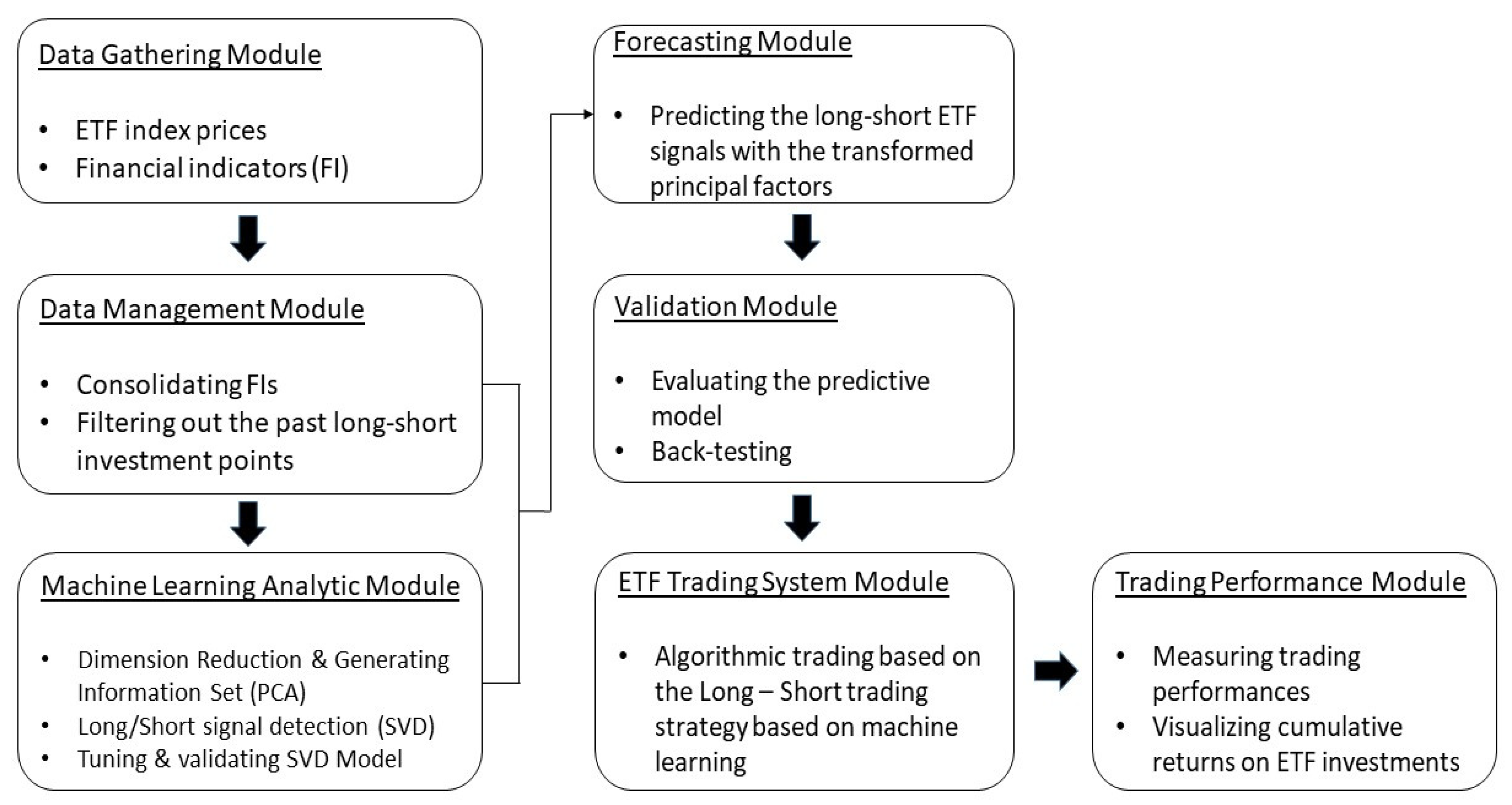
With the application of our model to ETF investments, we can develop the systemic structure of an algorithmic trading or a robo-advisor. Figure 1 summarizes the architecture of our trading system. To design this algorithmic system, we developed seven modules including data gathering, data management, machine learning analysis, forecasting long and short momentum patterns, model validation, ETF trading, and performance evaluations.

In order to develop our forecasting model, we split the dataset into a training sample and test sample. Our sample period was from December 2001 to December 2019. To build up the predictive model, we used 60% of the dataset (i.e., December 2001 to November 2011) as the training dataset. The remaining 40% of the dataset (i.e., December 2011 to December 2019) was for the hold-out test sample, which we used for cross-validation and robustness check. We evaluated the difference between predictive outcomes and realized results using the hold-out sample.

3. Empirical Results

3.1. Sample Data

We employed various datasets to develop our predictive model of ETF index trading. First, in order to develop the parsimonious principal factor, we gathered financial market indicators via the Bloomberg terminal and Federal Reserve Bank (FED) websites such as Chicago FED, Kansas City FED, and St. Louis FED.

We considered the following 16 market indicators as a set of proxies for market fundamentals associated with stock market movements. As shown in

Table 1. Financial risk indicators.

Index Type	Indicators
Financial Conditions Index	Conference Board Lending Credit Index
	Goldman Sachs Financial Condition Index
	Bloomberg Financial Condition Index
	Chicago FED National Activity Index
	Chicago FED National Financial Condition Index
	Kansas City FED U.S. Financial Stress Index
Money and Capital Market Index	TED Spread
	LIBOR and OIS Spread
	3-Month Commercial Paper and T-Bill Spread
	10-YR BAA Corporate Bond and T-Bond Spread
	Bloomberg-Barclays US Corporate High Yield OAS
	10-YR AA MUNI and T-Bond Spread
Volatility Index	Cboe Volatility Index
	Cboe S&P100 Volatility Index
	Cboe NASDAQ Volatility Index
	Cboe DJIA Volatility Index

, we selected three types of indicators: financial conditions indicators, money and capital market indicators, and market volatility indicators.

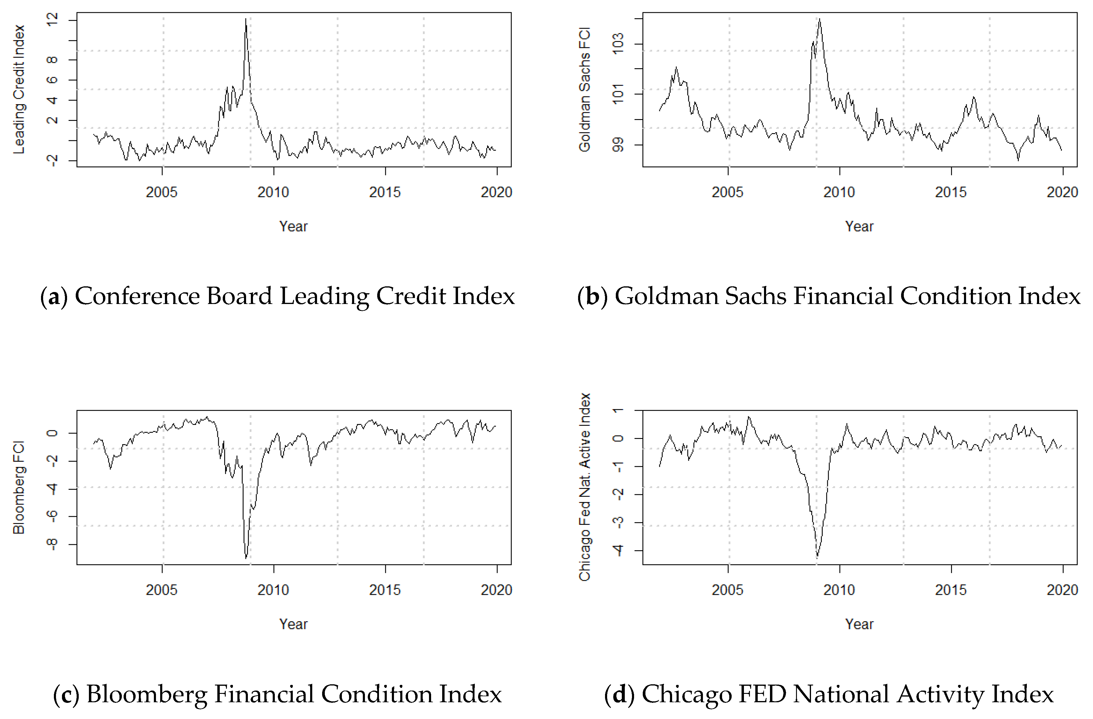
Following Levanon et al. [29] and Andreou et al. [30], we chose six indices to measure the financial conditions: Conference board leading credit index, Goldman Sachs financial conditions index, Bloomberg financial conditions index, Chicago FED national activity index, Chicago FED national financial conditions index, and Kansas City FED U.S. financial stress index. We collected the first three indicators using Bloomberg terminal and the remaining indicators from Federal Reserve Bank of Chicago and Kansas City.

Figure 2 displays these six financial conditions indicators over the period from December 2001 to December 2019. All six indicators show large variations during the sample period. Notably, they substantially fluctuated as the markets were exposed to systemic market events such as the dot-com crash (2001), 9/11 attack (2001), Lehman brothers bankruptcy (2008), flash crash (2010), European sovereign debt crisis (2010), and Chinese stock markets crash (2016) over the sample period. We observe a positive correlation between financial risk conditions and the Conference Board leading credit indictors, Goldman Sachs financial conditions index, and Kansas City FED U.S. financial stress index. By contrast, there is a negative correlation between financial risk conditions and the Bloomberg financial condition index, Chicago FED national activity index, and Chicago FED national financial condition index.

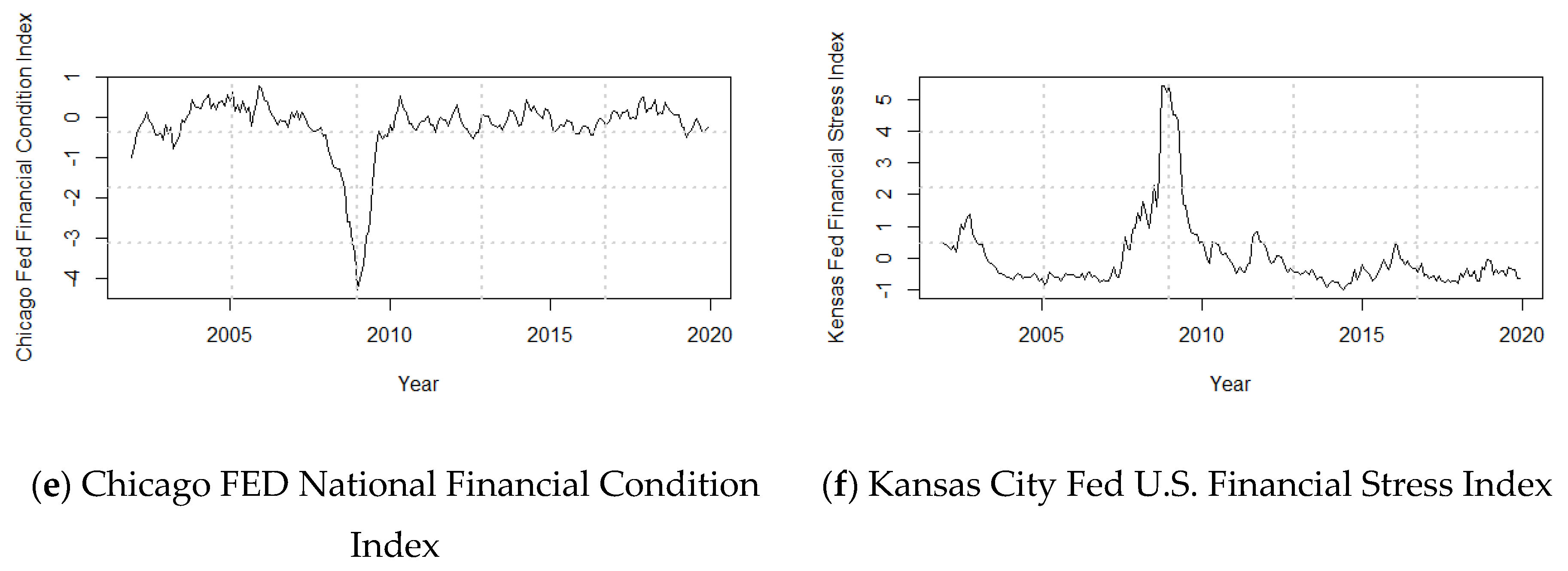
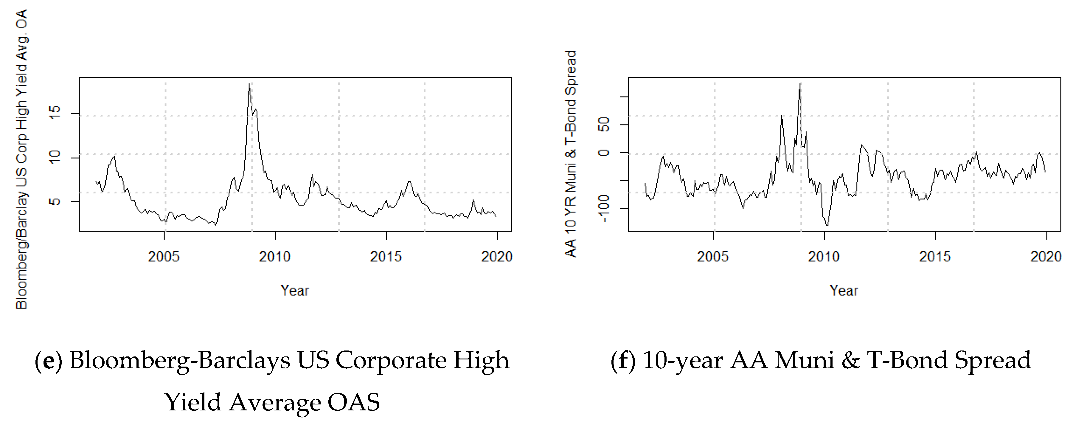
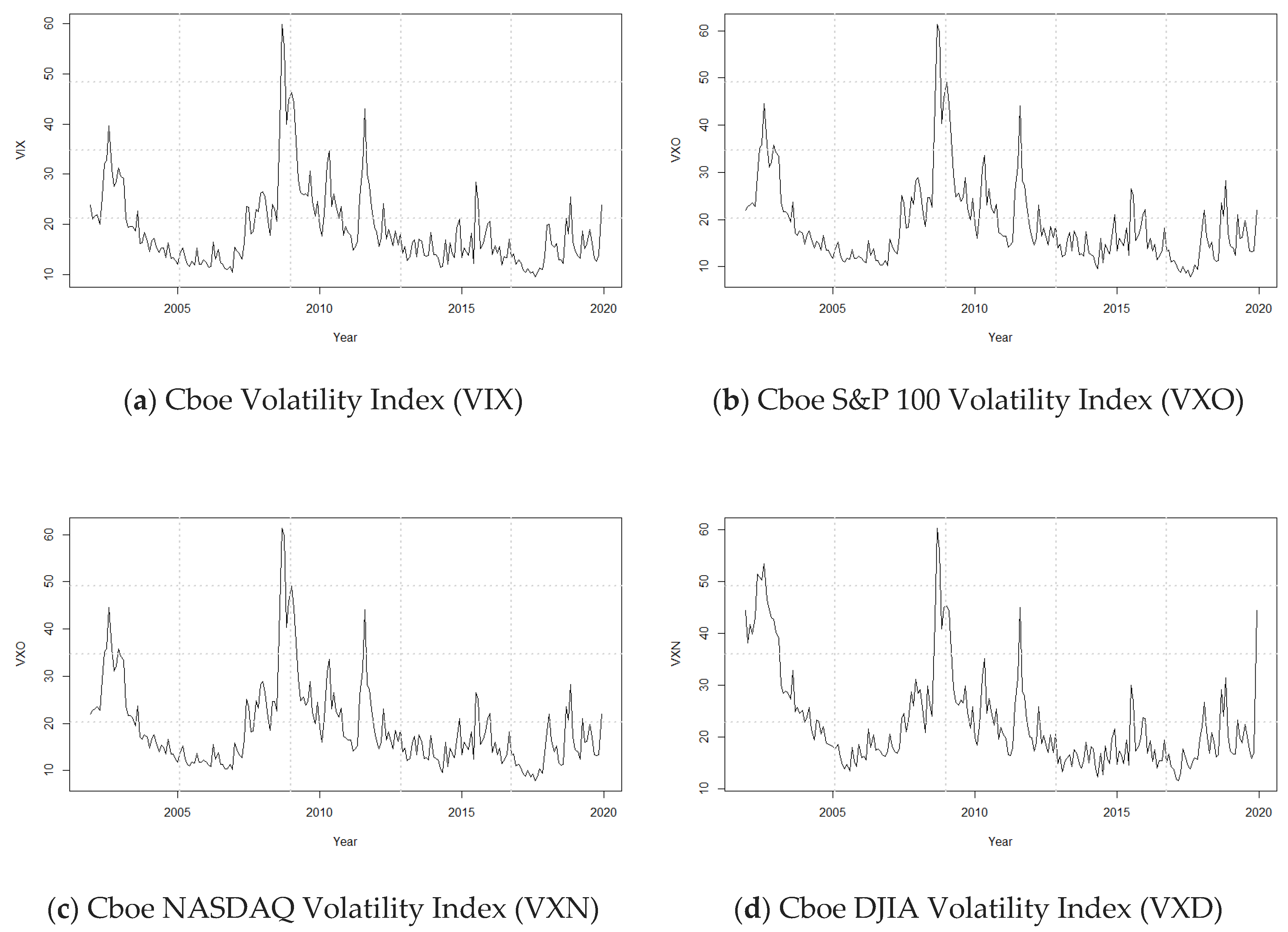
We also selected an additional six indicators for money and capital markets: TED spread, LIBOR and OIS spread, 3-month commercial paper and T-bill spread, 10-year BAA corporate bond and T-bond spread, Bloomberg-Barclays U.S. corporate high yield OAS, and 10-year AA municipal bond and T-bond spread. We collected the following fear indicators from Chicago Board Options Exchange (Cboe): Cboe volatility index, Cboe S&P100 volatility index, and Cboe NASDAQ volatility index. As shown in Figure 3 and Figure 4, the money and capital market indicators and the fear indicators responded to systemic market events.

Finally, in order to examine whether our predictive model can capture ETFs breakout patterns in the U.S., we selected the four largest ETF funds in the U.S. market: SPRD S&P 500 ETF trust (SPY), iShares Core S&P 500 ETF (IVV), Vanguard Total Stock Market ETF (VTI), and Invesco QQQ Trust Series 1 (QQQ). We used monthly data for the ETF funds from December 2001 to December 2019.

3.2. Extracting Parsimonious Factors with Principal Component Analysis

Table 2. Factor components and loadings.

Economic Risk Indicators	Factor 1 (Systemic Risk)	Factor 2 (Credit Risk)	Factor 3 (Fear Factor)
Panel A. Factor Loadings
Conference Board Leading Credit Index	−0.25	−0.28	0.06
Goldman Sachs Financial Condition Index	−0.23	0.32	−0.01
Bloomberg Financial Condition Index	0.29	0.02	−0.01
TED Spread	−0.21	−0.43	0.04
U.S. LIBOR and OIS Spread	−0.24	−0.31	0.00
3-Month Commercial Paper and T-Bill Spread	−0.22	−0.40	0.00
10-YR BAA Corporate Bond and T-Bond Spread	−0.28	0.02	−0.12
Bloomberg-Barclays US Corporate High Yield OAS	−0.27	0.17	−0.10
10-YR AA MUNI and T-Bond Spread	−0.18	−0.20	0.11
Chicago FED National Activity Index	0.25	0.02	0.41
Chicago FED National Financial Condition Index	0.25	0.02	0.41
Kansas City FED U.S. Financial Stress Index	−0.28	0.03	−0.14
Cboe Volatility Index (VIX)	−0.27	0.19	0.21
Cboe S&P100 Volatility Index (VXO)	−0.27	0.18	0.27
Cboe NASDAQ Volatility Index (VXN)	−0.23	0.24	0.45
Cboe DJIA Volatility Index (VXD)	−0.26	0.18	0.28
Panel B. Importance of Components
Proportion of Variance	69.5%	13.7%	5.5%
Cumulative Proportion	69.5%	83.2%	88.7%

summarizes our PCA results. Panel A shows factor loadings for each of the three factors. The first factor is in column 2. There are two groups of factor components in terms of the factor loadings. The first group is indexes with positive factor loadings, including Bloomberg financial conditions index, Chicago FED national activity index, Chicago FED national financial stress index. These three indexes show that the lower the index value, the worse are the market conditions. The second group is the components with the negative values including the remaining 13 indexes. Unlike the three indexes that are positively related to the economic conditions, these 13 indexes indicate that the market condition gets worse as their index value is higher. Since the absolute values of all the factor loadings stay around 0.25, we name the first factor as a systemic risk factor. Next, the second factor is reported in column 3. Notable factor loadings are TED spread (−0.43), U.S. LIBOR and OIS spread (−0.31), and 3-month commercial paper and T-bill spread (−0.40). These indices are associated with money and capital market risk. We define the second factor as a credit risk factor. Finally, the third factor is shown in column 4. Note that the factor loadings for Cboe Volatility Index, Cboe S&P100 Volatility Index, Cboe NASDAQ Volatility Index, Cboe DJIA Volatility Index, Chicago FED National Activity Index, and Chicago FED National Financial Condition Index are all greater than 0.20. Since these indexes measure the fear level of market participants, we view the third factor as a fear factor.

Panel B of Table 2 shows the explanatory power of each factor. Specifically, the first row reports proportion of variance that each of the three factors accounts for and the second row is the cumulative proportion. We find that our three factors cumulatively explain about 90% of total variation among them.

3.3. Momentum Patterns

In order to classify price momentum patterns (i.e., breakout signals), we first chose a size of movement in percentage terms. We arbitrarily selected 3% not to capture too many breakout price patterns. Next we split the price series into parts that have a percentage movement of at least 3% from beginning to end, but intervening movements of size of 3%. Lastly, we assigned a “+1” to each period of a part that consists of a move up, and assigned a “−1” to each period of the other part that consists of a move down. Following the above steps, we classified the price momentum patterns into two segments, a move up and move down, using monthly S&P 500 Index prices over the sample period. Based on the upward and downward momentums, we made segments of long and short intervals. Figure 5 displays the monthly S&P 500 Index prices and breakout patterns, setting a size of movement in percentage terms as 3%.

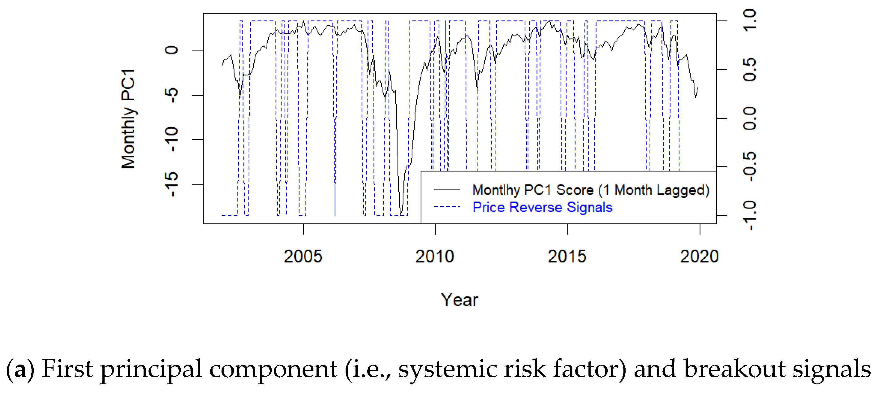
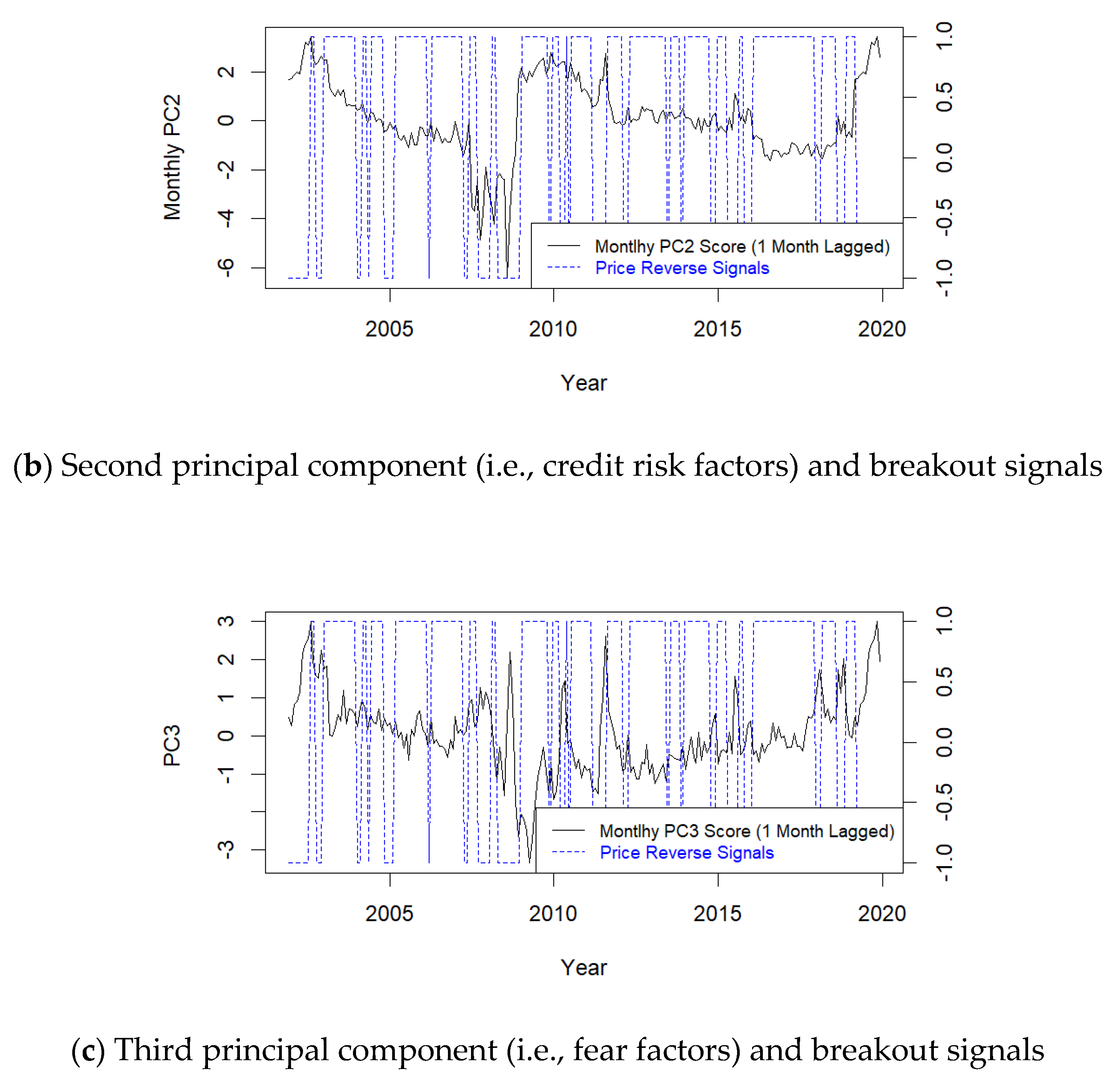
We then examined whether our three principal factors (systemic risk factor, credit risk factor, and fear factor) are significantly linked with momentum patterns. Figure 6 exhibits the relationship between the three principal factors and breakout signals captured from monthly S&P 500 Index prices over the sample period. Notably, all three principal factors and the breakout signals move closely together. The first principal factor (systemic risk) in panel (a) tends to move up in periods where the breakout signal is equal to +1, and to move down in periods where the signal is equal to −1. The second factor (credit risk) decreases when the breakout signal is in a short interval, and increases when the signal is in a long interval as shown in panel (b). This means that a downward momentum in equity assets appears when the credit risk in the U.S. stock market is high. The third factor (fear factor) in panel (c) shows a similar pattern to the second factor because the former is associated with market volatility: the fear factor displays a tendency to sharply increase when the breakout signal is −1, and to decrease when the signal is +1.

3.4. Developing Trading System Using SVM

We developed an algorithmic trading system using a predictive model based on our three factors (i.e., systemic risk factor, credit risk factor, fear factor) as well as past ETF price information. We set up a moving window of the past 24 months and computed exponentially the weighted moving averages. To forecast a long or short momentum trend one period ahead (i.e., $t+1$), we used contemporaneous risk factors and the exponential moving average at time $t$. We made our trading system determine a long or short investment decision based on SVM. Thus, we have our algorithmic trading system that (i) buys an ETF asset as our SVM model detects a turning point from downward price momentum to upward price momentum and (ii) sells an ETF asset when the forecasting model detects a turning point from upward price momentum to downward price momentum over the trading period.

Table 3. Algorithmic trading results over in-sample (training dataset).

ETF Funds	% of Wins	% of Fails	Drawdown	Return	Sigma	Comp. Return	Ann. SR
SPY	90.9	9.1	−0.01	0.18	0.20	1.78	8.94
IVV	92.3	7.7	−0.01	0.16	0.18	1.93	7.96
VTI	51.4	48.6	−0.26	0.02	0.10	0.54	0.61
QQQ	70.0	30.0	−0.12	0.10	0.15	1.96	3.89

presents the results of the machine learning trading for the four ETF assets (i.e., SPY, IVV, VTI, QQQ) over 109 months from November 2002 to November 2011. Over the in-sample trading period, our results indicate that the machine learning trading system which we developed performs well. In the second column, the percentage of total winning months over the trading months is greater than 70% except VTI. The monthly average returns over trading periods for each asset are positive. The average returns for SPY, IVV, VTI, and QQQ are more than 2% and all their compounding returns are more than 50%. All the annualized Sharpe ratios (SR) are positive (8.94 for SPY; 7.96 for IVV; 0.61 for VTI; 3.89 for QQQ). In particular, the Sharpe ratios for SPY and IVV are greater than 1.0, suggesting that our trading system shows a considerable performance in SPY and IVV assets. The drawdowns for SPY and IVV, which measure the worst peak-to-trough loss for the trading months, are substantially lower than those of other assets (1% loss for SPY and IVV; 26% loss for VTI; 12% loss for QQQ).

However, it is likely that the trading results in Table 3 are spurious because the trading model is developed based on the training dataset. In order to validate our trading system, we employed the out-of-sample data from December 2011 to December 2019.

Table 4. Algorithmic trading results over the hold-out sample (test dataset).

ETF Funds	% of Wins	% of Fails	Drawdown	Return	Sigma	Comp. Return	Ann. SR
SPY	66.7	33.3	−0.01	0.26	0.44	0.79	10.36
IVV	66.7	33.3	−0.01	0.27	0.44	0.80	10.40
VTI	75.0	25.0	−0.01	0.20	0.38	0.80	6.01
QQQ	57.1	42.9	−0.43	0.05	0.22	0.80	1.04

summarizes the trading performances during the 97 months. The percentage of total winning months is greater than 57%. Except for QQQ, the average monthly return for SPY, IVV, and VTI are greater than 20%. The standard deviations of the return range between 22% and 44%. The annualized Sharpe ratios are greater than 2.00 (10.36 for SPY; 10.40 for IVV; 6.01 for VTI; 1.04 for QQQ), which can be viewed as an extremely good trading strategy. The average of the annual Sharpe ratios is about 7.0, indicating that the additional amount of return that an investor receives from the ETF investment is, on average, seven times larger than its risk. Although the Sharpe Ratio of QQQ is 1.0 and its compounding return is 80% over the trading period, the drawdown of QQQ is relatively higher than that of other ETF assets. We conclude that the QQQ hurts the trading performance over the out-of-sample period.

In sum, we find that our machine learning system trading performances are robust to the sample periods. Most notably, our machine learning algorithmic trading system outperforms in SPY and IVV investments over the hold-out trading sample. Therefore, we view our trading model as a highly scalable machine learning trading strategy, especially in trading SPY and IVV.

4. Conclusions

AI and machine learning technology provide significant opportunities to invest in ETF index funds. This has been motivating research in AI and machine learning ETF trading models. The ETF index funds track underlying stock market indices such as S&P 500 Index, Dow Jones Index, and Nasdaq Index, meaning that the changes of the U.S. stock market indexes are associated with the U.S. ETF funds. Following the literature that shows the relation between the U.S. stock market indexes and financial indicators, unlike earlier machine learning ETF models that rely on the past ETF prices, we controlled for various financial indicators along with the past prices to build a predictive SVM factor model. Our predictive SVM factor model consists of three parsimonious risk factors (systemic risk factor, credit risk factor, and market fear factor), which are extracted from 16 financial risk indicators by PCA. Our results show that the factor model can detect the momentum patterns of ETF asset prices.

We further developed an algorithm trading system using our SVM factor model. To validate our trading model, we examined the trading performances for SPY, IVV, VTI, and QQQ over the in-sample and out-of-sample trading horizon. We found that the ETF trading system based on the SVM factor model has a good predictive power in detecting long/short signals over the in-sample and out-of-sample periods. We thus conclude that our proposed trading system is reliable and robust in trading the ETF assets. Finally, we find that our proposed trading system is promising in that the average of the annual Sharpe ratios obtained from the trading model using the out-of-sample data indicates the return that an investment would receive is seven times higher than the risk of holding the ETF index funds.

However, a caveat of our study is that our trading system in this paper is developed based on the U.S. ETF markets. In other words, our approach is limited to the U.S. ETF funds and the approach does not necessarily apply to other EFT markets. Based on our study, future research could make further contribution to the literature by developing a new system encompassing various ETF funds in the global markets.

References

- Artificial Intelligence and Machine Learning Are the Next Frontiers for ETFs, Says Industry Pro. Available online: https://www.cnbc.com/2019/08/24/artificial-intelligence-and-machine-learning-are-the-next-frontiers-for-etfs.html (accessed on 27 July 2020).
- Phoon, K.; Koh, F. Robo-Advisors and Wealth Management. J. Altern. Investig. 2018, 20, 79–94. [Google Scholar] [CrossRef]
- Poterba, J.M.; Shoven, J.B. Exchange-Traded Funds: A New Investment Option for Taxable Investors. Am. Econ. Rev. 2002, 92, 422–427. [Google Scholar] [CrossRef] [Green Version]
- Gastineau, G.L. Exchange Traded Funds. In Handbook of Finance; John Wiley & Sons, Inc.: Hoboken, NJ, USA, 2008; Volume 1. [Google Scholar] [CrossRef]
- Deville, L. Exchange Traded Funds: History, Trading, and Research. In Handbook of Financial Engineering; Springer: Boston, MA, USA, 2008; Volume 1, pp. 67–98. [Google Scholar] [CrossRef] [Green Version]
- Liew, J.K.; Mayster, B. Forecasting ETFs with Machine Learning Algorithms. J. Altern. Investig. 2018, 20, 58–78. [Google Scholar] [CrossRef]
- Li, M.; Zhao, X. Impact of Leveraged ETF Trading on the Market Quality of Component Stocks. N. Am. J. Econ. Financ. 2014, 28, 90–108. [Google Scholar] [CrossRef]
- Tse, Y.; Martinez, V. Price Discovery and Informational Efficiency of International Ishares Funds. Glob. Financ. J. 2007, 18, 1–15. [Google Scholar] [CrossRef]
- Tse, Y. Momentum Strategies with Stock Index Exchange-Traded Funds. N. Am. J. Econ. Financ. 2015, 33, 134–148. [Google Scholar] [CrossRef]
- Day, M.; Lin, J. Artificial Intelligence for ETF market prediction and portfolio optimization. In Proceedings of the 2019 IEEE/ACM International Conference on Advances in Social Networks Analysis and Mining, Vancouver, BC, Canada, 27–30 August 2019; pp. 1026–1033. [Google Scholar] [CrossRef]
- Lee, J. New Revolution in Fund Management: ETF/Index Design by Machines. Glob. Econ. Rev. 2019, 48, 261–272. [Google Scholar] [CrossRef]
- Li, Z.; Tam, V. A Machine Learning View on Momentum and Reversal Trading. Algorithms 2018, 11, 170. [Google Scholar] [CrossRef] [Green Version]
- Dimitriadou, A.; Gogas, P.; Papadimitriou, T.; Plakandaras, V. Oil Market Efficiency under a Machine Learning Perspective. Forecasting 2019, 1, 157–168. [Google Scholar] [CrossRef] [Green Version]
- Gupta, D.; Pratama, M.; Ma, Z.; Li, J.; Prasad, M. Financial Time Series Forecasting Using Twin Support Vector Regression. PLoS ONE 2019, 14, e0211402. [Google Scholar] [CrossRef]
- Kwon, C.S.; Shin, T.S. Cointegration and Causality between Macroeconomic Variables and Stock Market Returns. Glob. Financ. J. 1999, 10, 71–81. [Google Scholar] [CrossRef]
- Hong, H.; Torous, W.; Valkanov, R. Do Industries Lead Stock Markets? J. Financ. Econ. 2007, 83, 367–396. [Google Scholar] [CrossRef]
- Lettau, M.; Ludvigson, S. Consumption, Aggregate Wealth and Expected Stock Returns. J. Financ. 2001, 56, 815–849. [Google Scholar] [CrossRef] [Green Version]
- Black, A.J.; Klinkowska, O.; McMillan, D.G.; McMillan, F.J. Predicting Stock Returns: Do Commodity Prices Help? J. Forecast. 2014, 33, 627–639. [Google Scholar] [CrossRef]
- Hjalmarsson, E. Predicting Global Stock Returns. J. Financ. Quant. Anal. 2010, 45, 49–80. [Google Scholar] [CrossRef] [Green Version]
- Bernanke, B.; Kuttner, K. What Explains the Stock Market’s Reaction to Federal Reserve Policy? J. Financ. 2005, 60, 1221–1257. [Google Scholar] [CrossRef] [Green Version]
- Campbell, J.; Vuolteenaho, T. Inflation Illusion and Stock Prices. Am. Econ. Rev. 2004, 94, 19–23. [Google Scholar] [CrossRef] [Green Version]
- Cooper, I.; Priestley, R. Time-Varying Risk Premiums and the Output Gap. Rev. Financ. Stud. 2008, 22, 2801–2833. [Google Scholar] [CrossRef]
- Maio, P. The “Fed Model” and the Predictability of Stock Returns. Rev. Financ. 2013, 17, 1489–1533. [Google Scholar] [CrossRef]
- Billio, M.; Getmansky, M.; Lo, A.W.; Pelizzon, L. Econometric Measures of Connectedness and Systemic Risk in the Finance and Insurance Sectors. J. Financ. Econ. 2012, 104, 535–559. [Google Scholar] [CrossRef]
- Baek, S.; Cursio, J.D.; Cha, S.Y. Nonparametric Factor Analytic Risk Measurement in Common Stocks in Financial Firms: Evidence from Korean Firms. Asia-Pac. J. Financ. St. 2015, 44, 497–536. [Google Scholar] [CrossRef]
- Vapnik, V. The Nature of Statistical Learning Theory; Springer Science & Business Media: Berlin/Heidelberg, Germany, 1995. [Google Scholar]
- Alexeev, V.; Tapon, F. Testing Weak Form Efficiency on the Toronto Stock Exchange. J. Empir. Financ. 2011, 18, 661–691. [Google Scholar] [CrossRef]
- Park, C.; Irwin, S. What Do We Know about the Profitability of Technical Analysis? J. Econ. Surv. 2007, 21, 786–826. [Google Scholar] [CrossRef]
- Levanon, G.; Manini, J.; Ozyildirim, A.; Schaitkin, B.; Tanchua, J. Using Financial Indicators to Predict Turning Points in the Business Cycle: The Case of the Leading Economic Index For the United States. Int. J. Forecast. 2015, 31, 426–445. [Google Scholar] [CrossRef]
- Andreou, E.; Ghysels, E.; Kourtellos, A. Should Macroeconomic Forecasters Use Daily Financial Data and How? J. Bus. Econ. Stat. 2013, 31, 240–251. [Google Scholar] [CrossRef]
Figure 1.
Architecture of the machine learning trading system for exchange traded fund (ETF) index funds.
Figure 2.
Financial Conditions Indicators: (a) Conference Board Leading Credit Index, (b) Goldman Sachs Financial Condition Index, (c) Bloomberg Financial Condition Index, (d) Chicago FED National Activity Index, (e) Chicago FED National Financial Condition Index, (f) Kansas City Fed U.S. Financial Stress Index.
Figure 3.
Money and Capital Market Indicators: (a) TED Spread, (b) LIBOR & OIS Spread, (c) 3-month Commercial Paper & T-bill Spread, (d) 10-year BAA Corp. Bond & T-Bond Spread, (e) Bloomberg-Barclays US Corporate High Yield Average OAS, (f) 10-year AA Muni & T-Bond Spread.
Figure 4.
Chicago Board of Options Exchange Volatility Indexes: (a) Cboe Volatility Index (VIX), (b) Cboe S&P 100 Volatility Index (VXO), (c) Cboe NASDAQ Volatility Index (VXN), (d) Cboe DJIA Volatility Index (VXD).
Figure 5.
Monthly S&P 500 Index prices and breakout patterns.
Figure 6.
Monthly principal factors and breakout signals from S&P 500 Index: (a) First principal component (i.e., systemic risk factor) and breakout signals, (b) Second principal component (i.e., credit risk factors) and breakout signals, (c) Third principal component (i.e., fear factors) and breakout signals.