Article

A Complementary Approach to Traditional Energy Balances for Assessing Energy Efficiency Measures in Final Uses: The Case of Space Heating and Cooling in Argentina

1
Department of Mathematics, Faculty of Exact Sciences, Engineering and Surveying, National University of Rosario, Rosario 2000, Argentina
2
Department of Energy, Polytechnic University of Milan, 20156 Milan, Italy
*
Author to whom correspondence should be addressed.
Sustainability 2020, 12(16), 6563; https://0-doi-org.brum.beds.ac.uk/10.3390/su12166563
Submission received: 18 July 2020 / Revised: 8 August 2020 / Accepted: 11 August 2020 / Published: 13 August 2020
(This article belongs to the Special Issue Energy Efficiency and Comfort Indoor in Smart Buildings)

Abstract

:
Energy balances have been historically conceived based on a supply-side perspective, providing neither detailed information about energy conversion into useful services nor the effects that may be induced by the application of policies in other sectors to energy consumption. This article proposes an approach to a thorough assessment of the impact of efficiency policies on final energy uses, focusing on residential space heating and cooling, and capable of: (1) quantifying final useful services provided and (2) accounting for the global impact of efficiency policies on final energy use, taking advantage of Input–Output analysis. This approach is applied in five cities of Argentina. Firstly, the quantity of energy service provided (i.e., level of thermal comfort) for each city is evaluated and compared with the defined target. It is found out that heating comfort is guaranteed approximately as established, whereas in the cooling case the provision is twice the established level. Secondly, primary energy consumption of heating and cooling services is evaluated before and after different efficiency improvement policies. The results show that the major primary energy saving (52%) is obtained from the upgrading appliances scenario and reflect the importance of accounting for embodied energy in goods and services involved in interventions.

1. Introduction

In recent years, great efforts have been made by different countries to increase the efficiency of energy systems in order to reduce emission wastes, local pollutants and greenhouse gases. In the global efficiency of energy systems, final consumption plays an essential role which, according to the International Energy Agency, may actually set the basis for making several improvements in terms of energy efficiency [1]. The implementation of policies on energy efficiency regarding final consumption provides governments with a challenge since, unlike supply, consumption sectors have been historically left aside, particularly in developing countries. Traditional approaches to energy system analysis are still largely supply orientated, i.e., focusing on the management of energy conversion, production and distribution, and the final use of energy in the form of energy carriers [2]. The main challenge consists in giving an integral overview of both primary resources and the end of the energy flow [3], thinking of overall energy system efficiency as the benefits or services that systems provide in relation to the primary energy resources involved [4]. Under this approach, final consumption is as important as all the other stages (production, transformation, transport, distribution) in terms of public energy efficiency policies [5]. So, in order to improve final consumption efficiency, it is first necessary to have detailed information about it, and to integrate that information to the entire energy system analysis [6].
Energy balances are the backbone of energy system analysis, and because of the history of their development, the currently adopted balance methodologies are made from the supply perspective, without detailed treatment of consumption data [7], as this aspect was originally felt to be outside their scope. In particular, they do not quantify benefits obtained from energy use (i.e., energy services) [8,9] and they do not reflect the relationship between consumption sectors (i.e., embodied energy in goods and services). Hence, they have great limitations regarding the information provided about final use, constituting an important barrier to the implementation of end-use energy efficiency policies.
Therefore, it is necessary to develop information systems for complementing current energy balance methodologies, providing detailed information about final consumption that is capable of quantifying energy services, and reflecting the interaction between different consumption sectors in order to assess the real primary resources involved in the provision of certain amounts of energy service. In addition, these methodologies must be easily applicable, relying on simple and available data as inputs, and providing comparable results when applied in different countries or regions.
The objective of this research is to propose an approach to complement traditional energy balances by including final energy service stages (here focusing on space heating and cooling services), and to assess the economic and environmental impacts of efficiency policies and interventions at a nationwide scale. Firstly, the provision unit is presented to quantify the energy services (i.e., a measure of the quantity of energy service provided), and for its definition, technological aspects and climatic and socioeconomic conditions are considered (in the same way that certain conditions must be specified when defining a physical unit of measurement). Secondly, Input–Output analysis is suggested as a suitable approach to assess the overall impact due to energy efficiency improvements in final consumption (e.g., energy policy interventions, technology shifts, etc.), considering the direct and indirect economy-wide effects caused by the proposed improvement [10].
The methodology is then applied to a case study in Argentina, defining heating and cooling provision units of five of its major cities so as to truly reflect different climatic and socio-economic situations: Rosario, Mendoza, San Carlos de Bariloche, San Miguel de Tucumán and Buenos Aires; determining their coverage level (i.e., the quantity of energy service actually guaranteed in each city); and finally assessing the change in nationwide primary energy consumption due to final use efficiency improvement scenarios.
In Argentina, the correlation between energy consumption and GDP is still high, which shows the country’s small incursion into energy efficiency [11]. Furthermore, the primary energy supply matrix is approximately 86% fossil fuel, so energy efficiency policies could lead to a significant reduction in greenhouse gas emissions [12]. Since 2002, subsidies have acted as the main barrier to end-use energy efficiency policies [13], there is poor regulation [14] and the lack of information prevents effective policies from being established [15]. Building codes do not require isolation standards (with some exceptions, such as in Rosario since 2012 and recently in Buenos Aires, Olavarría) [16]. The lack of regulations and subsidies has led to very high thermal requirements, and in cold areas, energy consumption for space heating is several times the consumption in European cities with a similar climate [17]. In 2018, the national building certification program was launched with the aim of establishing a certification process for the entire country. So far, pilot tests for building certification have been carried out in seven locations [18]. This research contributes to the attempts and advances in assessing the benefits of energy use, and the primary energy requirements associated with such uses. The main novelty of the proposed methodology is that it can quantify primary energy resources involved in the provision of a certain amount of energy service and assess overall impacts due to energy efficiency improvements in that provision as well. Moreover, the application of the methodology is rather simple as it only requires commonly available statistical data with no need for additional surveys or data collection.
The rest of the article is organized as follows: in Section 2, a literature review is presented; in Section 3, the novel methodology is formalized, while in Section 4 reference data and assumptions are established and final consumption scenarios are defined for the application in Argentina. The results are then presented in Section 5, and Section 6 summarizes the final conclusions and remarks.

2. Literature Review

In this section, a brief literature review is presented, related to four main areas: (a) energy efficiency indicators, (b) energy service quantification; (c) extensions of energy balance and (d) energy accounting based on Input–Output methods.
Energy efficiency describes the ratio between the benefits gained and the energy used. Irrek and Thomas distinguish different approaches concerning energy efficiency: macro-economic; energy conversion between supply and provision; end use on the demand side and energy efforts of the human body in household production of the caring economy [19]. Oikonomou et al. define efficiency as the ratio between energy input and output services that can be modified with technical improvements (e.g., technology substitution) and differentiate it from the concept of energy saving, linked to human behavior [20]. Patterson defines a series of indicators used to measure energy efficiency from a physical and economic perspective, focusing on the energy consumption caused by each segment of the national economy, concluding that more attention needs to be given by policy analysts to manage this concept [21]. Tanaka explores different ways to measure energy efficiency performance: absolute energy consumption, energy intensity and the diffusion of a specific energy-saving technology or thermal efficiency [22]. Haas defines energy efficiency indicators for the residential sector, considering key factors for their normalization and comparison, concluding the need for more disaggregated indicators and lifestyle studies [23]. In that sense, Pérez-Lombard et al. revise the main methodological problems for the construction of energy efficiency indicators and propose a sequence of actions to tackle these problems in an ordered fashion: establishing the service quality, identifying aggregation levels on the efficiency pyramid, defining a magnitude for consumption measurement and choosing a suitable magnitude to quantify the service provided [24].
The most widespread energy efficiency indicator is the energy intensity of a country, defined as the primary energy needed to generate a unit of gross domestic product [25]. Little can be said, on the basis of that ratio, about why energy use for any sector has reached a certain level, how efficient that use is, or why use varies so much between otherwise similar countries [26]. In that sense, Schipper et al. review a series of sectorial indicators and exemplify 14 countries based on six sectors of energy use. With the same approach, the International Energy Agency presents a decomposition analysis with the aim of identifying the causes of changes in energy demand, by separating the role of activity and structural changes to isolate changes in energy intensity due to energy efficiency [8]. The decomposition analysis of energy consumption is also considered in the Odyssee-Mure Project as a tool to contribute to the evaluation of national energy efficiency policies and analyze the keys to their successful implementation [27]. Elsewhere, the Eurostat methodology for statistics on energy consumption in households [7] refers to a list of relevant variables that shape consumption (e.g., demographic and social variables, dwelling variables, energy technologies).
Regarding the energy service concept, its definition is not unified in the academic field. Fell reviews different uses and meanings in the literature, highlighting the disparity of approaches to it [28]. The same conclusion is obtained by Kalt et al. after reviewing the energy service concept in different areas, and consequently propose the Energy Service Cascade Framework for establishing a more consistent understanding of how energy use contributes to human well-being [29]. Different energy service definitions can be grouped into three categories: (I) those which refer to useful energy (e.g., heat, available work, etc.), as proposed by Sorrell “We define energy service as the useful work obtained by energy consuming” [30]; (II) those which refer to some kind of benefit, exemplified in the definition “Energy services are the benefits that energy carriers produce for human well-being” [31]; and finally (III) those which refer to a result of energy conversion or a combination its use with technology and use as proposed by Fouquet “Energy services refer to the services that are generated from consuming energy combined with appliances” [32]. Several pieces of research involving different energy service meanings can be cited, for example: Sovacool (group I) identifies how energy services differ according to sectors and income, concluding that focusing on energy services reorients the direction of energy policy interventions [33]; Cravioto et al. (group II) explore the link through such a concept by analyzing how 17 predictors associate with six dimensions of energy service satisfaction in two income groups in Mexico [34]. Cullen et al. (group III) trace the global flow of energy, from fuels through to the final services, and focus on the technical conversion devices and passive systems in each energy chain. They introduce the term passive system as the last technical component in an energy chain [4]. This concept of tracing energy flow through to final services was first explored by Nakicenovic and co-authors in the early 1990s [35,36,37]. They introduce the term service efficiency, defined as the provision of a given task with less useful energy (the output from conversion devices) without loss of service. In the same way, Flórez-Orrego et al. present a comparative exergy and environmental analysis of vehicle fuel end use in Brazil, and consider that a car is a product used to deliver a transportation service, i.e., the physical movement of a material over a distance within a given time [38].
Regarding the extension of energy balances to the useful stage, previous works can be divided in two main groups: societal exergy analysis and extended exergy accounting. The societal exergy analysis emerged based on the works of Reistad, Wall and Kümmel [39,40,41]. Ayres et al. study physical flows in endogenous growth models, the role of physical work in economic growth [42,43] and the impact of resource consumption and technological change on economic growth [44]. Serrenho standardizes the allocation of final energy to useful exergy categories [45], while Brockway improves the accuracy of exergetic efficiency estimates [46]. The extended exergy accounting, conceived by Sciubba [47], consists in the evaluation of the total equivalent primary resource consumption in a generic system [48]. An extensive review of extended exergy accounting is carried out in [49].
The use of Input–Output analysis (IOA) for analyzing relations between the economy and environment has increased in recent years [50]. Currently, IOA is a widely adopted method for the classical study of different economies and environmental impact analysis [10]. In the energy field, IOA is a powerful tool to account for the energy directly and indirectly consumed by households (i.e., the energy embodied in goods and services) under a consumption-based approach (CBA) [51]. Chen et al. compare IOA with two other methods for urban energy use in Beijing, highlighting the different perspectives and results [52]. Other studies compare CBA based on IOA versus a production-based approach (PBA) for Chinese industries [53] and the South African economy [54]. Owen et al. contrast two different modes of energy resource allocation for the UK, showing that extracted energy and used energy allocation vectors produce similar estimations of the overall energy consumption accounting [55]. Besides, IOA is also used for understanding energy embodied in interregional consumption and trade, for example, China’s construction industry [56] and energy flow structure in China’s regions [57]. Rocco et al. formalize international trade treatment methods in IOA and apply it to a case study based on the World Input–Output Database [58]. Recently, Heun et al. proposed a physical supply–use table energy analysis framework from which the IO structure of an energy conversion chain can be determined and the effects of changes in final demand can be estimated [59].
To sum up, the review of the literature indicates the following fundamental aspects: the necessity of complementing traditional energy balances with information about final and useful energy consumption stages; the need to unify the energy service concept; the need to define methods to quantify energy services in order to measure the benefits obtained from energy use; the need to integrate such extended energy statistics with Input–Output methods and models to provide an economy-wide assessment of expected policy impacts.

3. Methods and Models

This section introduces and formalizes an approach to quantifying energy services and assessing the impact of expected policy shocks at a country-wide scale. The proposed approach is based on the extension of traditional energy balance to energy services, quantifying them by means of the provision unit concept, and on the link between the extended energy balance and a meso-economic Input–Output model. This approach enables us to assess the sectoral primary energy requirements before and after improvements in final use efficiency. The formalization is here presented for heating and cooling services as part of residential final consumptions, but it can, in principle, be extended and generalized to other energy services as well.

3.1. Provision Unit Definition and Evaluation

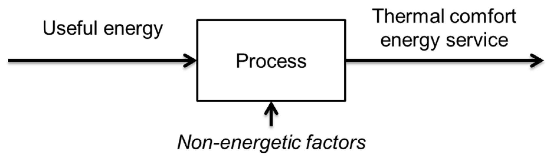
The generation of a heating or cooling provision unit can be conceptualized as a process (Figure 1), whose input is thermal energy (in any direction) and whose output is the thermal comfort state energy service. For obtaining that thermal comfort, the amount of thermal energy required will be conditioned by non-energetic factors such as the type of building, envelope characteristics, climate and other exogenous variables, i.e., passive systems [4].

3.1.1. Definition of Heating and Cooling Provision Units

The heating and cooling provision units P U h ; o b j ; P U c ; o b j ( k W h / p ) are defined as the necessary useful energy for guaranteeing the thermal comfort of a person (i.e., energy service), under pre-established climatic zone conditions c z h   ; c z c , comfort conditions c h ;   c c and the socio-economic condition s e during heating and cooling periods. Expression (1) shows the mathematical formalization.
P U h ; o b j = c z h c h s e P U c ; o b j = c z c c c s e
Comfort conditions c h ; c c account for the level of comfort provided. They consider the number of comfort days guaranteed D c o m f ; h ; D c o m f ; c (or the number of equivalent days if the comfort profile is defined in hours), the total number of heating or cooling days of the i-th month D i and the total number of months M h ; M c of the heating and cooling period correspond to the climatic zone condition (2). The determination of D c o m f ; h ; D c o m f ; c must be done considering short-term economic indicators (e.g., employment, inflation, energy prices, family spending, confidence) or quantifying cultural characteristics (e.g., by means of surveys).
c h = D c o m f ; h i = 1 M h D i ; c c = D c o m f ; c i = 1 M c D i
The socio-economic condition s e ( m 2 / p ) takes into account the level of structural well-being of a population and its housing standards. It takes into account average values of building floor area A ( m 2 ), the fraction of conditioned floor area a and building occupancy O ( p ) (3).
s e = A a O
While the comfort condition shows characteristics of rapid variation, the socio-economic condition reflects the structural and long-term standards of a population. Because of this, they must be considered separately [60]. Furthermore, the socio-economic condition assumes the same value for heating and cooling cases.
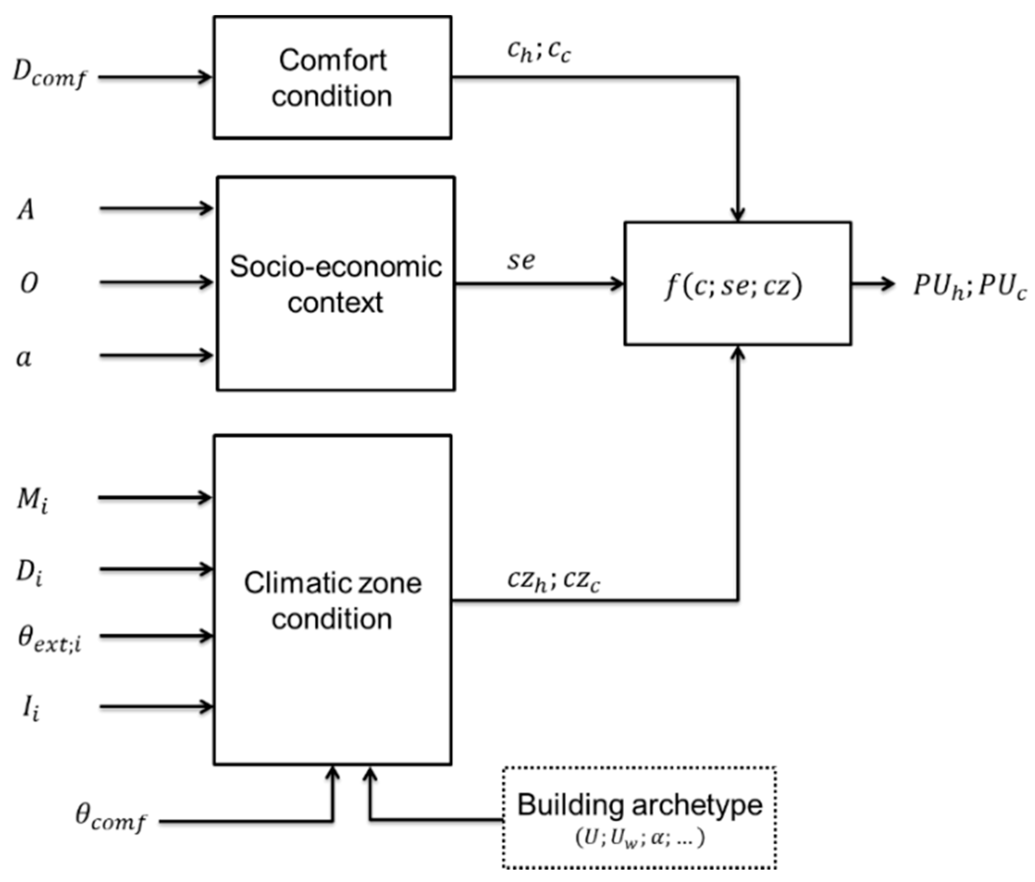
Climate zone conditions c z h ; c z c ( k W h / m 2 ) show the climatic zone characteristics. They are calculated as the thermal requirement of a building archetype for all the heating and cooling periods. A building archetype consists in an abstract entity that enables an energy requirement calculation in different locations, in order to capture distinct climatic zone characteristics. Because of this, the building archetype must be unique for all the cities of the country or region being analyzed, consequently leading to comparable results. There are several ways to establish the building archetype, and local advisors are in charge of doing so. It can be a real building, or defined by specific thermal properties on a per square meter basis instead, according to Table 1. For thermal energy requirement determination, both heating and cooling comfort temperatures θ c o m f ; h ; θ c o m f ; c (i.e., set-point temperatures) are also needed. There are several methods of thermal energy calculation, and the adoption of national energy performance labeling procedures is suggested for this purpose. A simplified method based on ISO 13790:2008 [61] is presented in Appendix A as a suitable alternative for those countries that have not developed such procedures yet.
Figure 2 schematizes the input variables for calculating c z , c and s e and the role of the building archetype in the determination of provision units.
Once the provision units for heating and cooling in different cities are established, it is useful to define a location as a reference location for comparison purposes. Thus, reference provision units P U h ; o b j ; 0 ; P U c ; o b j ; 0 are calculated for the reference city.
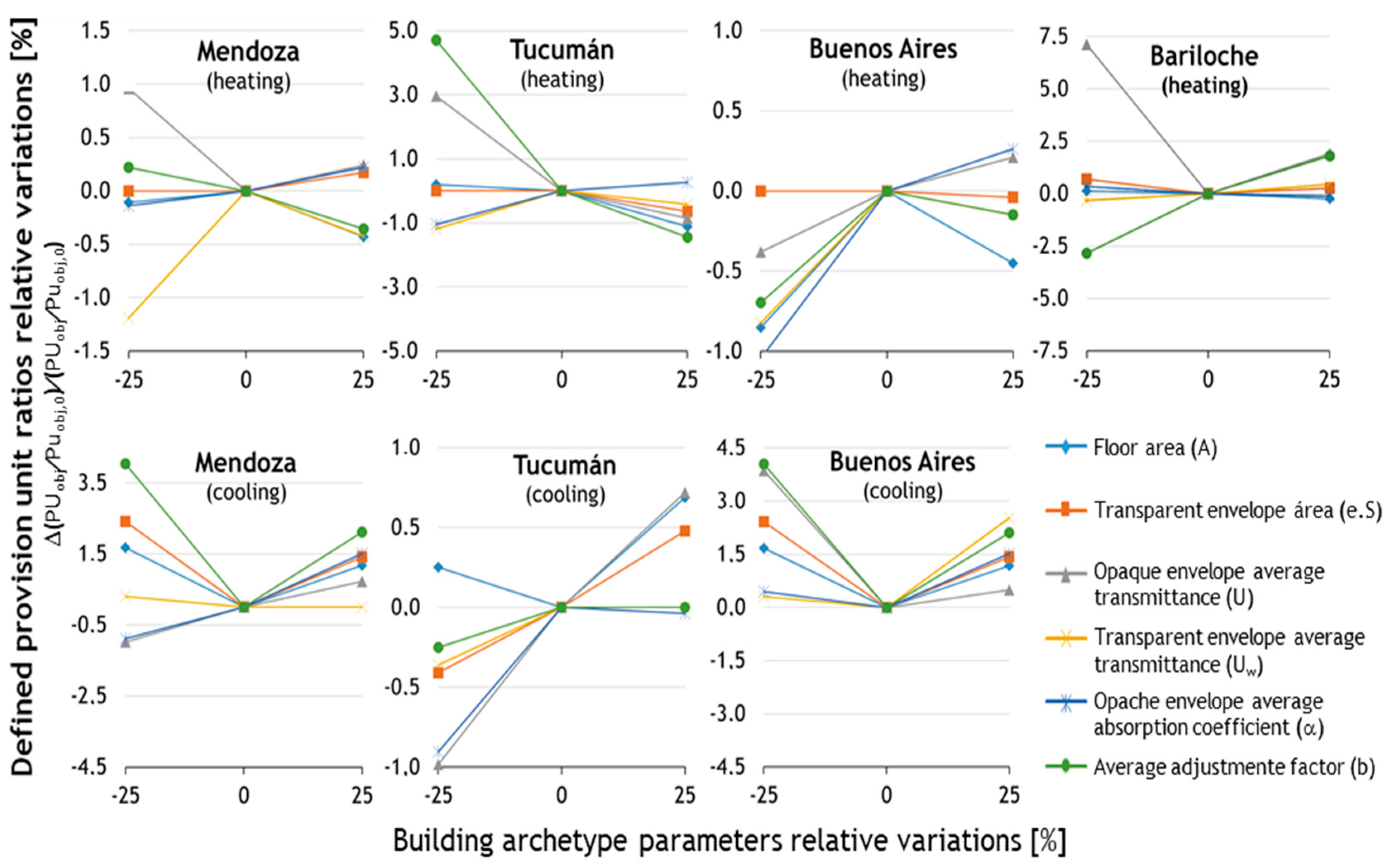
Although the building archetype determines the value of c z , its introduction is just a tool that makes calculation possible. The relationship between a climatic zone condition and the reference one c z / c z 0 should be insensitive to building archetype parameters, in order to affirm the method robustness. Considering ε as any parameter of the building archetype, and ρ as a superior limit that is as small as desired, Expression (4) should be verified for the most relevant building archetype parameters.
| ( c z c z 0 ) ε Δ ε ( c z c z 0 ) | < ρ

3.1.2. Provision Units, Energy Requirements and Consumptions

By defining provision units, a new unit of the measure of energy services is available. Thus, a deeper analysis of final consumption can be carried out in order to understand the drivers of secondary energy consumption and to compare the quantity of energy service guaranteed in different locations as well.
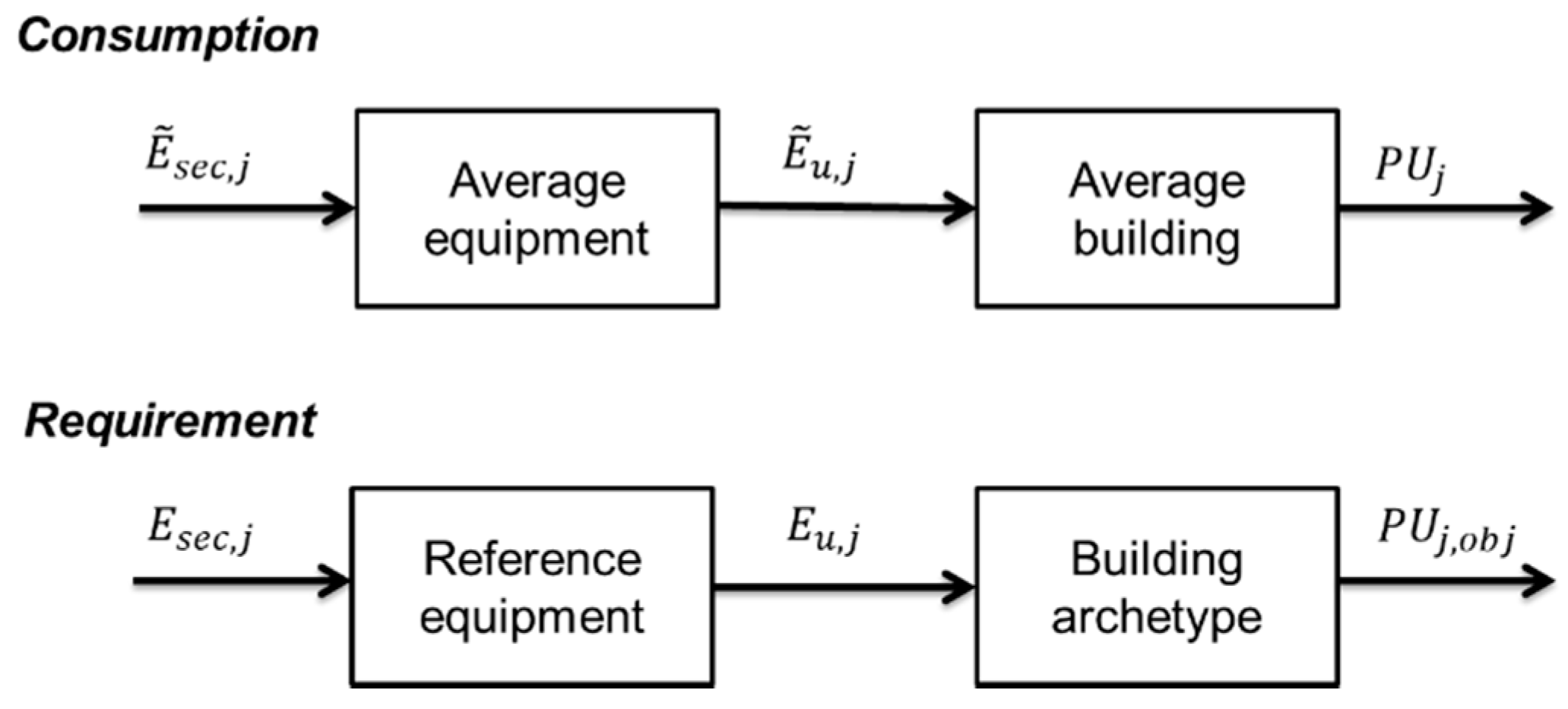
It is worth noting that consumptions and requirements both refer to energy, however, real consumption E ˜ (measurable) will not be necessarily equal to theoretical requirement E (estimated by calculation methods). The most immediate differences are produced by uncertainties in the theoretical model and in the parameters involved. In addition, there exist other causes of differences between consumption and requirement. Considering an ideal case in which energy requirement calculation predicts consumption exactly, there are three possible situations that could lead to dissimilarities between requirement and real consumption related to provision unit j. (see Figure 3):
  • Differences in the provision unit ( P U j P U j ; o b j ): equipment efficiencies are equal to the reference ones, the thermal characteristics of buildings are the same as those adopted for the building archetype, but the provision unit defined for the location is not totally guaranteed or is excessively guaranteed.
  • Differences in useful energy ( E ˜ u ; j E u ; j ): equipment efficiencies are equal to the reference ones, the thermal characteristics of buildings are different from those adopted for the building archetype, and the provision unit is guaranteed exactly as defined for the location.
  • Differences in secondary energy (carrier) ( E ˜ s e c ; j E s e c ; j ): equipment efficiencies are different from the reference ones, the thermal characteristics of buildings are equal to those adopted for the building archetype, and the provision unit is guaranteed exactly as defined for the location.

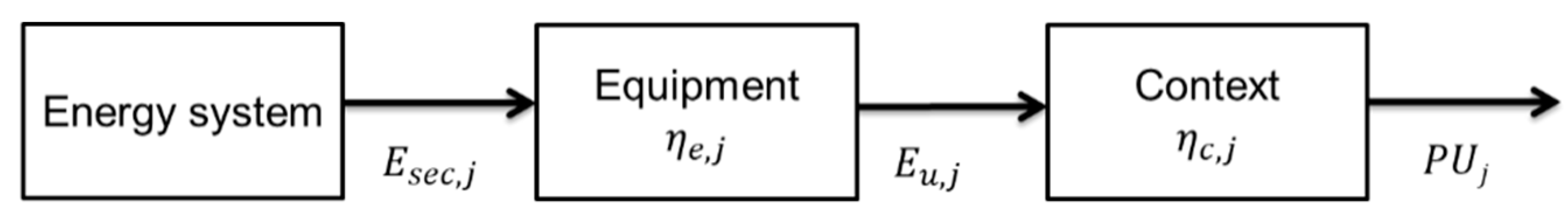
3.1.3. Energy Balance Extension for Heating and Cooling Uses

Provision units can be coupled with traditional energy balances. Figure 4 shows an energy flow diagram from the energy system to the provision unit j ( P U j ). Thus, for the extension proposed, equipment efficiency η e ; j and context efficiency η c ; j must be defined. The context efficiency relates the non-energetic provision unit (i.e., quantity of energy service) with the useful energy needed to produce it. Although it does not relate two energies, it is formally like an efficiency.
In order to determine context efficiency, a comparison between the population average building and building archetype must be made (for heating and cooling provision units separately). The ratio between the climatic zone factor calculated with the building archetype c z j ( b u i l d i n g _ a r c h e t y p e ) and the factor calculated with the average building c z j ( a v e r a g e _ b u i l d i n g ) is a suitable way (5); nevertheless, local advisors could also develop other mechanisms for characterizing buildings’ thermal properties and arrive at a dimensionless context efficiency value as well (Expression (5) could be larger than one, meaning that the building archetype would need more thermal energy with respect to the average building to guarantee the established comfort in a considered climatic zone). Equipment efficiency can be obtained from traditional useful energy balances or energy surveys.
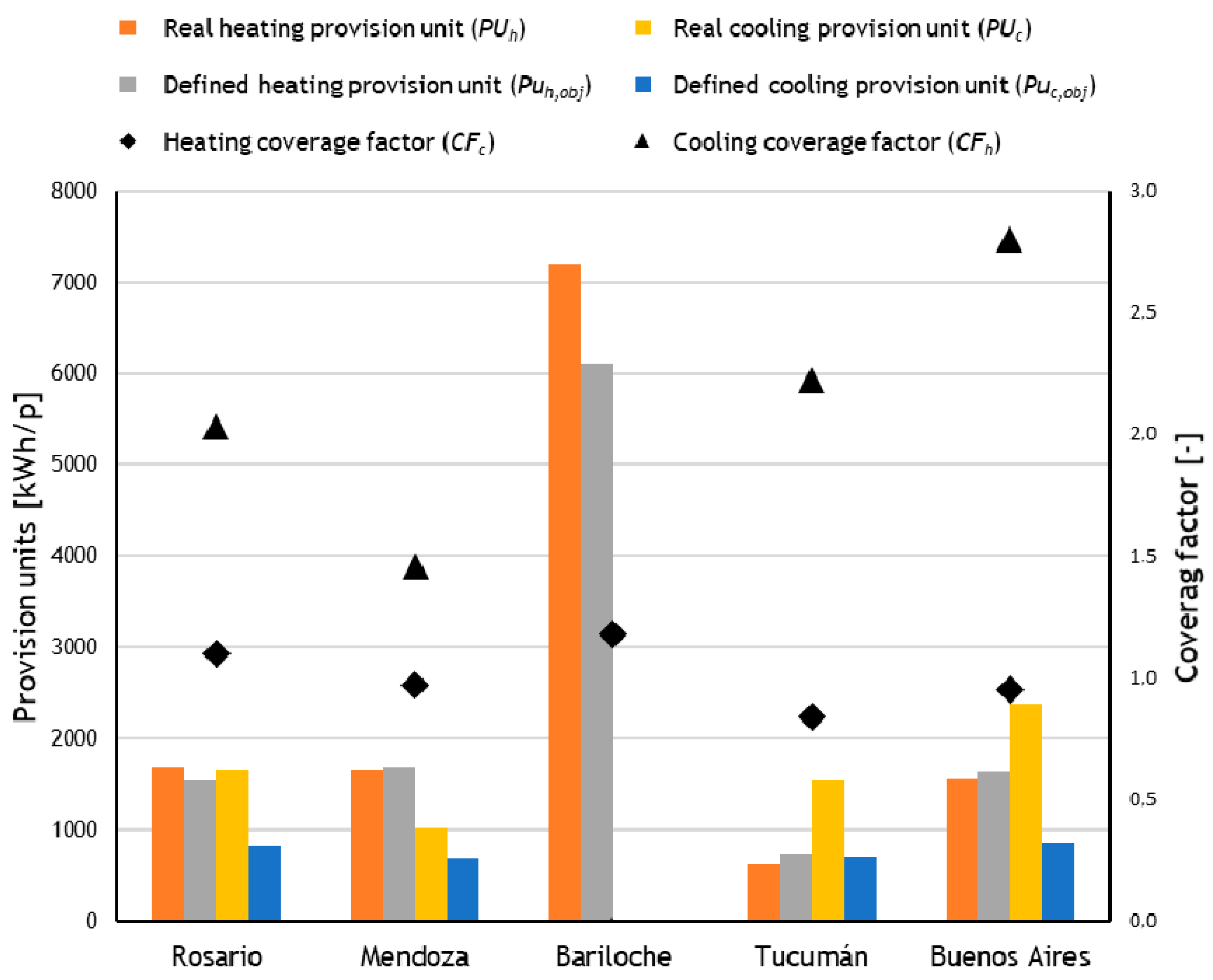
η c ; j = c z j ( b u i l d i n g _ a r c h e t y p e ) c z j ( a v e r a g e _ b u i l d i n g )
Once the provision unit j for the location P U j ; o b j has been established, and knowing secondary energy consumption associated with that use E ˜ s e c ; j , it is possible to calculate the real provision unit P U j and its coverage factor C F j according to Expressions (6) and (7). In the same way, once reference values for context and equipment efficiencies have been adopted, secondary energy requirement E s e c ; j can be obtained according to Expression (8).
P U j = E ˜ sec ; j η e ; j η c ; j
C F j = P U j P U j ; o b j
E sec ; j = P U j ; o b j η e ; j ; 0 η c ; j ; 0
Coverage factor gives evidence of the level of energy service guaranteed, and it can be used as a quantitative proxy for indicating the benefit gained from the energy system.
Expressions (6) and (7) assume a single energy carrier for the considered use. In case a provision unit is obtained from many carriers, new efficiencies and conversion factors should be calculated as weighted averages based on each carrier participation (e.g., a heating system operating with natural gas and electricity).

3.2. Assessing the Effects of Policy Interventions Based on Input–Output Analysis

Expressions (6) and (7), as extensions of traditional energy balances, allow us to know the necessary secondary energy for a provision unit and, by means of an upstream analysis, the primary energy involved in a provision unit can be calculated. However, this result will not show the indirect energy consumption of household energy supply. Besides, it does not account for changes in primary energy consumption due to end-use efficiency improvements: this is because such an extension does not encompass the primary energy contributions indirectly required to support the production of goods and services (i.e., the embodied energy) that need to be produced in order to make improvements possible. To achieve such a goal, the extended energy balance for heating and cooling uses introduced in the previous section can be integrated with an Input–Output model (IO in the following) in order to capture the overall country-wide effects caused by a generic energy policy. IO models can be applied in a variety of ways, depending on the available data and on the detailed research question to be addressed. For the purpose of the case study analyzed in Section 4, the IO model considered in this paper starts from data arranged in the form of Supply and Use Tables (SUTs).
In a national economy composed by n industries and m commodities, with matrix of commodity output proportions D n × m and matrix of industry input proportions B m × n , and considering the exogenous vector of final demand e m × 1 as the driving force, Expression (9) determines the total output vector of each industry x n × 1 as a function of e , where I m × m is the identity matrix [43].
x = [ D ( I - B D ) 1 ] e
Introducing an exogenous resource vector R 1 × n , whose elements represent the primary energy extracted by each industrial sector, the exogenous resource consumption vector R C B   1 × m , as a function of the final demand vector of each commodity, is given by Expression (10) [47].
R C B = R x ^ 1 [ D ( I - B D ) 1 ] e
The sum of all elements of R C B returns the total exogenous amount of resource consumed for the overall economy. Note that for closed economies (without imports/exports), R C B i m × 1 = R i n × 1 , where i is a column vector of ones [46].
To account for the primary energy (consumption or requirement as appropriate) of provision units and their variations due to end-use efficiency interventions, changes in household demand must be calculated. The commodities involved are: energy carriers, whose demand will decrease due to the effect of the proposed policy, and necessary goods and services for improvements (technology, labor, financial services), whose demand will increase to support the application of the policy. Moreover, the following two assumptions must be made: (a) the commodity k of the IO model represents only energy and no other non-energetic products and (b) the relative variation of household demand (in monetary flows) for commodity k equals the relative variation in energy consumption (linearity).
Expression (11) shows the change in secondary energy k Δ E ˜ s e c ; k ; j ( k W h ) due to variations in the provision unit j .
Δ E ˜ sec ; k ; j = λ k ; j Δ P U j η e ; k ; j η c ; j
where λ k ; j is the fraction of the provision unit j obtained from secondary energy k , η e ; k ; j is the equipment efficiency that uses secondary energy k for the provision unit j and η c ; j is the context efficiency of the provision unit j. This formula must be applied for all types of secondary energies involved in the analyzed use (e.g., electricity, gas, etc.). The relative variation in household demand for commodity k Δ p k ; j is given by expression (12), where E ˜ s e c ; k ; h h ( k W h ) represents the average household per capita consumption of secondary energy k .
Δ p k ; j = Δ E ˜ sec ; k ; j E ˜ sec ; k ; h h
If e k ; h h accounts for the total final household demand of commodity k of the IO model in monetary units, then by establishing Δ e k = Δ p k ; j e k ; h h if commodity k represents an energy commodity, and Δ e k = 0 for all other commodities, the variation of final demand vector Δ e is defined. Expressions (11) and (12) assume unique correspondence between secondary energies in energy balance and commodities in the IO model. In case this does not occur, adjustments must be made (e.g., one commodity in the IO model includes different energy carriers).
The change in the exogenous resource consumption vector Δ R C B is given by Expression (13).
Considering N inhabitants, the total primary energy variation due to variations in the provision unit j , Δ E ˜ p r i m ; j , is reflected in Expression (14).
Δ R C B = r [ D ( I - B D ) 1 ] Δ e
Δ E p r i m ; j = 1 N Δ R C B i
Adopting Δ P U j = P U j , Expression (14) gives the primary energy consumption of the provision unit j E ˜ p r i m ; j . When studying the impact on primary energy requirements due to efficiency improvements in the final demand, the next intervention characteristics must be defined (based on one single provision unit):
  • Time horizon of the interventions T ( y e a r s ).
  • Identification of IO model commodities whose final demand would change k .
  • Intervention cost distribution for each commodity c k in monetary units.
  • Fraction of the provision unit j obtained from secondary energy k after interventions λ k ; j .
  • New context and equipment efficiencies after interventions η e , k ; j and η c ; j .
Expression (11) is rewritten in a more general form (15), enabling context, equipment efficiencies modifications and secondary energy substitutions caused by interventions.
Δ E ˜ sec ; k ; j = λ k ; j P U j η e ; k ; j η c ; j λ k ; j P U j η e ; k ; j η c ; j
Adopting P U j = 0 and P U j as the real provision unit in Expression (15) and Δ e k = N c k / T for the commodities of the IO model involved in interventions (13), then the primary energy consumption of the provision unit j after interventions E ˜ p r i m ; j is obtained (14).

4. Case Study: Analysis of Five Cities in Argentina

This section applies the methodology presented in Section 3 for assessing the economy-wide effects of energy efficiency policies applied to five cities in Argentina with different climates and socio-economic contexts: Rosario, Mendoza, San Carlos de Bariloche (Bariloche in the following), San Miguel de Tucumán (Tucumán in the following) and Buenos Aires. Firstly, reference data and assumptions are introduced, heating and cooling provision units are defined for each city and coverage factors are calculated. Finally, primary energy consumption for heating and cooling real provision units is calculated at a nationwide level, considering three different end-use energy efficiency improvement scenarios: (1) heating, ventilation and air conditioning (HVAC) appliance efficiency upgrading; (2) wall and ceiling insulation; and (3) a combination of both (1) and (2).

4.1. Reference Data and Assumptions

This sub-section collects the main data and assumptions required for the application of the proposed approach.
Provision unit definition and sensitivity analysis. The definition of the provision units is carried out using Rosario as a reference. The reference is established with the aim of comparing it, and it does not affect the main results of the methodology. The building archetype was defined from a standard typology with usual materials, whose properties are detailed in Table A1. So as to determine the climatic zone conditions, National Building Energy Certification Software [18], based on IRAM-11900:2017, was used, establishing 20 °C and 26 °C as comfort temperatures for all the heating and cooling periods, respectively [62]. The key climatic variables are provided in Table A2. Socio-economic conditions were determined by adopting data from the National Institute of Statistics and Census of Argentina (INDEC) [63], considering 20   m 2 as the average room floor area and 70 % of that area being conditioned. Same comfort conditions were adopted for the five cities (their determination based on economic indicators was considered out of the scope of this research). For the sensitivity analysis of defined provision units, rapports with the reference P U o b j / P U o b j ; 0 , with variations of ±25% in the building archetype main parameters, were made.
Energy balance extension for heating and cooling uses. The National Building Energy Certification Database [18] was used for obtaining the average building parameters for each city (the specific thermal characteristics of the average building for each city are reported in Table A3). For the determination of context efficiencies η c ; h ; η c ; c , National Building Energy Certification Software was used for calculating both the building archetype and average building requirements, according to Expression (5). Additionally, equipment efficiencies η e ; h ; η e ; c were directly obtained from that database. It is worth noting that equipment efficiencies refer to thermal efficiencies or coefficients of performance ( C O P ) as appropriate (or a mixture of them). So as to determine the real provision unit and the coverage factor according to Expressions (6) and (7), in the absence of a National Useful Energy Balance, a consumption model was constructed based on special surveys [64], National Energy Balance [65] and International Energy Agency Balance [66], considering the same consumption profile for cities within the same province. Only for electricity and natural gas were considered, other carriers with scarce shares in household consumption (e.g., liquefied petroleum gas, fuel oil, biomass, etc.) were disregarded. Table 2 shows gas and electricity consumption per capita for heating and cooling.
Policy intervention assessment. For IO model construction, an industry-based approach was adopted, with 196 commodities and 125 industries, using data from the Eora SUT 2015 Basic Prices [67,68]. The extracted energy vector ( R ) was created using source data from 2016 IEA Energy Balance for Argentina [66] and values of total primary energy supply by source were allocated as shown in Table 3, considering energy imports as locally produced. Transmission and distribution service (158) and gas distribution services through mains (159) commodities in the IO model were identified as energy carriers. Since the IO model was nationwide, it was necessary to establish average values of household energy end-use parameters (secondary energy consumption and carrier shares, useful energy consumption, coverage factors, defined provision units, context and equipment efficiencies, etc.) for coupling the IO model with final energy consumption data. In addition, no capacity restrictions were considered for the gas and electricity supply networks.

4.2. Final Consumption Improvement Scenarios

The primary energy requirements of heating and cooling provision units were calculated in four different improvement scenarios. So as to highlight the potential of the methodology, the improvement scenarios were defined considering extreme cases and carrier substitution. Scenario 0 assumes current equipment and context efficiencies. Scenario 1 consists of equipment efficiency improvement and energy carrier substitution ( β k ; j ;   η e ; k ; j ), replacing heating gas systems by high coefficient of performance (COP) heat pumps and upgrading cooling system COPs. Scenario 2 consists of context efficiency improvement by wall and ceiling insulation (   η c ; j ), while Scenario 3 considers Scenarios 1 and 2 together ( β k ; j ;   η e ; k ; j ;   η c ; j ). Table 4 shows context efficiencies, equipment efficiencies and secondary energy shares for the considered scenarios (national average specific thermal parameters and parameters for improvement scenarios are provided in Table A4).
Equipment efficiency improvement costs were distributed over 10 years, while in the case of context efficiency improvements, 30 years was assumed. Intervention costs and corresponding commodities in the IO model are provided in Table A5. Interventions with simultaneous effects on both heating and cooling provision units were partially considered for each one with equal cost assignment, whereas embodied energy in pre-existing goods related to provision units (e.g., building construction) was not accounted for at all.

5. Results and Discussion

This section summarizes the main results obtained from the application case. Firstly, defined provision units for the analyzed cities are displayed, accompanied by a sensitivity analysis; secondly, coverage factors are shown, extending energy balance for heating and cooling uses; and finally, the results of primary energy consumption for heating and cooling real provision units in the considered scenarios are provided.

5.1. Provision Unit Definition and Sensitivity Analysis

The provision units and their components are reported in Table 5, highlighting the quantity of heating and cooling comfort energy services defined for each city and how these quantities are composed. It is observed that heating provision units are characterized by greater values compared to cooling provision units, except for Tucumán, where they are almost similar due to the city’s peculiar climatic conditions. Cooling provision units for Bariloche were not calculated because it does not have a cooling period according to national regulations. In the case of the heating provision units, the most important dissimilarities derive from climatic zone conditions: Rosario, Mendoza and Buenos Aires have similar climates (mild weather), so their climatic zone conditions are quite similar, while Tucumán (warm weather) presents about half the previous value and Bariloche (cold weather) four times this. For the cooling provision units, Tucumán has the highest value of climatic zone condition but the difference from the other cities is small (the main differences between mild weather cities and warm weather cities do not lie in summertime but in wintertime). Notably, although Tucumán has a higher value of climatic zone condition in comparison to Buenos Aires and Rosario, its cooling provision unit is lower due to a distinct socio-economic condition (Tucumán’s poverty rate is about twice as high as Buenos Aires [69]).
A sensitivity analysis was performed on the values of defined heating and cooling provision unit ratios with the reference P U o b j / P U o b j ; 0 , testing the related variability with respect to the adopted building archetype definition parameters. The modified parameters where: floor area A , transparent envelope area e . S , opaque envelope average transmittance U , transparent envelope average transmittance U w , opaque envelope average absorption coefficient α and average adjustment factor b ; considering ±25% of input deviations in all cases. The results of the sensitivity analysis are displayed in Figure 5, while complete numerical results are provided in Table A6.
With regard to the heating case, the highest sensitivity was observed for the envelope transmittance U and the average adjustment factor b parameters, both being predominant in the determination of the heat transfer coefficient, which is the most important building characteristic for thermal calculation [61]. A particular result concerns the sensitivity due to envelope transmittance, U , variations in the heating case for Bariloche, where it reaches 7.5%. This behavior may be caused by great dissimilarities in Bariloche’s climate characteristics with respect to others climates (ratios between thermal losses and solar gains are substantially higher in cold climates in comparison to mild climates, so the envelope transmittance becomes predominant). The same behavior, but less significant, is observed in Tucumán, reaching 3%. For the cooling case, in addition to the envelope transmittance and average adjustment factor, parameters related to solar heat gain management ( α ; e . S ) become more relevant. This response could be explained by solar heat gains being much more significant in cooling requirement calculations than in heating requirements.

5.2. Energy Balance Extension for Heating and Cooling Uses

Table 6 summarizes the main consumption structure, showing context and equipment efficiencies, fractions of heating provision units obtained from gas and electricity and secondary energy shares. The data structure allows us to highlight causes of inefficiencies between energy carrier consumption and provision units. Regarding the heating case, the share of gas is highly predominant in all cases (about 0.98), with the particular case of Tucumán, where the share is 0.92 (natural gas household penetration is lower in warm cities). Heating gas equipment efficiencies are similar for the five cities (about 0.7) and the same occurs with electric equipment efficiencies (about 2.2), except for Buenos Aires, where the value is substantially lower (1.2), showing a greater presence of resistive heaters. However, given the low electricity share for heating, this value has a negligible impact on the final results. Heating context efficiencies present values of about 1.03 for Mendoza and Tucumán, both cities near mountains; about 1.15 for Rosario and Buenos Aires, plain cities; and the highest value of 1.38 for the city in the coldest climate (Bariloche). As regards as the cooling case, equipment efficiencies are almost similar (about 3), and the same occurs with context efficiency (about 2). As in the heating case, the warmest city (Tucumán) presents the highest context efficiency for cooling.
The main results of the extension of the traditional energy balance for heating and cooling uses to energy services are summarizes in Figure 6, where real and defined provision units and coverage factors for the five cities are presented (whole numerical results are provided in Table A7). It is observed that coverage factors for heating are in the region of 1, that is to say, that thermal comfort service is actually guaranteed on average for all the cities. The highest value (1.18) corresponds to Bariloche, while the lower one (0.84) occurs in Tucumán, thus pointing out the fact that in the coldest city, the real heating provision unit (i.e., the quantity of heating comfort energy service provided) is higher than the defined provision unit (i.e., the target quantity of heating comfort energy service), whereas in the warmest city, the real heating provision unit is lower than defined. Cooling coverage factors are higher (close to 2), showing that the energy service is excessively guaranteed if taking into account its definition (i.e., buildings are excessively cooled relative to the expected value). Additionally, the disparity between cities is more significant, e.g., Buenos Aires (near to 2.80) presents the highest value and Mendoza (around 1.46) the lowest one. Differences in coverage factors between cities may be due to economic factors not considered, such as energy prices, family budgets, etc., and even cultural reasons.

5.3. Policy Intervention Assessment

Context efficiencies, equipment efficiencies, useful energy consumption, secondary energy consumption and primary energy consumption of heating and cooling real provision units at a nationwide level for the base case and three improvement scenarios are reported in Table 7. Scenario 1 increases only equipment efficiencies, Scenario 2 increases only context efficiencies and Scenario 3 increases both efficiencies. It is observed that, although successive improvement scenarios reduce the total amount of secondary energy household consumption, primary energy impact does not decrease in the same way due to contributions indirectly required to support those improvements (i.e., the embodied energy of goods and services involved in the interventions: HVAC systems, thermal insulation materials, installation and financial services). Scenario 1, where only appliances are upgraded and isolation materials are not involved, presents the lowest value of primary energy consumption (52% of primary energy saving with respect to Scenario 0). Scenario 3, although showing the lowest secondary energy consumption, is not the best scenario in an overall analysis (due to the high energy consumption for producing thermal insulation materials compared to the benefits they provide).
Figure 7 shows primary energy consumption E ˜ p r i m for the base case and three improvement scenarios, highlighting the differences between considering the encompassing embodied energy in goods and services involved in interventions (direct and indirect accounting) and not considering it (only direct accounting) (complete numerical results are provided in Table A8). While the differences in Scenario 1 are negligible, in Scenarios 2 and 3 they are very significant (due to insulation production), reflecting the importance of an overall evaluation of end-use energy efficiency policies.

6. Conclusions

Traditional approaches to energy systems and policy analyses are still largely supply oriented. Currently, the adopted energy balance methodologies are also framed under these approaches and, consequently, they do not provide policymakers enough information about final consumption processes. Firstly, they fail to quantify energy services obtained from energy use and, secondly, they do not reflect indirect consumption due to embodied energy in goods and services. These features of traditional methodologies make the assessment of final use energy efficiency policies impossible. The article proposed a method for complementing traditional energy balances (focusing on space heating and cooling uses) with the following advantages: (a) the quantification of energy services by means of a provision unit concept, and its institution as the final stage of the whole energy system; (b) appliances and context inefficiencies can be analyzed separately in order to refine energy efficiency policies; (c) accounting for indirect primary energy consumption due to the energy embodied in goods and services involved in end-use efficiency improvements through Input–Output analysis.
Although the methodology was developed for space heating and cooling, it can be easily extrapolated to other uses. The necessary data for its application are usually available in national statistics systems and are compatible with IEA standards.
The outcomes of the proposed approach have been discussed in the application case. The main achievements of this research can be summarized as follows:
  • The methodology certainly complements traditional energy information systems. Not only is it easy to apply by authorities but its results are also highly comparable between different regions and countries. The new information provided is disaggregated throughout the entire consumption process (i.e., from the carrier to the service), thus making it possible for policymakers to detect specific inefficiencies and look for a better policy design as well. The results of the application in five cities in Argentina revealed the causes of asymmetric secondary energy consumption related to diverse climatic and socioeconomic conditions. In particular, it was found out that heating comfort energy service is guaranteed approximately as defined for different locations, while in the cooling case, it is excessively guaranteed compared to the defined targets.
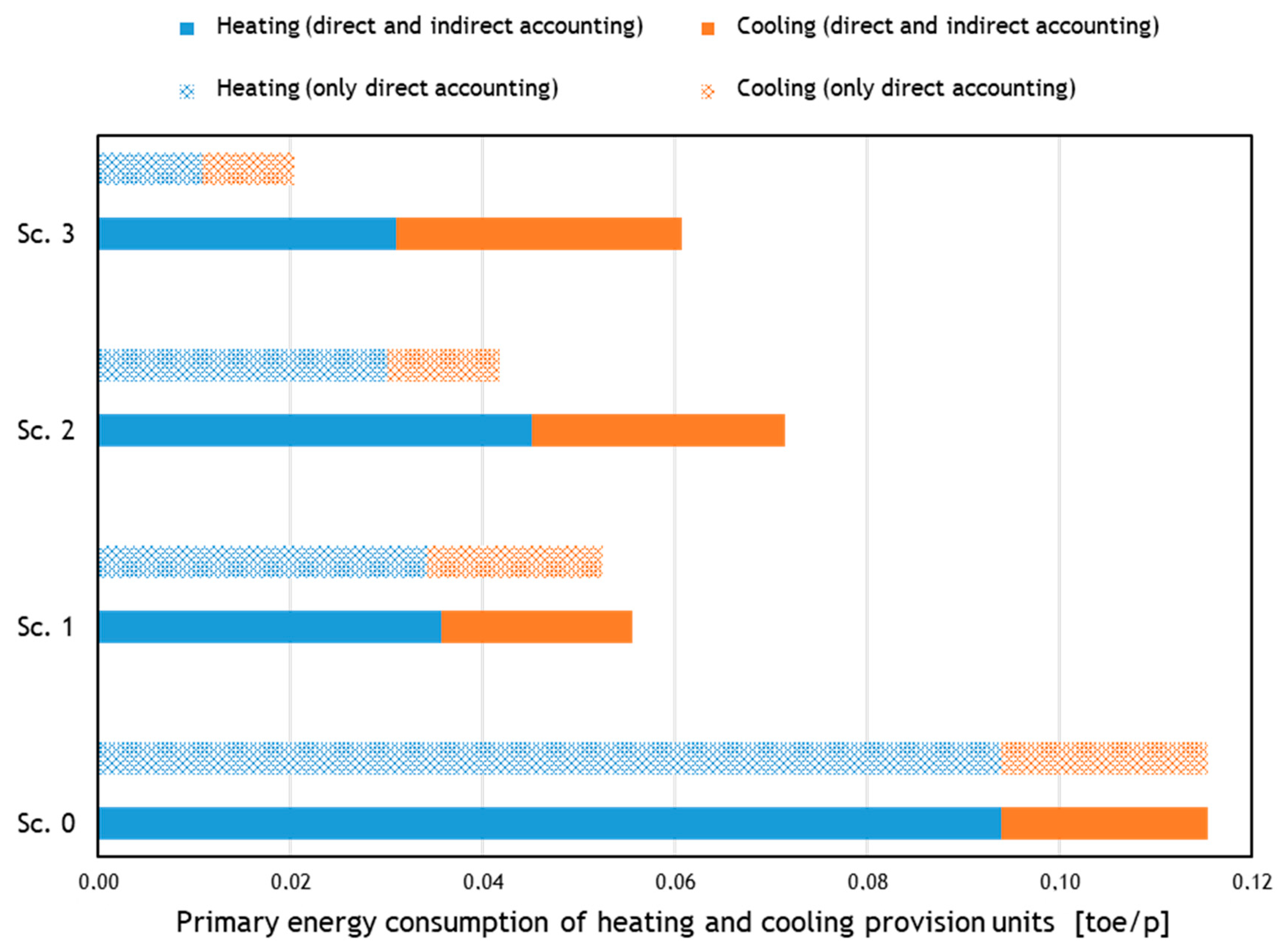
  • The methodology enables policymakers to evaluate end-use efficiency interventions, considering not only direct energy savings but also indirect primary energy consumption. Different efficiency improvements made in the application case demonstrated the relevance of indirect energy consumption through the goods and services involved in such interventions, compared to direct energy savings in household demand. Scenario 1 (equipment improvement) saves 52% with respect to the base case, Scenario 2 (insulation) saves 38% and Scenario 3 (Scenarios 1+2 together) saves 47%. Particularly, savings caused by insulation have significant indirect effects that cannot be ignored.
Information provided by the proposed methodology could support the definition of energy efficiency policies:
  • The gap between real and defined provision unit values could be adopted as an indicator of energy poverty, energy well-being or even energy splurge in a certain city.
  • Separate values of context efficiency and equipment efficiency could be useful for deciding whether to encourage appliance replacement or building quality improvement in a city-level approach.
  • Primary energy consumption of heating and cooling provision units may be established as an indicator of the entire sustainability of heating and cooling services.
In view of the outcomes of this research, some possible future developments can be identified. Firstly, the definition of provision units for other uses within the same conceptual framework. Secondly, the assessment of effects on primary energy consumption due to the implementation of efficiency policies in intermediate sectors (i.e., industry).

Author Contributions

Conceptualization, R.G.S., M.V.R. and E.C.; methodology, R.G.S. and M.V.R.; software, R.G.S.; validation, M.V.R., and E.C.; formal analysis, R.G.S. and M.V.R.; investigation, R.G.S.; resources, R.G.S.; data curation, R.G.S.; writing—original draft preparation, R.G.S.; writing—review and editing, M.V.R.; visualization, R.G.S.; supervision, M.V.R. and E.C. All authors have read and agreed to the published version of the manuscript.

Funding

This research received no external funding.

Conflicts of Interest

The authors declare no conflict of interest.

Nomenclature

Symbols
P U provision unit, k W h / p
c z climatic zone condition, k W h / m 2
c comfort condition
s e socio-economic condition, m 2 / p
D days of heating or cooling
M months of heating or cooling
N population
A building floor area, m 2
a fraction of conditioned floor area
O building occupancy, p
θ temperature, ° C
ε building archetype generic parameter
ρ positive value as small as desired
E energy, k W h t o e
f p primary energy conversion factor
η efficiency
C F coverage factor
D matrix of commodity output proportions
B matrix of industry input proportions
e exogenous vector of final demand, monetary units
x total output vector of each industry, monetary units
q total output vector of each commodity, monetary units
I identity matrix
R exogenous resource vector, t o e
R C B consumption-based approach exogenous resource consumption vector, t o e
λ fraction of provision unit obtained from certain secondary energy
p relative household demand of commodity
e total final household demand of commodity, monetary units
T time horizon of interventions, years
c intervention cost distribution for each commodity, monetary units
β share of secondary energy
A building archetype floor area, m 2
e . S building archetype transparent envelope area, m 2
U building archetype opaque average envelope transmittance, W / m 2 K
U w building archetype transparent average envelope transmittance, W / m 2 K
α building archetype opaque envelope average absorption coefficient
b building archetype adjustment factor
Subscripts
0 reference
p r i m primary
s e c secondary
u useful
o b j defined
h heating
c cooling
e equipment
c context
h h household
g a s gas
e l electricity
Acronyms
CBAConsumption-based approach
COPCoefficient of performance
HVACHeating, ventilation and air conditioning
IEAInternational Energy Agency
INDECNational Institute of Statistics and Census of Argentina
IRAMArgentine Institute for Standardization and Certification
IOInput–Output
IOAInput–Output analysis
MRIOMulti-Regional Input–Output Model
PBAProduction-based approach
SUTsSupply and Use tables

Appendix A. Simplified Method for Climatic Zone Condition Calculation

A simplified method for determining the climatic zone conditions for heating and cooling, c z h ; c z c , is presented in this paragraph. This method is based on a simplified application of the ISO 13790:2008 and IRAM 11900:2017 procedures [18,61], and considers specific thermal parameters of buildings (Table 1). It can be adopted in the absence of official energy labeling software or procedures and when seeking a simple first evaluation as well.
Firstly, the specific heat transfer coefficients for heating and cooling periods, respectively, H h ; H c ( W / m 2 K ), must be calculated according to Expression (A1),
H h = H t r + H inf ; h H c = H t r + H inf ; c
where H i n f ; h and H i n f ; c are the specific ventilation heat transfer coefficients for heating and cooling periods, respectively, (as defined in Table 1) and H t r is the specific transmission heat transfer coefficient, calculated according to Expression (A2), considering thermal building-specific parameters ( S / A ; U ; U w ; b ; e ) defined in Table 1.
H t r = [ U b ( 1 e ) + U w e ] S / A
Once the specific heat transfer coefficients have been established, it is possible to calculate the monthly thermal energy need for the i-th month Q u ; h ; i ; Q u ; c ; i ( k W h / m 2 ) for heating and cooling. The monthly specific thermal energy need (i.e., specific thermal energy that must be added in the heating period or extracted in the cooling period) in the i-th month is determined by Expression (A3),
Q u ; h ; i = ( Q t r inf ; h ; i + Q r a d ; i ) η h ; i Q g r ; i Q u ; c ; i = Q g r ; i η c ; i ( Q t r inf ; c ; i + Q r a d ; i )
where
Q t r i n f ; h ; i is the specific heat transfer by transmission and ventilation/infiltration for the i-th month ( k W h / m 2 ) (heating period), determined according to (A4);
Q t r i n f ; c ; i is the specific heat transfer by transmission and ventilation/infiltration for the i-th month ( k W h / m 2 ) (cooling period), obtained by Expression (A4);
Q r a d ; i is the specific heat transfer due to thermal radiation to the sky for the i-th month ( k W h / m 2 ), determined using Expression (A5);
Q g r ; i is the specific heat gain due to solar radiation for the i-th month ( k W h / m 2 ), determined by means of Expression (A6);
η g r ; h ; i is the dimensionless gain utilization factor for the i-th month (heating period), determined according to (A7);
η g r ; c ; i is the dimensionless loss utilization factor for the i-th month (cooling period), determined according to (A7).
  • Specific heat transfer by transmission and ventilation/infiltration for the i-th month is calculated according to Expression (A4)
    Q t r inf ; h ; i = 24 10 3 H h ( θ c o n f ; h θ e x t ; i ) D i Q t r inf ; c ; i = 24 10 3 H c ( θ c o n f ; c θ e x t ; i ) D i
    where
H h ; H c are the specific heat transfer coefficients for heating and cooling periods, respectively (A1);
θ c o n f ; h ; θ c o n f ; c are the comfort temperatures (i.e., set-point temperatures) for heating and cooling periods, respectively;
θ e x t ; i is the temperature of the external environment (i.e., ambient temperature) of the i-th month;
D i is the number of days of the heating and cooling periods defined for the considered climate.
  • Specific heat transfer due to thermal radiation to the sky of the i-th month is calculated according to Expression (A5)
    Q r a d ; i = 24 10 3 H t r F v R s e h r a d Δ θ s k y D i
    where
H t r is the specific transmission heat transfer coefficient (A2);
F v is a dimensionless form factor for radiation between the building’s envelope surface and the sky; a value of 0.75 is adopted (as an intermediate value between 0.5 for vertical surfaces and 1 for horizontal surfaces);
R s e is the external surface heat resistance of the building envelope, the value assumed is 0.04   m 2 K / W ;
h r a d is the external radiative heat transfer coefficient, adopted 4.45   W / m 2 K ;
Δ θ s k y is the average difference between the external air temperature and the apparent sky temperature, adopted as 11   ° C , as specified in ISO 13790:2008;
D i is the number of days of the heating and cooling periods defined for the considered climate.
  • Specific heat gain due to solar radiation of the i-th month is calculated according to expression (A6)
    Q g r ; i = 24 10 3 S / A [ U b R s e α ( 1 e ) + τ e ] I i D i
    where
S / A ; U ; b ; α ; e ; g are the building’s specific thermal parameters (Table 1);
I i is the solar radiation in the horizontal plane of the i-th month for the considered climate ( W / m 2 ).
  • Gain utilization factor η h ; i and loss utilization factor η c ; i of the i-th month are given by Expression (A7)
    η h ; i = { 1 γ i a h 1 γ i ( a h + 1 ) i f γ i > 0 a n d γ i 1 a h a h + 1 i f γ i = 1 η c ; i = { 1 γ i a c 1 γ i ( a c + 1 ) i f γ i > 0 a n d γ i 1 a c a c + 1 i f γ i = 1 .
    where γ i is the relation between gains and losses for the i-th month according to Expression (A8) and a h and a c are dimensionless parameters that consider the time response of the building, according to Expression (A9)
    γ i = Q g r ; i Q t r inf ; i + Q r a d ; i
    a h = a h ; 0 + τ h τ h ; 0 a c = a c ; 0 + τ c τ c ; 0
In Expression (A9), τ c and τ h are the building’s time constants (Table 1) and a h ; 0 = 0.4 ; τ h ; 0 = 11 h ; a c ; 0 = 0 ; τ c ; 0 = 30 h are adjustment parameters [56].
Finally, Expression (A10) determines the heating and cooling climatic zone conditions c z h ; c z c
c z h = i = 1 M h Q u ; h ; i c z c = i = 1 M c Q u ; c ; i
where
Q u ; h ; i ; Q u ; c ; i are the monthly thermal energy needs for the i-th month, according to expression (A3);
M h ; M c are the number of months of the heating and cooling periods, respectively, for the considered climate.

Appendix B. Detailed Reference Data and Assumptions

Complementary reference data and assumptions not provided in the main text are presented in this section.

Appendix B.1. Building Archetype-Specific Thermal Parameter Definition

The building archetype consists in an abstract entity that enables an energy requirement calculation. The calculation was done by adopting specific thermal parameters, whose values are reported in Table A1.
Table A1. Building archetype-specific thermal parameters and adopted values.
SymbolUnitDescriptionValue
S / A m 2 / m 2 envelope—floor area ratio3.25
b -average adjustment factor that consider the temperature of adjacent zones0.69
U W / m 2 K opaque envelope average transmittance2.12
U w W / m 2 K transparent envelope average transmittance4.90
e -percentage of transparent envelope over total0.04
α -opaque envelope average absorption coefficient0.69
g -transparent envelope average transmission coefficient0.80
H inf ; h W / m 2 K specific ventilation heat transfer coefficient for heating period0.30
H inf ; c W / m 2 K specific infiltration heat transfer coefficient for cooling period1.80
τ h h heating building time constant10.07
τ c h cooling building time constant7.72

Appendix B.2. Climatic Zone Characteristics

The main climatic zone characteristics for the building thermal calculations for the analyzed locations are reported in Table A2. The values of monthly average outdoor temperature θ e x t , i ( ° C ), monthly average solar irradiance in the horizontal plane I i ( W / m 2 ) and cooling (C) or heating (H) days D i for each month are provided.
Table A2. Climatic zone main variables (source: National Building Energy Certification Software Database [18]).
RosarioMendozaBarilocheTucumánBuenos Aires
Month D i θ e x t , i I i D i θ e x t , i I i D i θ e x t , i I i D i θ e x t , i I i D i θ e x t , i I i
° C W / m 2 ° C W / m 2 ° C W / m 2 ° C W / m 2 ° C W / m 2
JanuaryC3125289C3126250-014.5298C3124.6243C3124.7274
FebruaryC2823.6252C2824.1241-014.9268C2823.6224C2823.8238
MarchC1521.6208C1521.5226H3112.2199C3122.5215C1522193
April-017.5158-016.7182H308.6134-019179-018.7140
MayH1513.8123H1512.5147H315.584-018.6146H1515.3105
JuneH301199H309.2124H303.658H3013.2132H3011.987
JulyH3110120H318.6142H312.774H3112.2155H3111.393
AugustH3112150H3111.4178H312.8103H3115.2191H3112.3139
SeptemberH1515187H1514.7210H305.3167-018.6221H1515.2166
October-018.5233-018.9252H317.4227-021.7238-017.7210
NovemberC1521.5285C1520.6258H309.9280C3023.2235C1521.3258
DecemberC3123.6293C3123.7265-012.4297C3126239C3123.8276

Appendix B.3. Specific Thermal Parameters of the Average Building

Average building-specific thermal parameters in the analyzed cities are shown in Table A3. Values were obtained from the National Building Energy Certification Database [18].
Table A3. Specific thermal parameters of the average building in the analyzed cities.
SymbolUnitRosarioMendozaBarilocheTucumánBuenos Aires
S / A m 2 / m 2 3.883.854.013.873.98
b -0.560.550.610.520.52
U W / m 2 K 1.902.081.051.841.86
U w W / m 2 K 4.744.864.005.044.11
e -0.050.070.060.040.05
α -0.650.730.610.750.69
τ -0.810.800.750.810.78
H inf ; h W / m 2 K 0.420.350.240.340.38
H inf ; c W / m 2 K 3.352.811.792.323.52
τ h h 21.3314.5716.3015.4618.34
τ c h 12.429.999.269.449.95

Appendix B.4. National Average Building-Specific Thermal Parameters for Considered Scenarios

Table A4 reports the national average building-specific thermal parameters (Scenarios 0 and 1) and parameters after envelope intervention (Scenarios 2 and 3).
Table A4. National average building-specific thermal parameters for the considered improvement scenarios.
SymbolUnitScenarios 0 and 1Scenarios 2 and 3
S / A m 2 / m 2 3.913.91
b -0.540.54
U W / m 2 K 1.870.53
U w W / m 2 K 4.624.62
e -0.050.05
α -0.690.69
τ -0.780.78
H inf ; h W / m 2 K 0.370.37
H inf ; c W / m 2 K 3.213.21
τ h h 18.0237.23
τ c h 10.1514.31

Appendix B.5. Input–Output Final Demand Variation Commodities

Household final demand variation commodities involved in interventions are reported in Table A5. Scenario 1 consists of equipment efficiency improvement and energy carrier substitution, replacing heating gas systems by high COP heat pumps and upgrading cooling system COPs. Scenario 2 consists of context efficiency improvement by wall and ceiling insulation, while Scenario 3 considers Scenarios 1 and 2 together. In all cases, material costs, labor costs (installation) and financial services were considered.
Table A5. Commodity final demand variation ( Δ e k ) due to improvement scenarios in millions of dollars per year.
CommoditiesScenario 1Scenario 2Scenario 3
HeatingCoolingHeatingCoolingHeatingCooling
Transmission and distribution services (158)981−103−95−337218−391
Gas distribution services through mains (159)−1135-−772-−1135-
Household appliances and parts (122)11001100--11001100
Other plastic products (87)--352352352352
Financial intermediation (161)220220352352572572
Maintenance and repair services (179)1981987070268268

Appendix C. Complete Numerical Results

Complementary results not provided in the main text are shown in this section.

Appendix C.1. Sensitivity Analysis

The numerical results of sensitivity analysis on the values of defined heating and cooling provision unit ratios compared with the reference one, P U o b j / P U o b j , 0 , are reported in Table A6. The modified parameters were: floor area A , transparent envelope area e . S , opaque envelope average transmittance U , transparent envelope average transmittance U w , opaque envelope average absorption coefficient α and average adjustment factor b ; considering ± 25% of input deviations in all cases.
Table A6. Sensitivity analysis of defined provision unit ratios compared with the reference one, P U o b j / P U o b j , 0 , with respect to building archetype parameters.
ParameterUnitValueHeating (%)Cooling (%)
MendozaBarilocheTucumánBuenos AiresMendozaTucumánBuenos Aires
A 80.00−0.43−0.23−1.11−0.451.180.691.18
m 2 64.000.000.000.000.000.000.000.00
48.00−0.110.140.19−0.851.680.001.68
e . S 10.000.170.27−0.65−0.041.420.481.42
m 2 8.000.000.000.000.000.000.000.00
6.000.000.700.000.002.42−0.412.42
U 2.650.241.92−0.850.210.490.720.49
W / m 2 K 2.120.000.000.000.000.000.000.00
1.590.967.122.96−0.380.84−0.983.86
U w 6.13−0.360.45−0.42−0.150.000.002.53
W / m 2 K 4.900.000.000.000.000.000.000.00
3.68−0.48−0.33−1.19−0.820.31−0.360.31
α 0.750.22−0.100.26−0.701.51−0.041.51
0.600.000.000.000.000.000.000.00
0.45−0.140.35−1.04−0.10−0.88−0.910.44
b 0.86−0.361.82−1.45−0.152.110.002.11
-0.690.000.000.000.000.000.000.00
0.520.22−2.834.71−0.704.04−0.254.04

Appendix C.2. Extended Energy Balance

The main results of the extension of traditional energy balance towards energy services are reported in Table A7. Useful energy consumption, context efficiency, real provision units, defined provision units and coverage factors for the five analyzed cities are shown.
Table A7. Useful energy, context efficiency, real provision units, defined provision units and coverage factors in the analyzed cities.
RosarioMendozaBarilocheTucumánBuenos Aires
Heating
Useful energy consumption ( E u ; h ) kWh / p 1492161152145871318
Heating context efficiency ( η c ; h )-1.131.021.381.051.18
Real heating provision unit ( P U h ) kWh / p 1691165171886171556
Defined heating provision unit ( P U h ; o b j ) kWh / p 1542169361077331636
Heating coverage factor ( C F h )-1.100.971.180.840.95
Cooling
Useful energy consumption ( E u ; c ) kWh / p 798599-6661307
Cooling context efficiency ( η c ; c )-2.071.70-2.321.82
Real cooling provision unit ( P U c ) kWh / p 16581019-15462380
Defined cooling provision unit ( P U c ; o b j ) kWh / p 816696-697851
Cooling coverage factor ( C F c )-2.031.46-2.222.80

Appendix C.3. Primary Energy Consumption Accounting

Differences in primary energy consumption, E p r i m , of real heating and cooling provision units due to impact accounting criteria are reported in Table A8 for the three improvement scenarios.
Table A8. Differences in primary energy consumption depending on two different impact accounting criteria in the analyzed improvement scenarios: (a) direct impact accounting and (b) both direct and indirect impact accounting.
Scenario 0Scenario 1Scenario 2Scenario 3
HeatingCoolingHeating CoolingHeatingCoolingHeatingCooling
Only dirtABLEect accounting
Primary energy consumption ( E ˜ p r i m ) toe / p 0.09400.02140.03420.01830.03010.01160.01090.0095
Total ( E ˜ p r i m = E ˜ p r i m , h + E ˜ p r i m , c ) toe / p 0.11540.05250.04170.0204
Direct and indirect accounting
Primary energy consumption ( E ˜ p r i m ) toe / p 0.09400.02140.03570.01990.04520.02630.03110.0297
Total ( E ˜ p r i m = E ˜ p r i m , h + E ˜ p r i m , c ) toe / p 0.11540.05560.07150.0608
Difference
Primary energy consumption ( E ˜ p r i m ) % 0.000.004.398.7550.17126.72185.32212.63
Total ( E ˜ p r i m = E ˜ p r i m , h + E ˜ p r i m , c ) % 0.005.9071.46198.04

References

  1. International Energy Agency. 2018 World Energy Outlook: Executive Summary. Available online: https://www.iea.org/reports/world-energy-outlook-2018 (accessed on 10 November 2019).
  2. Jonsson, D.K.; Gustafsson, S.; Wangel, J.; Höjer, M.; Lundqvist, P.; Svane, Ö. Energy at your service: Highlighting energy usage systems in the context of energy efficiency analysis. Energy Effic. 2011, 4, 355–369. [Google Scholar] [CrossRef]
  3. Cullen, J.M.; Allwood, J.M. Theoretical efficiency limits for energy conversion devices. Energy 2010, 35, 2059–2069. [Google Scholar] [CrossRef]
  4. Cullen, J.M.; Allwood, J.M. The efficient use of energy: Tracing the global flow of energy from fuel to service. Energy Policy 2010, 38, 75–81. [Google Scholar] [CrossRef]
  5. Murray-Leach, R. The World’s First Fuel: How Energy Efficiency Is Reshaping Global Energy Systems; Energy Efficiency Council: Melbourne, Australia, 2019. [Google Scholar]
  6. International Energy Agency. Energy Efficiency Indicators: Fundamentals on Statistics; International Energy Agency: Paris, France, 2014.
  7. European Union. Manual for statistics on energy consumption in households. In Manuals and Guidelines—Environment and Energy; European Union: Luxembourg, 2013; ISBN 9789279330070. [Google Scholar]
  8. International Energy Agency. Energy Efficiency Indicators Highlights, 2017 ed.; International Energy Agency: Paris, France, 2017. [CrossRef]
  9. Hunt, L.C.; Ryan, D.L. Economic modelling of energy services: Rectifying misspecified energy demand functions. Energy Econ. 2015, 50, 273–285. [Google Scholar] [CrossRef] [Green Version]
  10. Wood, R.; Lenzen, M.; Suh, S. Handbook of Input-Output Economics in Industrial Ecology; Springer: Berlin/Heidelberg, Germany, 2009. [Google Scholar]
  11. Ministerio de Energía y Minería. Escenarios Energéticos 2030; Ministerio de Energía y Minería: Buenos Aires, Argentina, 2017.
  12. Ministerio de Desarrollo Productivo. Balances Energéticos. Argentina.gob.ar. 2018. Available online: https://www.argentina.gob.ar/produccion/energia/hidrocarburos/balances-energeticos (accessed on 21 March 2020).
  13. Bienestar Mediante Un Megc, A.D.E.; Mastronardi, L.J.; Mayer, M.N. Quita de subsidios a la energía en Argentina: Análisis de bienestar mediante un MEGC. IDEAS 2015, 32, 47–71. [Google Scholar]
  14. Presidencia de la Nación Decreto 140/2007. Programa Nacional de Uso Racional y Eficiente de la Energía; Boletín of la República Argentina: Buenos Aires, Argentina, 2007. Available online: https://www.boletinoficial.gob.ar (accessed on 21 March 2020).
  15. Zabaloy, M.F.; Recalde, M.; Guzowski, C. Are energy efficiency policies for household context dependent? A comparative study of Brazil, Chile, Colombia and Uruguay. Energy Res. Soc. Sci. 2019, 52, 41–54. [Google Scholar] [CrossRef]
  16. Stagnitta, R.; Abalone, R.; Gastón, A. Modelo analítico para estimar el consumo energético de viviendas en régimen dinámico. Parte 1: Análisis del flujo de energía a través de muros. Av. Energ. Renov. Medio Ambient. 2017, 21, 167–178. [Google Scholar]
  17. González, A.D. Energy Subsidies in Argentina Lead to Inequalities and Low Thermal Efficiency. Energies 2009, 2, 769. [Google Scholar] [CrossRef] [Green Version]
  18. SGE Aplicativo Nacional de Etiquetado de Viviendas. Secr. Gob. Energía. Pres. Nación. 2018. Available online: https://etiquetadoviviendas.energia.gob.ar (accessed on 6 March 2020).
  19. Irrek, W.; Thomas, S. Defining Energy Efficiency. Available online: https://wupperinst.org/fa/redaktion/downloads/misc/energy_efficiency_definition.pdf (accessed on 6 March 2020).
  20. Oikonomou, V.; Becchis, F.; Steg, L.; Russolillo, D. Energy saving and energy efficiency concepts for policy making. Energy Policy 2009, 37, 4787–4796. [Google Scholar] [CrossRef]
  21. Patterson, M.G. What is energy efficiency? Energy Policy 1996, 24, 377–390. [Google Scholar] [CrossRef]
  22. Tanaka, K. Assessment of energy efficiency performance measures in industry and their application for policy. Energy Policy 2008, 36, 2887–2902. [Google Scholar] [CrossRef]
  23. Haas, R. Energy efficiency indicators in the residential sector. Energy Policy 1997, 25, 789–802. [Google Scholar] [CrossRef]
  24. Pérez-Lombard, L.; Ortiz, J.; Velázquez, D. Revisiting energy efficiency fundamentals. Energy Effic. 2012, 6, 239–254. [Google Scholar] [CrossRef]
  25. International Energy Agency. World Energy Statistics 2018. Available online: https://www.iea.org/reports (accessed on 6 March 2020).
  26. Schipper, L.; Unander, F.; Murtishaw, S.; Ting, M. Indicators of Energy Use and Carbon Emissions: Explaining the Energy Economy Link. Annu. Rev. Energy Environ. 2001, 26, 49–81. [Google Scholar] [CrossRef]
  27. Odyssee-Mure Energy Efficiency Trends and Policies in the EU 27. Energy 2009. Available online: https://www.odyssee-mure.eu (accessed on 6 March 2020).
  28. Fell, M. Energy services: A conceptual review. Energy Res. Soc. Sci. 2017, 27, 129–140. [Google Scholar] [CrossRef]
  29. Kalt, G.; Wiedenhofer, D.; Görg, C.; Haberl, H. Conceptualizing energy services: A review of energy and well-being along the Energy Service Cascade. Energy Res. Soc. Sci. 2019, 53, 47–58. [Google Scholar] [CrossRef]
  30. Sorrell, S. Reducing energy demand: A review of issues, challenges and approaches. Renew. Sustain. Energy Rev. 2015, 47, 74–82. [Google Scholar] [CrossRef] [Green Version]
  31. Modi, V.; McDade, S.; Lallement, D.; Saghir, J. Energy Services for the Millennium Development Goals; World Bank: Washington, DC, USA, 2005. [Google Scholar]
  32. Fouquet, R. Energy Services. In The New Palgrave Dictionary of Economics; Palgrave Macmillan: London, UK, 2018. [Google Scholar]
  33. Sovacool, B.K. Conceptualizing urban household energy use: Climbing the “Energy Services Ladder”. Energy Policy 2011, 39, 1659–1668. [Google Scholar] [CrossRef]
  34. Cravioto, J.; Yamasue, E.; Okumura, H.; Ishihara, K.N. Energy service satisfaction in two Mexican communities: A study on demographic, household, equipment and energy related predictors. Energy Policy 2014, 73, 110–126. [Google Scholar] [CrossRef]
  35. Nakićenović, N.; John, A. CO2 reduction and removal: Measures for the next century. Energy 1991, 16, 1347–1377. [Google Scholar] [CrossRef] [Green Version]
  36. Nakićenović, N.; Gilli, P.V.; Kurz, R. Regional and global exergy and energy efficiencies. Energy 1996, 21, 223–237. [Google Scholar] [CrossRef]
  37. Grübler, A.; Nakićenović, N.; Victor, D.G. Dynamics of energy technologies and global change. Energy Policy 1999, 27, 247–280. [Google Scholar] [CrossRef] [Green Version]
  38. Flórez-Orrego, D.; Da Silva, J.A.M.; de Oliveira, S., Jr. Exergy and environmental comparison of the end use of vehicle fuels: The Brazilian case. Energy Convers. Manag. 2015, 100, 220–231. [Google Scholar] [CrossRef]
  39. Reistad, G.M. Available Energy Conversion and Utilization in the United States. J. Eng. Power 1975, 97, 429–434. [Google Scholar] [CrossRef]
  40. Wall, G. Exergy conversion in the Swedish society. Resour. Energy 1987, 9, 55–73. [Google Scholar] [CrossRef] [Green Version]
  41. Kümmel, R.; Strassl, W.; Gossner, A.; Eichhorn, W. Technical progress and energy dependent production functions. J. Econ. 1985, 45, 285–311. [Google Scholar] [CrossRef]
  42. Ayres, R.U. The minimum complexity of endogenous growth models: The role of physical resource flows. Energy 2001, 26, 817–838. [Google Scholar] [CrossRef]
  43. Ayres, R.U.; Warr, B. Accounting for growth: The role of physical work. Struct. Chang. Econ. Dyn. 2005, 16, 181–209. [Google Scholar] [CrossRef]
  44. Warr, B.; Ayres, R. REXS: A forecasting model for assessing the impact of natural resource consumption and technological change on economic growth. Struct. Chang. Econ. Dyn. 2006, 17, 329–378. [Google Scholar] [CrossRef]
  45. Serrenho, A.C.; Warr, B.; Sousa, T.; Ayres, R.U.; Domingos, T. Structure and dynamics of useful work along the agriculture-industry-services transition: Portugal from 1856 to 2009. Struct. Chang. Econ. Dyn. 2016, 36, 1–21. [Google Scholar] [CrossRef]
  46. Brockway, P.E.; Barrett, J.R.; Foxon, T.J.; Steinberger, J.K. Divergence of Trends in US and UK Aggregate Exergy Efficiencies 1960–2010. Environ. Sci. Technol. 2014, 48, 9874–9881. [Google Scholar] [CrossRef] [PubMed]
  47. Sciubba, E. Beyond thermoeconomics? The concept of Extended Exergy Accounting and its application to the analysis and design of thermal systems. Exergy Int. J. 2001, 1, 68–84. [Google Scholar] [CrossRef]
  48. Sciubba, E. Exergo-economics: Thermodynamic foundation for a more rational resource use. Int. J. Energy Res. 2005, 29, 613–636. [Google Scholar] [CrossRef]
  49. Rocco, M.V.; Colombo, E.; Sciubba, E. Advances in exergy analysis: A novel assessment of the Extended Exergy Accounting method. Appl. Energy 2014, 113, 1405–1420. [Google Scholar] [CrossRef]
  50. Kratena, K. From ecological footprint to ecological rent: An economic indicator for resource constraints. Ecol. Econ. 2008, 64, 507–516. [Google Scholar] [CrossRef] [Green Version]
  51. Miller, R.E.; Blair, P.D. Input-Output Analysis; Cambridge University Press: Cambridge, UK, 2009. [Google Scholar]
  52. Chen, S.; Chen, B. Urban energy consumption: Different insights from energy flow analysis, input-output analysis and ecological network analysis. Appl. Energy 2015, 138, 99–107. [Google Scholar] [CrossRef]
  53. Liu, Z.; Geng, Y.; Lindner, S.; Zhao, H.; Fujita, T.; Guan, D. Embodied energy use in China’s industrial sectors. Energy Policy 2012, 49, 751–758. [Google Scholar] [CrossRef]
  54. Rocco, M.V.; Ferrer, R.J.F.; Colombo, E. Understanding the energy metabolism of World economies through the joint use of Production- and Consumption-based energy accountings. Appl. Energy 2018, 211, 590–603. [Google Scholar] [CrossRef]
  55. Owen, A.; Brockway, P.E.; Correa, L.I.B.; Bunse, L.; Sakai, M.; Barrett, J. Energy consumption-based accounts: A comparison of results using different energy extension vectors. Appl. Energy 2017, 190, 464–473. [Google Scholar] [CrossRef]
  56. Hong, J.; Shen, G.Q.; Guo, S.; Xue, F.; Zheng, W. Energy use embodied in China’s construction industry: A multi-regional input-output analysis. Renew. Sustain. Energy Rev. 2016, 53, 1303–1312. [Google Scholar] [CrossRef] [Green Version]
  57. Zhang, Y.; Zheng, H.; Yang, Z.; Su, M.; Liu, G.; Li, Y. Multi-regional input-output model and ecological network analysis for regional embodied energy accounting in China. Energy Policy 2015, 86, 651–663. [Google Scholar] [CrossRef]
  58. Rocco, M.V.; Colombo, E. Evaluating energy embodied in national products through Input-Output analysis: Theoretical definition and practical application of international trades treatment methods. J. Clean. Prod. 2016, 139, 1449–1462. [Google Scholar] [CrossRef]
  59. Heun, M.K.; Owen, A.; Brockway, P.E. A physical supply-use table framework for energy analysis on the energy conversion chain. Appl. Energy 2018, 226, 1134–1162. [Google Scholar] [CrossRef]
  60. Haas, R.; Nakicenovic, N.; Ajanovic, A.; Faber, T.; Kranzl, L.; Müller, A.; Resch, G. Towards sustainability of energy systems: A primer on how to apply the concept of energy services to identify necessary trends and policies. Energy Policy 2008, 36, 4012–4021. [Google Scholar] [CrossRef]
  61. Standard, E.N. Energy Performance of Buildings—Calculation of Energy Use for Space Heating and Cooling. Available online: http://www.cres.gr/greenbuilding/PDF/prend/set3/WI_14_TC-draft-ISO13790_2006-07-10.pdf (accessed on 15 April 2020).
  62. IRAM 11900. Prestaciones Energéticas en Viviendas. Método de Cálculo. 2017. Available online: http://www.iram.org.ar (accessed on 15 April 2020).
  63. Instituto de Estadísticas y Censos de Argentina Censo. 2010 Argentina resultados definitivos: Mapas. In INDEC. Censo Nac. Población, Hogares y Viviendas 2010; Instituto Geográfico Nacional e INDEC: Buenos Aires, Argentina, 2010. [Google Scholar]
  64. Gastiarena, M.; Gil, S. Gas versus electricidad: Uso de la energía en el sector residencial. Petrotecnia 2017, LVI, 50–60. [Google Scholar]
  65. SGE Balances Energéticos Nacionales. 2016. Available online: https://www.argentina.gob.ar/produccion/energia/hidrocarburos/balances-energeticos (accessed on 20 November 2019).
  66. International Energy Agency. World Energy Balances 2016; OECD: Paris, France, 2016; ISBN 9789264261587.
  67. Lenzen, M.; Moran, D.; Kanemoto, K.; Geschke, A. Building Eora: A Global Multi-Region Input–Output Database at High Country and Sector Resolution. Econ. Syst. Res. 2013, 25, 20–49. [Google Scholar] [CrossRef]
  68. Lenzen, M.; Kanemoto, K.; Moran, D.; Geschke, A. Mapping the Structure of the World Economy. Environ. Sci. Technol. 2012, 46, 8374–8381. [Google Scholar] [CrossRef]
  69. INDEC. Censo Nacional de Población, Hogares y Viviendas 2010—Aspectos Operativos y Metodológicos. Available online: https://redatam.indec.gob.ar/redarg/CENSOS/CPV2010rad/Docs/aspectos.pdf (accessed on 2 November 2019).
Figure 1. Useful energy—provision unit.
Sustainability 12 06563 g001
Figure 2. Provision unit definition: input variables for calculating comfort condition, socio-economic condition, climatic zone condition and building archetype role.
Sustainability 12 06563 g002
Figure 3. Possible situations that could lead to dissimilarities between real consumption and theoretical requirement: differences in provision unit, useful energy or secondary energy.
Sustainability 12 06563 g003
Figure 4. Extension of the energy balance for the j use: secondary energy, useful energy and provision unit.
Sustainability 12 06563 g004
Figure 5. Sensitivity analysis of defined provision unit ratios compared with the reference one ( P U o b j / P U o b j ; 0 ) with respect to building archetype parameters.
Sustainability 12 06563 g005
Figure 6. Defined provision units, real provision units and coverage factors in the analyzed cities.
Sustainability 12 06563 g006
Figure 7. Differences in primary energy consumption depending on two different impact accounting criteria in the analyzed improvement scenarios: (a) direct impact accounting and (b) both direct and indirect impact accounting.
Sustainability 12 06563 g007
Table 1. Building archetype-specific thermal parameters.
SymbolUnitDescription
S / A m 2 / m 2 envelope—floor area ratio
b -average adjustment factor that considers temperature of adjacent zones
U W / m 2 K opaque envelope average transmittance
U w W / m 2 K transparent envelope average transmittance
e -percentage of transparent envelope over total
α -opaque envelope average absorption coefficient
g -transparent envelope average transmission coefficient
H inf ; h W / m 2 K specific ventilation heat transfer coefficient for heating period
H inf ; c W / m 2 K specific infiltration heat transfer coefficient for cooling period
τ h h time constant of the zone for heating period
τ c h time constant of the zone for cooling period
Table 2. Gas and electricity consumption per capita ( k W h / p ) for heating and cooling in the analyzed cities.
RosarioMendozaBarilocheTucumánBuenos Aires
Gas consumption for heating per capita ( E ˜ s e c ; g a s ; h )1863223078106421791
Electricity consumption for heating per capita ( E ˜ s e c ; e l ; h )5332305169
Electricity consumption for cooling per capita ( E ˜ s e c ; e l ; c )267213-205458
Table 3. Construction of the extracted energy vector ( R ) allocating International Energy Agency (IEA) primary energy supply by source data.
IndustryValuePrimary ResourceValue
ktoe ktoe
Extraction of petroleum, gas, coal and uranium78,799Coal823
Crude oil28,068
Oil products3097
Natural gas44,652
Nuclear2159
Oils and oilseed products3379Biofuels and waste3379
Electricity4075Hydro3207
Geothermal, solar, etc.49
Electricity819
Table 4. Context efficiencies, equipment efficiencies and secondary energy shares for the considered improvement scenarios.
Scenario 0Scenario 1Scenario 2Scenario 3
Heating
Context efficiency ( η c ; h )1.131.133.543.54
Gas equipment efficiency ( η e ; g a s ; h )0.73-0.73-
Electrical equipment efficiency ( η e ; e l ; h )2.473.502.473.50
Gas share ( β g a s ; h ) 0.970.000.970.00
Electricity share ( β e l ; h ) 0.031.000.031.00
Cooling
Context efficiency ( η c ; c )2.082.083.993.99
Equipment efficiency ( η e ; c )2.993.502.993.50
Table 5. Defined provision units, components of their definitions and provision unit ratios with the reference one in the analyzed cities.
RosarioMendozaBarilocheTucumánBuenos Aires
Comfort conditions ( c h ; c c )-1.001.001.001.001.00
Socio-economic condition ( s e ) m 2 / p 15.1213.6514.3412.0216.70
Heating
Climatic zone condition ( c z h ) kWh / m 2 1021244266198
Provision unit ( P U h ; o b j ) kWh / p 1542169361077331636
Provision unit ratio with reference ( P U h ; o b j / P U h ; o b j ; 0 )-1.001.103.960.481.06
Cooling
Climatic zone condition ( c z c ) kWh / m 2 5451-5851
Provision unit ( P U c ; o b j ) kWh / p 816696-697851
Provision unit ratio with reference ( P U c ; o b j / P U c ; o b j ; 0 )-1.000.85-0.861.04
Table 6. Context and equipment efficiencies, fractions of provision units obtained from gas and electricity (heating case) and secondary energy shares (heating case) for the analyzed cities.
RosarioMendozaBarilocheTucumánBuenos Aires
Heating
Context efficiency ( η c ; h )1.131.021.381.051.18
Gas equipment efficiency ( η e ; g a s ; h )0.730.690.660.730.69
Electrical equipment efficiency ( η e ; e l ; h )2.472.262.002.301.20
Average equipment efficiency ( η e ; h )0.780.710.670.850.70
Fraction of provision unit obtained from gas ( λ g a s ; h )0.920.960.990.800.94
Fraction of provision unit obtained from electricity ( λ g a s ; h )0.080.040.010.200.06
Gas share ( β g a s ; h )0.970.980.990.920.98
Electricity share ( β e l ; h )0.030.020.010.080.02
Cooling
Context efficiency ( η c ; c )2.071.70-2.321.82
Equipment efficiency ( η e ; c )2.992.82-3.252.85
Table 7. Primary energy consumption of real heating and cooling provision units in the analyzed improvement scenarios.
Scenario 0Scenario 1Scenario 2Scenario 3
HeatingCoolingHeatingCooling HeatingCoolingHeatingCooling
Context efficiency ( η c ) 1.132.081.132.083.543.993.543.99
Useful energy consumption ( E u ) kWh / p 14927981492798477415477415
Equipment efficiency ( η e ) 0.782.993.53.50.782.993.53.5
Gas consumption ( E ˜ s e c ; g a s ) kWh / p 1863-0-596-0-
Electricity consumption ( E ˜ s e c ; e l ) kWh / p 5326742622817139136119
Primary energy consumption ( E ˜ p r i m ) toe / p 0.09400.02140.03570.01990.04520.02630.03110.0297
Total ( E ˜ p r i m = E ˜ p r i m , h + E ˜ p r i m , c ) toe / p 0.11540.05560.07150.0608
Primary energy saving with respect to Scenario 0%0523847

