Economic Convergence in EU NUTS 3 Regions: A Spatial Econometric Perspective

Abstract

The topic of economic convergence is still crucial in the European Union (EU) as promoting regional growth and the reduction of disparities remains a key objective. In this paper we investigate development and economic growth across EU regions. Particular attention is given to σ-convergence and β-convergence. These analyses are carried out for regional units corresponding to the third level of the NUTS (Nomenclature of Territorial Units for Statistics) classification. Focusing on a refined geographical scale could offer a detailed picture of the regional growth dynamics within the EU. Additionally, we use a spatial augmented version of the conditional β-convergence model to take into account the spatial interdependencies among regions. Findings shed light on the impact of spatial interaction effects and on the need of territorial policies to achieve convergence in the EU. This aspect highlights how coordinating the regional development policies between regions is pivotal to achieve economic, as well as social and political stability within the EU.

1. Introduction

The presence of regional disparities across European Union (EU) regions, strengthened by the global financial crisis, demands new regional policies that can promote growth and regional equality within countries and across the EU regions [1,2,3,4,5]. The objectives of helping less-developed regions and supporting territorial cooperation have inspired the EU Cohesion policy.

This strategy is the EU’s main investment policy and it should be realized mainly through growth and the reduction of the significant economic, social, and territorial disparities that still exist between European regions and member states. The importance of this objective has not declined over time. Economic, Social, and Territorial Cohesion is basically managed by Title XVIII of the Consolidated Version of the Treaty on the Functioning of the European Union. In particular, Article 174 (ex Article 158 of the Treaty establishing the European Community) states that:

“In order to promote its overall harmonious development, the Union shall develop and pursue its actions leading to the strengthening of its economic, social and territorial cohesion. In particular, the Union shall aim at reducing disparities between the levels of development of the various regions and the backwardness of the least favoured regions. Among the regions concerned, particular attention shall be paid to rural areas, areas affected by industrial transition, and regions which suffer from severe and permanent natural or demographic handicaps such as the northernmost regions with very low population density and island, cross-border and mountain regions.”

Since the launch of the Cohesion Policy, the objective of the reduction of disparities has been re- interpreted in the promotion of economic convergence between EU regions. Therefore, to evaluate a successful application of these policies, it is necessary to analyse in depth the economic growth in European regions.

During the last decades, the convergence problem represented a crucial issue in the regional economic growth debate. Many applied economists have observed that the gross domestic product (GDP) per capita of poor regions tend to converge to those of richer regions. The most popular methodologies in the quantitative measurement of convergence are based on the concepts of $\sigma$-convergence and $\beta$-convergence [6]. The $\sigma$-convergence hypothesis refers to the reduction of disparities between countries or regions and is assessed by measuring dispersion in GDP per capita across a group of economies, over time. The $\beta$-convergence hypothesis implies a negative relationship between the initial level of GDP per capita and the growth rate of GDP per capita, and is assessed by growth regressions (see Section 2). Both the $\sigma$-convergence and the $\beta$-convergence approaches are often based on methods where the geographical characteristics of the data are not considered.

In this paper, our aim is to reconsider the problem of regional economic convergence in Europe, adopting a spatial econometric perspective. Our purpose is to highlight that ignoring the multidirectional dependence among EU neighbouring regions causes a misspecification of the concept of regional convergence. In fact, traditional statistical methods applied in the empirical analysis of regional economic convergence often assume independence among observations. By contrast, such a hypothesis is violated when the analysis involves territorial units, and proximity relationships often imply reciprocal influence. If this circumstance is not considered, and thus standard estimation procedures are applied, the resulting analysis can lead to biased estimates [7].

Our analysis is implemented at NUTS 3 level using a cross-sectional approach [8]. The NUTS (Nomenclature of Territorial Units for Statistics) classification is a hierarchical classification that is divided into three levels, where the NUTS 1 level identifies larger socio-economic regions, the NUTS 2 level indicates basic regions, often considered in the definition of regional policies, and the NUTS 3 level identifies the smaller regions, which can be considered for specific analyses (https://ec.europa.eu/eurostat/web/nuts/background).

NUTS 2 is the most used level for the analysis of the $\beta$-convergence process in EU, while less attention has been devoted to the NUTS 3 level. Some exceptions can be found in recent contributions, focusing on a group of NUTS 3 regions in the EU or on regions belonging to single countries [9,10,11,12]. Some of these contributions considered spatial effects in modelling economic growth at the sub-regional level, assessing the presence of local spatial spillovers as in the case of Italy [10].

Using a finer geographical scale may reveal local spatial effects that are not evident at NUTS 2 level. Besides, this analysis could be relevant from a policy perspective, supporting the definition of place-based measures for the reduction of disparities.

Unfortunately, the analysis of the $\beta$-convergence process at NUTS 3 level presents some problems in terms of data availability. In fact, some variables for the definition of the economic model are not offered at this spatial scale. These variables can be estimated making use of a spatial disaggregation technique that will be summarized in Section 4.

We use data derived from the European regional database by Cambridge Econometrics that is now available free of charge from the new Annual Regional Database of the European Commission’s Directorate General for Regional and Urban Policy (ARDECO, https://ec.europa.eu/knowledge4policy/territorial/ardeco-database_en) maintained by the European Commission’s Joint Research Centre.

The original variables from these two data sets have been transformed according to the definition of the economic models outlined in the next sections.

One of the main contributions of the paper is related to the size of the data sets used that refer to two different time spans. The first considers 901 NUTS 3 EU regions across the period 1981–2014, the second analyses 1133 NUTS 3 EU regions through the years 1991–2014. The two different samples of regions differ essentially since the second one contains also regions belonging to Eastern Europe. In this way, it is possible to evaluate different paths of economic growth of EU regions also after the annexation of countries of Eastern Europe. To the best of our knowledge, this is the most extended cross-sectional analysis of the $\beta$-convergence process in EU regions.

A cross-sectional scheme facilitates the consideration of the variation of phenomena across units in space. The variation over time, captured by a panel data approach [13,14], is beyond our scope. In fact, our analysis is intended to follow the cross-sectional framework that, for the conditional $\beta$-convergence analysis, was introduced by [6]. Furthermore, the cross-sectional analysis is consistent with our aim of capturing long-run transitional dynamics. Conversely, a panel data approach is useful in assessing short-run effects. In fact, while panel data observations are typically based on five-year averages, observations used in cross-sectional analyses are based upon 25-year, or longer, averages (see, among others, [15,16]). As an additional aspect, the use of a cross-sectional analysis facilitates the comparison of our results with findings obtained in other $\beta$-convergence studies, mostly focused on this approach. In fact, with respect to panel data approaches, cross-sectional models have a longer history in the study of regional convergence, and also their spatial econometric transformations are better developed [16].

The layout of the paper is the following. In Section 2, we review the standard concepts of economic convergence. Section 3 concerns the description of the spatial augmented model for the analysis of $\beta$-convergence. Section 4 describes some methodological issues that should be addressed in our study. Section 5 is devoted to the empirical analysis of economic convergence for EU NUTS 3 regions. Section 6 contains some discussions and policy implications. Finally, Section 7 concludes the paper.

2. The Economic Convergence Models

Economic convergence represents one of the most important features of the Neoclassical growth theory [17] and refers to the long-run process where the GDP per capita of poor regions grows more quickly than in the rich ones. This process should lead poor countries to catch up with rich ones across time [18].

The $\sigma$-convergence and $\beta$-convergence represent two well-known approaches for testing the convergence hypothesis [18,19]. The $\sigma$-convergence hypothesis is analysed through the following equation [6]:

$${\sigma }_t^2=\frac{1}{N}{{\displaystyle \sum }}_{i=1}^N{\left(\ln y_{it}-{\overline{x}}_t\right)}^2$$

(1)

where $y_{it}$ is the GDP per capita of the $i$-th regional economy at time $t$, ${\overline{x}}_t$ is the mean of $\ln y_{it}$and $N$ is the number of regional economies studied. In empirical studies, to measure $\sigma$-convergence, the coefficient of variation $CV={\sigma }_t/{\overline{x}}_t$ is often preferred instead of the variance, since ${\sigma }_t^2$ is not useful for comparisons. If there is a decreasing long-term trend of the dispersion, then disparities between countries or regions are reduced and so the$\sigma$-convergence hypothesis is satisfied.

Unfortunately, the$\sigma$-convergence approach is not supported by any economic theory and, additionally, the variance of natural logarithms is insensible to spatial permutations. Note that, following [20], in this paper, we consider $CV$ in its unweighted version, instead of using the version weighted by the regions’ proportions of the national populations. In fact, the unweighted version of $CV$, differently from the weighted form, provides an estimate of regional inequality as requested by the $\sigma$-convergence investigation [20].

The $\beta$-convergence hypothesis is assessed by performing growth regressions. This framework postulates exogenous saving rates and a production function based on decreasing productivity of capital and constant returns [6].

The standard statistical model used to measure $\beta$-convergence is [21]:

$$g_i={\beta }_0+{\beta }_1\ln y_{it-T }+{x^{\prime }}_i\mathsf{\beta }+{\epsilon }_i, {\epsilon }_i\sim N\left(0,{\sigma }^2\right)$$

(2)

where $g_i=\frac{1}{T}\ln \left(\frac{y_{it} }{y_{it-T }}\right)$ is the dependent variable that denotes the average growth rates of GDP per worker for $T$ periods under investigation, $y_{it}$ and $y_{it-T }$ are the GDP per worker at the final time and in the initial period, $x_i^{}$ is the vector of $p$ explanatory variables (i.e., the structural characteristics) available for each spatial unit $i$, $\mathsf{\beta }$ is the associated parameters vector to be estimated, and ${\epsilon }_i$ is the independent and identically distributed error term, with zero mean and variance ${\sigma }^2$. Note that the time $t$ is fixed and $i=1,2,\dots ,N$ represents the cross-sectional dimension (i.e., the spatial units). If the explanatory variables in Equation (2) constitute only the natural logarithm of the initial level of GDP per worker, $\ln y_{it-T }$, (i.e., $p=0$), we are defining a model for the analysis of absolute $\beta$-convergence. Conversely, if $p>0$, Equation (2) describes a conditional $\beta$-convergence model that contains additional variables to control for structural differences [6]. The $\beta$-convergence framework is satisfied if ${\beta }_1$is significant and negative. The paradigm of absolute $\beta$-convergence is considered reasonable only when the economic growth is investigated at an intra-national level [22].

3. The Spatial Augmented Model of Conditional β-Convergence

In Equation (2), regional economies are considered as independent entities, mainly neglecting the role of spatial interaction [23]. This hypothesis is clearly violated in all geographical studies, where “everything is related to everything else, but near things are more related than distant things’’ (Tobler’s first law of geography [24]).

Spatial effects include spatial dependence and spatial heterogeneity [25]. Spatial dependence reveals a situation where observations at one location depend on the values at nearby locations. Spatial heterogeneity indicates instability, over space, of economic variables, and can be displayed in a regression model by non-constant error variances (i.e., heteroscedasticity) or by space-varying coefficients (i.e., structural instability).

In recent decades, many attempts have been made to extend the standard economic convergence analysis to include spatial effects. The US regional income convergence from a spatial econometric perspective is studied in [23]. The convergence processes in the European Union using spatial methods is analysed by [26]. Exploratory spatial data analysis (ESDA) tools are applied to evaluate the importance of geographical position and spatial interactions in [27]. A constrained optimization algorithm for the identification of multiple spatial regimes in EU regions is used by [7], allowing for explicit variation in the parameters of the Solow growth model.

An important contribution [28] addressed the problem of technological interdependence among economies and examined the impact of spillover effects from a theoretical point of view to derive a spatial expansion of the growth equation. Therefore, in this paper, we decided to use the model introduced by these authors in order to verify the presence of $\beta$-convergence. In fact, throughout this framework we take into account both physical capital and spatial externalities in knowledge to model technological progress at NUTS 3 level.

The model proposed by [28] is defined starting from the following Cobb–Douglas production function defined as:

$$Y_{it}=A_{it}{K}_{it}^{{\alpha }_k}{L}_{it}^{1-{\alpha }_k}$$

(3)

where, at time $t$, $Y_{it}$ is the output, $K_{it}$ the level of physical capital, $L_{it}$ the level of labour, and $A_{it}$ the level of technology. The exponent ${\alpha }_k$in (3) expresses the output elasticity with respect to physical capital. The final specification of the statistical model for the analysis of conditional $\beta$-convergence, for units $i$, can be expressed as follows [28]:

$$\begin{array}{l}{g}_i={\beta }_0+{\beta }_1\ln y_{it-T }+{\beta }_2\ln s_i^k+{\beta }_3\ln v_i+\rho {\displaystyle \sum _{j=1 }^N}{w}_{ij}{g}_j+{\rho }_1{\displaystyle \sum _{j=1 }^N}{w}_{ij}\ln y_{jt-T}+{\rho }_2{\displaystyle \sum _{j=1 }^N}{w}_{ij}\\ \hspace{1em}\hspace{1em}\hspace{1em}\hspace{1em}\hspace{1em}\hspace{1em} \ln s_j^k+{\rho }_3{\displaystyle \sum _{j=1 }^N}{w}_{ij}\ln v_j+{\epsilon }_i \end{array}$$

(4)

where $g_i=\frac{1}{T}\ln \left(\frac{y_{it} }{y_{it-T }}\right)$denotes the average of GDP per worker growth rate, $T$ expresses the number of periods under investigation, $w_{ij}$ is the entry of the contiguity matrix $W$ that measures the proximity between the regional economy$i$ and its neighboring economies $j\mathrm{s}$, the variable $s_i^k$ represents the saving rate of physical capital, and $v_i=n_i+l+k$, with $n_i$ as the working population growth rate, $l$ is the rate of technological progress, $k$ indicates the depreciation rate of capital. Following [26], the parameters in (4) can be specified as follows: ${\beta }_0$ is a constant, ${\beta }_1=-\frac{1-e^{-\lambda T}}{T}$, ${\beta }_2=-{\beta }_3=\frac{{\alpha }_k+{\varphi }_k}{1-{\alpha }_k-{\varphi }_k}\frac{1-e^{-\lambda T}}{T}$, ${\rho }_1=\frac{\zeta \left(1-{\alpha }_k\right)}{1-{\alpha }_k-{\varphi }_k}\frac{1-e^{-\lambda T}}{T}$, ${\rho }_3=-{\rho }_2=\frac{\zeta {\alpha }_k}{1-{\alpha }_k-{\varphi }_k}\frac{1-e^{-\lambda T}}{T}$ and $\rho =\frac{\zeta \left(1-{\alpha }_k\right)}{1-{\alpha }_k-{\varphi }_k}$. In model (4), the level of technology of a certain economy is linked to the level of physical capital, with ${\varphi }_k$ being the parameter describing the strength of these externalities, and depending on also the level of technology of neighbouring economies, with the parameter $\zeta$ that controls for these spatial externalities.

The model (4) theoretically ensures convergence since the growth of GDP per worker is a negative function of the initial level of GDP per worker (i.e., ${\beta }_1$is negative), but only after controlling for the other structural characteristics of the steady state (i.e., the covariates of the model). Moreover, the GDP per worker depends also, in the same direction, on the same spatially lagged variables because of the technological interdependence and spatial externalities. Finally, the term $\rho {\sum }_{j=1 }^N{w}_{ij}{g}_j$ shows that the GDP per worker growth rate of country $i$ positively depends on the growth rate observed for its neighboring regions.

The model specification (4) corresponds to the spatial Durbin model (SDM). The SDM specification subsumes as special cases both the spatial lag model and the spatial error model (SEM), which have been widely used in previous empirical studies on economic growth [29,30]. The use of the SDM was encouraged by [30] also from the statistical point of view. This suggestion is based on the plausibility of two different circumstances that it is possible to find in many applied spatial analyses. The first situation is represented by the presence of spatial dependence in the errors of an OLS regression that is a typical outcome in the growth regression literature [31]. The second condition is the reasonable existence of a spatially dependent omitted variable that is correlated with a variable included in the model [30], which demonstrates that the joint presence of these two conditions leads to an SDM.

As highlighted by [30], an additional reason for the use of the SDM specification is found in addressing the uncertainty. In fact, as previously mentioned, this model facilitates addressing spatial dependence in the dependent variable which can be originated by the presence of measurement error. This choice could be seen as a way to treat specific sources of uncertainty in the case of spatial data. However, generally, other sources of uncertainty could require ad hoc methodologies for spatial models [32], and a range of procedures to deal with the accuracy of data, measurement error, and missing information have been proposed by [33,34,35,36].

Note that, as highlighted by [30], for the SDM defined in Equation (4), the standard interpretation of the regression coefficients as the partial derivatives of the dependent variable with respect to the explanatory variables is no longer effective. In this case, the interpretation should be carried out making use of the average direct, indirect, and total impacts for each variable in the model. The direct impact denotes the effect of a change in an independent variable in a particular unit on the dependent variable in the unit itself. The indirect, or spillover, impact measures the effect of a change in an explanatory variable in a particular unit on the response variable in other units. The total impact is the sum of the two previous effects.

The equation defined in (4) will be the reference model for our cross-sectional estimation of the conditional $\beta$-convergence hypothesis for European regions at NUTS 3 level.

4. Some Methodological Issues

The $\beta$-convergence analysis for European NUTS 3 regions presents some methodological tasks that should be addressed before estimating the economic model (4). The first issue is related to the non-complete availability of data for some variables at NUTS 3 spatial scale. The second problem is connected to the treatment of spatial heteroscedasticity that is often displayed by spatial data. These topics will be discussed in the next sub-sections.

4.1. The Bayesian Interpolation Method

Data not available at NUTS 3 level can be derived by applying some statistical procedures. In our case, variables not offered at the finer scale (i.e., NUTS 3) are estimated through the information available at the coarse spatial level (i.e., NUTS 2). This procedure is known as spatial disaggregation. Different spatial disaggregation techniques have been introduced in literature [37,38,39]. In this paper, we use the Bayesian Interpolation Method (BIM) introduced by [40]. Based on data observed at the aggregated territorial level and on assumptions on their spatial structure, the BIM allows to derive data that are not available at the desired spatial scale. We focus on this approach since, unlike other spatial disaggregation methods, the BIM accounts for the spatial nature of data and exploits the spatial dependence among neighbouring regional units in the areal disaggregation procedure.

The areal units corresponding to the finer spatial scale (i.e., NUTS 3 regions) are defined target zones. Conversely, the areal units corresponding to the aggregated spatial level are labelled as source zones (i.e., NUTS 2 regions). Data related to source and target zones can be interpreted as realizations of spatial stochastic processes, which represent a collection of random variables indexed by their locations. The spatial process whose realizations relate to the source zones is referred to as the aggregated process. The spatial process whose realizations relate to the target zones represents the original process. When data are available only at the aggregated spatial level (i.e., for the source zones), the objective is to restore the realizations of the original process (i.e., for the target zones), given the realization of the aggregated process.

The main hypothesis of BIM concerns the joint probability distribution of the original process which is assumed to be a Gaussian random field (GRF). The spatial dependence is considered by modelling the GFR using the conditional autoregressive (CAR) specification [41]. The CAR specification introduces the spatial dependence effect in the covariance structure of the process as a function of a spatial autocorrelation parameter $\rho$ and a proximity matrix $W$.

Consider $N$ areal units (i.e., the units at NUTS 3 level) which define a partition $\Omega$ over a geographical domain. Denote by $y={\left(y_1,y_2,\dots , y_N\right)}^t$ the variable of interest $Y$ observed on the $N$ areal units. The vector $y$ is the realization of the original process, related to the target zones, identified by the random vector $Y={\left(Y_1,Y_2,\dots ,Y_N\right)}^t$. By grouping the $N$ units into larger areas, we obtain a set of $M<N$ areal units (i.e., the units at NUTS 2 level) which describe a new partition ${\Omega }^{*}$ over the same geographical domain. The data observed for the partition ${\Omega }^{*}$ are denoted by $y^{*}={\left(y_1^{*},y_2^{*},\dots , y_M^{*}\right)}^t$. The spatial aggregated process, related to the source zones, is expressed by the random vector $Y^{*}={\left(Y_1^{*}, Y_2^{*},\dots , Y_M^{*}\right)}^t$. In this way, a correspondence between the original and the aggregated processes is established by introducing a linear transformation operator $P$, such that $Y^{*}=PY$. The operator $P$ is constructed as an $M\times N$ matrix whose elements can be specified according to any sum or averaging operations.

To restore the realizations of the original process, given the realization of the aggregated one, [32] proposed a solution that consists of identifying the posterior probability distribution of $Y|Y^{*}$. Using the Bayes rule, this posterior probability distribution can be derived as follows:

$$P\left(Y|Y^{*}\right)\propto P\left(Y\right)P\left(Y^{*}|Y\right)$$

(5)

where $P\left(Y\right)$ is the prior probability distribution of the random vector $Y$, and $P\left(Y^{*}|Y\right)$ is its likelihood function. Because of the assumptions on the distribution of $Y$, the posterior probability distribution in (5) is a multivariate normal distribution with parameters represented by the BIM estimates, $\tilde{Y}$ and $V_{\tilde{Y}}$, specified as follows:

$$\tilde{Y}=\widehat{Y}+V_{\widehat{Y}}{P}^t{\left[P{V}_{\widehat{Y}}{P}^t\right]}^{-1}\left(Y^{*}-P\widehat{Y}\right),$$

(6)

$$V_{\tilde{Y}}=V_{\widehat{Y}}-V_{\widehat{Y}}{P}^t{\left[P{V}_{\widehat{Y}}{P}^t\right]}^{-1}P{V}_{\widehat{Y}}.$$

(7)

where:

$$\widehat{Y}=V_{\widehat{Y}}[\frac{(I-\rho W)}{{\sigma }_{}^2}\mathsf{\mu }+P^t{(P\frac{(I-\rho W)}{{\sigma }_{}^2}{P}^t)}^{ - 1}{Y}^{*}]$$

(8)

$$V_{\widehat{Y}}={[P^t{(P\frac{(I-\rho W)}{{\sigma }_{}^2}{P}^t)}^{- 1}P+\frac{(I-\rho W)}{{\sigma }_{}^2}]}^{ - 1}$$

(9)

All the other quantities are defined as above.

The estimates obtained through BIM preserve the pycnophylactic property which consists of finding an estimate of $Y$ such that, by applying the transformation operator $P$, the observed data $Y^{*}$ are again obtained [42]. Any inference on the original process can be based on the posterior probability distribution in (5).

In our study, the variable $\ln s_i^k$ is not available at NUTS 3 level. However, this variable is obtainable at NUTS 2 level. In the empirical analysis of $\beta$-convergence, we estimate $\ln s_i^k$ at NUTS 3 level, applying the BIM to disaggregate the same variable available at NUTS 2 level. The pycnophylactic property, in this case, is translated as the sum of estimates of the variable $\ln s_i^k$ for NUTS 3 units produces the variable at NUTS 2 level, where the sum is extended to the NUTS 3 units that belong to a particular NUTS 2 region. See [36] for further details.

4.2. The Heteroscedastic Estimation Approach

In many empirical cases of analysis of geographically distributed data, the usual assumption of homoscedasticity of the error terms of the standard linear regression model may be too restrictive. In fact, since the observational units can differ in size or in other structural features (e.g., size, climate conditions, economic dimension, and structural characteristics), the heteroscedasticity assumption appears as the most appropriate.

This presence of structural differences between regional economies creates a serious complication in modelling convergence, so much so that many contributions have dealt with the identification of convergence clubs [7]. Convergence clubs can be considered as a form of spatial non-stationarity in regression parameters. Unfortunately, the identification of these convergence groups of regions is problematic and, in some cases, arbitrary [43].

An important characteristic of this paper is that we base statistical inference, in addition to the maximum likelihood estimator (ML), also on a generalized spatial two-stage least squares (GS2SLS) estimator that is consistent with the presence of heteroscedastic innovations. This approach can be seen as an appropriate alternative to the identification of convergence clubs [44].

The GS2SLS estimator was derived by [45] and extended by [46,47]. The GS2SLS is a generalized method of moments-based estimator that allows to estimate spatial lag of the dependent variable, spatial autoregressive error terms, and spatial lags of covariates.

Now, reconsider Equation (4) in matrix notation as:

$$g={\beta }_{0}i+X\mathsf{\theta }+\rho Wg+WX\mathsf{\psi }+\mathsf{\epsilon }$$

(10)

where g is the $N\times 1$ vector of observations on the per-worker GDP growth rate, $i$ is the $N\times 1$ vector of ones associated with the intercept term ${\beta }_0$, $\rho$ is the scalar spatial autoregressive coefficient, $Wg$ is the $N\times 1$ vector of the spatially lagged dependent variable, $X$ is the $N\times p$ matrix including $p=3$ explanatory variables defined as in (4), $\mathsf{\theta }$ is the $p\times 1$ vector including the regression coefficients associated with the $p$ explanatory variables, in our case $\mathsf{\theta }={\left({\beta }_1,{\beta }_2,{\beta }_3\right)}^t$, $WX$ is the $N\times p$ matrix of the $p$ spatially lagged explanatory variables, $\mathsf{\psi }={\left({\rho }_1,{\rho }_2,{\rho }_3\right)}^t$ is the $p\times 1$ vector of parameters associated with the $p$ spatially lagged explanatory variables, $\mathsf{\epsilon }$ is a $N\times 1$ vector of error. More compactly, the SDM model given in (10) can be rewritten as:

$$g=Z\delta +\mathsf{\epsilon }$$

(11)

where $Z=\left(i,X,Wg,WX\right),$ $\delta ={\left({\beta }_0,{\mathsf{\theta }}^t,\rho ,{\mathsf{\psi }}^t\right)}^t$. In order to consider the heteroscedasticity, for the error term $\mathsf{\epsilon }$the following autoregressive process is supposed:

$$\mathsf{\epsilon }=\mathsf{\upsilon }W\mathsf{\epsilon }+\xi$$

(12)

where the innovations ${\xi }_1,{\xi }_1,\dots ,{\xi }_N$ are assumed to be independent with zero mean and non-constant variance ${\sigma }_i^2$.

Essentially, [45] proposed to estimate the model (11) through a procedure consisting of three steps. In the first step, $\delta$ is estimated by a spatial two-stage least squares (S2SLS) estimator that is a simple extension to the spatial case of the classical 2SLS. In this phase, the following matrix of instruments is used:

$$H=\left(X_f,W{X}_f,\dots ,W^c{X}_f\right)$$

(13)

where $c$ is a preselected finite constant and $X_f=\left(X,WX\right)$ denote all exogenous regressors. In the second step, $\mathsf{\upsilon }$ is estimated by a generalized moments (GM) estimation approach based on the S2SLS residuals obtained via the first step. This estimator for $\mathsf{\upsilon }$ is used to transform the model (11) through a spatial Cochrane–Orcutt-type transformation as $g_{*}=g- \hat{\mathsf{\upsilon }}Wg$, $Z_{*}=Z- \hat{\mathsf{\upsilon }}WZ$

$${\widehat{\mathsf{\delta }}}_{GS2SLS}={\left[{\widehat{Z}}_{*}^t{Z}_{*}^{}\right]}^{-1}{\widehat{Z}}_{*}^t{g}_{*}$$

(14)

where ${\widehat{Z}}_{*}=B{Z}_{*}$, and $B=H{\left(H^{t}H\right)}^{-1}{H}^t$.

Equation (14) is known as GS2SLS estimator. Finally, the efficient GM estimator for $\mathsf{\upsilon }$ based on GS2SLS residuals is obtained from

$$\tilde{\mathsf{\upsilon }}=\underset{\mathsf{\upsilon }}{argmin } [m{(\mathsf{\upsilon },\widehat{\mathsf{\delta }})}^t{\Gamma }^{-1}m(\mathsf{\upsilon },\widehat{\mathsf{\delta }}\left)\right]$$

(15)

$m(\mathsf{\upsilon },\widehat{\mathsf{\delta }})$ are the sample moment conditions, and ${\Gamma }^{-1}$ is an estimator of the variance-covariance matrix of the limiting distribution of the sample moments.

5. The Empirical Analysis of NUTS 3 Regions

Our empirical analysis concerns the study of the $\sigma$-convergence and the conditional $\beta$-convergence process of EU NUTS 3 regions [8]. As evidenced before, this study, to the best of our knowledge, represents the largest analysis at this lower spatial scale of the European economic convergence framework.

The data sets used are based on the ARDECO database by Cambridge Econometrics that is now available free of charge from the territorial dashboard of the European Commission’s Joint Research Centre. The main benefit of the ARDECO database is that it provides a complete and consistent historical time series for many variables starting in 1980. This allows for econometric regression modelling using historical regional trends across European regions.

Our study refers to two different time spans, i.e., 1981–2014 and 1991–2014. The NUTS 3 regions considered over the period 1981–2014 are 901 NUTS 3 units belonging to the following 15 European countries: Austria, Belgium, Denmark, Germany, Greece, Spain, Finland, France, Ireland, Italy, Luxembourg, the Netherlands, Portugal, Sweden, and the United Kingdom. No data on the variables of interest are available for Eastern Europe regions before 1991. Conversely, the regions considered over the period 1991–2014 are 1133 NUTS 3 units belonging to the following 22 EU countries: Austria, Belgium, Bulgaria, Cyprus, Czechia, Denmark, Germany, Greece, Spain, Finland, France, Hungary, Ireland, Italy, Luxembourg, Malta, the Netherlands, Poland, Portugal, Romania, Sweden, and the United Kingdom. Considering this shorter time period permits including in our analysis regions belonging to a larger number of EU countries. Focusing on both these groups of countries and regions facilitates the comparison between two groups of economies characterized by different levels of similarity in their structural characteristics and growth paths.

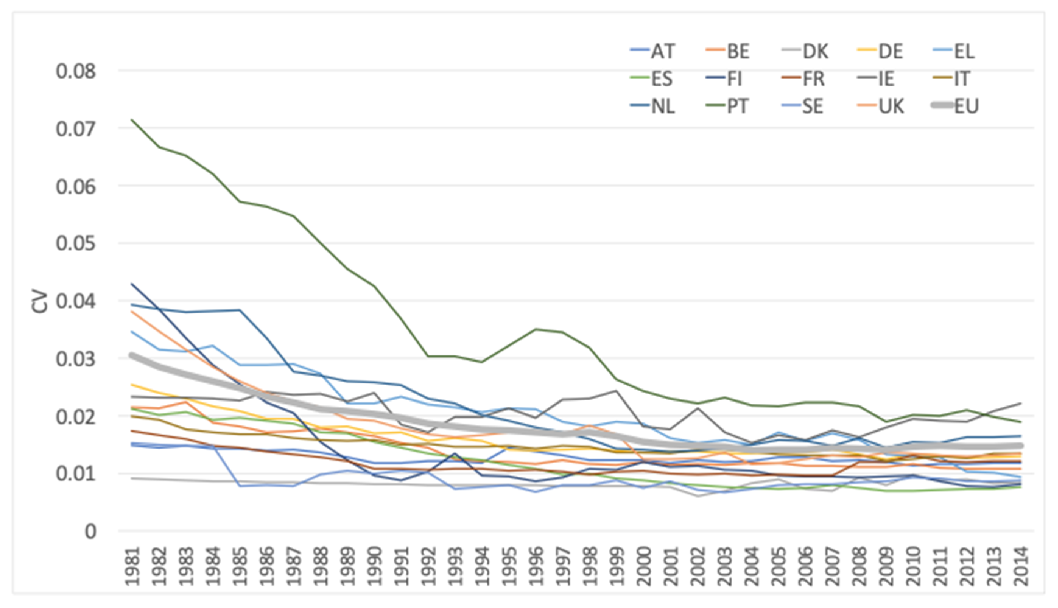
Reducing regional disparities is one of the main objectives of the European Cohesion Policy. The evolution of regional disparities, in the long run, of EU regions can be evaluated through the $\sigma$-convergence approach. In our analysis, to estimate $\sigma$-convergence, we use the coefficient of variation ($CV$) of logarithms of GDP per worker in Purchasing Power Standards (PPS, see Equation (1)). The $\sigma$-convergence analysis is carried out on NUTS 3 EU regions for the period 1981–2014.

If there is a declining long-term trend of $CV$, then there is a reduction of regional disparities and the σ-convergence is verified.

Figure 1 presents the coefficient of variation of the logarithms of GDP per worker in PPS computed considering EU NUTS 3 regions as a whole and for the 14 EU countries available between 1981–2014. Luxembourg is not included in the analysis, having only one NUTS 3 region.

As depicted in Figure 1, the coefficient of variation of the logarithms of GDP per worker in PPS for EU NUTS 3 regions as a whole (bold grey line) generally decreases from 1981 to 2014, falling from about 3% to 1.5%. The declining trend is stronger from 1981–1994, but the disparities slightly increased in 1995, and remained stable up to 1998. The disparities continued to decrease in 1999 and remained relatively stable up to the end of the period under investigation. These results reveal that $\sigma$-convergence happened within the EU NUTS 3 regions only for the first period (i.e., 1981–1999). These results are consistent with the empirical findings of previous analyses [1,48,49,50].

The falling of the hypothesis of $\sigma$-convergence among the EU regions does not exclude the possibility of different trends in each considered country (i.e., analysis of the within-country $\sigma$-convergence process). Strong evidence of $\sigma$-convergence from 1980 to the beginning of the 1990s is reported for some countries, such as Finland, the Netherlands, and Portugal. Conversely, Denmark shows a stable path of $CV$ (at a lower level) across the whole period under investigation.

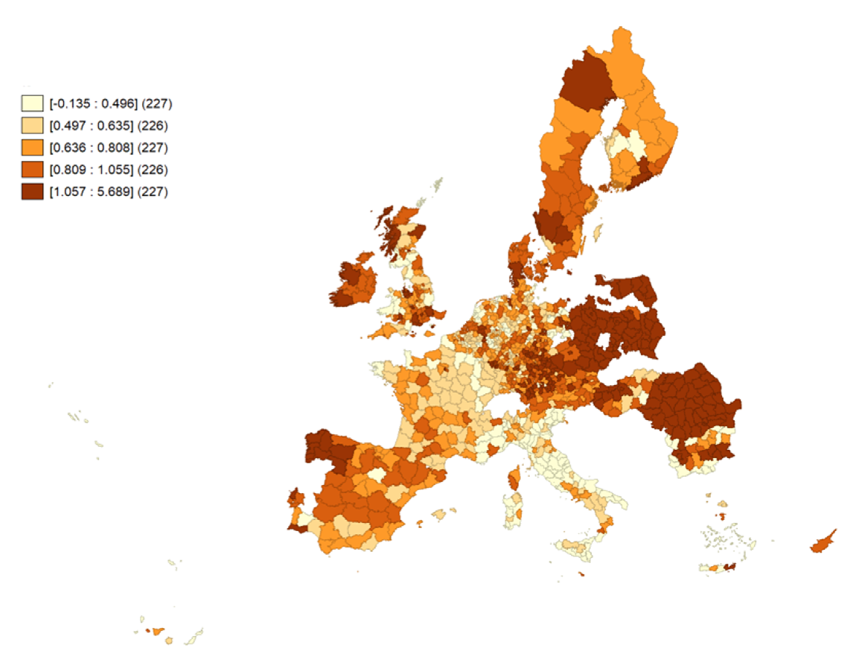
However, an important step of a territorial analysis concerns the investigation of the importance of spatial effects on the geographical distribution of the main variable for measuring economic growth. To this end, we decide to explore the spatial patterns of growth rates of GDP per worker in PPS, focusing the analysis only on the sample constituted by 1133 NUTS 3 regions across the period 1991–2014.

In Figure 2, we present the quantile maps of the growth rates of GDP per worker in PPS. Darker colours indicate the regions with higher values of the GDP per worker growth rates, while light colours refer to lower values of the GDP per worker growth rate. Higher growth rates are related to some regions in Northern Europe and some regions in Northern Spain. A certain dualism between Eastern and Western Europe is also observed, as high growth rates are reported for a large number of regions from Poland, Romania, and (formerly) East Germany. Conversely, France and Italy return lower economic growth rates. Additionally, regions of Spain and Ireland experienced higher growth in the whole period with few exceptions.

From the analysis of the geography of economic growth reported in Figure 1, it is evident the presence of relationships between neighbors (i.e., spatial dependence).

Table 1. Moran’s I statistics for the annual growth rate of GDP per worker in PPS. Connectivity matrix based on $K=7$ nearest neighbors.

Year	Moran’s I	Expectation	Standard Deviation	p−Value
1992	0.543	−0.001	0.0002	0.000
1993	0.420	−0.001	0.0002	0.000
1994	0.437	−0.001	0.0002	0.000
1995	0.163	−0.001	0.0002	0.000
1996	0.273	−0.001	0.0002	0.000
1997	0.264	−0.001	0.0002	0.000
1998	0.183	−0.001	0.0002	0.000
1999	0.243	−0.001	0.0003	0.000
2000	0.211	−0.001	0.0002	0.000
2001	0.286	−0.001	0.0002	0.000
2002	0.396	−0.001	0.0002	0.000
2003	0.241	−0.001	0.0002	0.000
2004	0.398	−0.001	0.0002	0.000
2005	0.080	−0.001	0.0002	0.000
2006	0.310	−0.001	0.0002	0.000
2007	0.246	−0.001	0.0002	0.000
2008	0.315	−0.001	0.0002	0.000
2009	0.237	−0.001	0.0002	0.000
2010	0.267	−0.001	0.0002	0.000
2011	0.260	−0.001	0.0002	0.000
2012	0.274	−0.001	0.0002	0.000
2013	0.268	−0.001	0.0002	0.000
2014	0.394	−0.001	0.0002	0.000

displays the Moran’s $I$ index, for evaluating spatial dependence, computed for each year from 1992–2014. The index is calculated for the annual growth rates of GDP per worker in PPS. In the computation of the Moran’s $I$, we consider a row-standardised contiguity matrix, based on the $K$ nearest neighbors’ criterion with $K=7$. All statistics have values larger than the expected value and are highly significant. The inference is based on a random permutation approach with 10,000 permutations. The results indicate the presence of positive spatial autocorrelation, and thus, that regions with similar values of the GDP per worker growth rate tend to cluster together in space.

This result corroborates the idea that spatial information cannot be neglected in the analysis of regional economic convergence. As described in the introduction, economic convergence represents a basic measure for the evaluation of the effectiveness of the EU Cohesion Policy. The $\beta$-convergence analysis sheds light on the catch-up process, in terms of GDP per worker growth, between economies consequently producing a reduction of regional disparities. In this section, we describe the main results of the empirical analysis focused on conditional $\beta$-convergence for EU NUTS 3 regions. In particular, we estimate the spatially augmented Solow model defined in Equation (4).

The dependent variable, $g$, conveys the average growth rate of GDP per worker in PPS over the period under investigation. The variable $v$ is expressed as $v=n+l+k$, where $n$ is the working population growth rate, and $l+ k=0.05$ [21]. The fraction of output invested in physical capital, $s^k$, is defined as the average, over the period under investigation, of the investments expressed as a share of GDP.

Data on investment not available at NUTS 3 level can be derived by applying the BIM described in Section 4.1. This procedure allows the disaggregation of data on investment of physical capital (i.e., gross fixed capital formation) that are available at a more aggregate geographical level (i.e., for NUTS 2 regions). A correspondence between aggregated and disaggregated data is established by the matrix $P,$ which is defined as an $M\times N$ matrix, with $M$ as the number of NUTS 2 regions and$N$ as the number of NUTS 3 units. The elements of the matrix $P$ are such that $p_{ij}=1$ if the $jth$ NUTS 3 unit belongs to the $ith$ NUTS 2 region, and $p_{ij}=0$ otherwise. Hence, the aggregation proceeds through a sum operation. In the covariance structure of the process, the proximity matrix $W$ is specified according to the $K$ nearest neighbors’ criterion, with $K=7$, and the extent of the spatial autocorrelation parameter, $\rho$, is defined according to the spatial dependence observed at the NUTS 2 level.

Table 2. Estimation results for alternative models for $\beta$ -convergence analysis (1981–2014), using cross-sectional data, 901 NUTS 3 European regions.

	Non-Spatial Absolute Model	Non-Spatial Conditional Model	Weights Matrix: 7 Nearest Neighbors
			SDM Conditional Model ML	SDM Conditional Model GS2SLS-Het.
	Coefficient (standard error)	Coefficient (standard error)	Coefficient (standard error)	Coefficient (standard error)
Constant	0.2633 *** (0.0048)	0.2856 *** (0.0071)	0.0948 *** (0.0126)	0.0191 (0.0443)
$\ln y_{1981}$	−0.0232 *** (0.0005)	−0.0239 *** (0.0005)	−0.0269 *** (0.0005)	−0.0271 *** (0.0009)
$\ln s^k$		0.0000 (0.0000)	0.0001 ** (0.0000)	0.0001 * (0.0000)
$\ln v=\ln \left(n+l+k\right)$		0.0053 *** (0.0012)	0.0056 *** (0.0012)	0.0058 *** (0.0016)
$W\ln y_{1981}$			0.0194 *** (0.0011)	0.0257 *** (0.0038)
$W \ln s^k$			−0.0001 (0.0001)	−0.0001 (0.0001)
$W \ln v$			−0.0032 * (0.0020)	−0.0049 * (0.0025)
$\rho$			0.5973 *** (0.0361)	0.9067 *** (0.1781)
$\lambda$ (Convergence Rate)	4.57%	4.93%	7.24%	7.48%
Moran’s Test		0.3291 ***
Breusch-Pagan		46.14 ***
Studentized Breusch-Pagan		23.77 ***
$AIC$	−7212.03	−7226.67	−7493.94
$R^2$	0.7158	0.7216	0.7485	0.7447

Significance levels: *** 1%, ** 5%, * 10%.

presents the results from alternative models estimated on data from ARDECO dataset for the period 1981–2014.

For the non-spatial specifications (see column 1 and 2 of Table 2), we estimate a speed of convergence higher than the usual of about 2% [22]. These results are coherent with empirical findings of some other analysis carried out for EU regions [10,51].

For the non-spatial conditional model (see column 2 of Table 2), the Moran’s test for spatial autocorrelation is positive and highly significant, highlighting the presence of spatial dependence.

In the SDM specification defined in Equation (4), the spatially lagged dependent variable as well as the spatial lags of the independent variables are included as explanatory variables. In this specification, we use a contiguity matrix based on the$K=7$ nearest neighbor criterion. We tested different specifications of the proximity matrix, based on different numbers of neighbors. We selected $K=7$ corresponding to the lower value of the $AIC$, and thus to the better fit of the model. Moreover, this choice is consistent with the idea of avoiding the presence of non-connected regions (for similar considerations related to NUTS 2 regions, see [27]).

The SDM model is estimated by using the ML method, using STATA software, and is presented in column 3 of Table 2. However, the Breusch–Pagan test reveals the presence of heteroscedasticity that, for geographically distributed data, appears reasonable, since the observational units are likely to be characterized by different sizes and differences in other structural features [10,44]. For this reason, we employ the GS2SLS estimator corrected for the presence of heteroscedasticity described in Section 4.2 (see column 4 of Table 2).

For all the models, the estimation confirms the convergence process (i.e., $\beta <0$ and significant), and the coefficients have the predicted signs, with the exception of the coefficients associated to the variable $v$ and its spatial lag. Generally, parameter estimates are highly significant. Positive and significant estimates are found for the spatial autocorrelation parameters $\rho$. The values of $AIC$ and $R^2$ show the better fit of spatial models with respect to the non-spatial specifications.

As displayed in Table 2, the rate of convergence tends to be higher when the spatial dependence is considered (see columns 3 and 4 of Table 2). Finally, note that the estimates of the SDM obtained with ML and GS2SLS -Het. methods are very similar in the magnitude of the coefficient and their significance.

In

Table 3. Average direct, indirect, and total impacts of the explanatory variables (1981–2014) for the spatial heteroscedastic model estimated with GS2SLS, 901 NUTS 3 European regions.

Model	Variable	Average Direct Impact	Average Indirect Impact	Average Total Impact
Conditional model with heterosc. GS2SLS	$\ln y_{1981}$	−0.0266 *** (0.0010)	0.0124 (0.0131)	−0.0142 (0.0134)
	$\ln s^k$	0.0001 (0.0001)	0.0002 (0.0008)	0.0003 (0.0008)
	$\ln v$	0.0060 *** (0.0018)	0.0039 (0.0194)	0.0099 (0.0202)

Significance levels: *** 1%, ** 5%, * 10%.

, results on the average impacts of the spatial heteroscedastic model are reported. Significant average direct impacts are reported for the initial level of GDP per worker and for the variable $v$. The average direct impact estimate associated with $\ln y_{1981}$ indicates that a 1% increase in the initial level of GDP per worker registered by a specific region is associated with a decrease in its subsequent growth rate of −0.0266%.

For the period 1991–2014, the group of regions under investigation is enlarged to include the regions belonging to Eastern Europe.

Table 4. Estimation results for alternative models for $\beta$ -onvergence analysis (1991–2014), using cross-sectional data, 1133 NUTS 3 European regions.

	Non-Spatial Absolute Model	Non-Spatial Conditional Model	Weights Matrix: 7 Nearest Neighbors
			SDM Conditional Model	Conditional Model with Heterosc. GS2SLS
	Coefficient (standard error)	Coefficient (standard error)	Coefficient (standard error)	Coefficient (standard error)
Constant	0.2238 *** (0.0047)	0.2350 *** (0.0077)	0.1044 *** (0.0129)	0.0172 (0.0523)
$\ln y_{1991}$	−0.0193 *** (0.0005)	−0.0199 *** (0.0006)	−0.0216 *** (0.0009)	−0.0211 *** (0.0017)
$\ln s^k$		−0.0001 (0.0001)	0.0000 (0.0000)	0.0000 (0.0000)
$\ln v=\ln \left(n+l+k\right)$		0.0019 * (0.0010)	−0.0021 ** (0.0009)	−0.0027 ** (0.0013)
$W\ln y_{1991}$			0.0135 *** (0.0013)	0.0198 *** (0.0042)
$W \ln s^k$			−0.0001 * (0.0001)	−0.0001 (0.0001)
$W \ln v$			0.0072 *** (0.0016)	0.0037 (0.0029)
$\rho$			0.6527 *** (0.0297)	0.9473 *** (0.1617)
$\lambda$ (Convergence Rate)	2.60%	2.71%	3.04%	2.94%
Moran’s $I$		0.3946 ***
Breusch-Pagan		373.45 ***
Studentized Breusch-Pagan		103.70 ***
$AIC$	−7973.93	−7974.20	−8378.15
$R^2$	0.6129	0.6143	0.6484	0.6517

Significance levels: *** 1%, ** 5%, * 10%.

displays the estimation results for the non-spatial and the spatial specifications for this new sample. Also in this case, the Moran’s test on the OLS residuals highlights the presence of spatial dependence and the need for the use of a spatial augmented approach. The significance of Breusch–Pagan’s test of heteroscedasticity corroborates the choice of using the GS2SLS-Het. estimator.

Table 5. Average direct, indirect, and total impacts of the explanatory variables (1991–2014) for the spatial heteroscedastic model estimated with GS2SLS, 1133 NUTS 3 European regions.

Model	Variable	Average Direct Impact	Average Indirect Impact	Average Total Impact
Conditional model with heterosc. GS2SLS	$\ln y_{1991}$	−0.0212 *** (0.0017)	−0.0038 (0.0142)	−0.0250 * (0.0143)
	$\ln s^k$	−0.0001 (0.0001)	−0.0005 (0.0014)	−0.0006 (0.0015)
	$\ln v$	−0.0020 (0.0019)	0.0206 (0.0363)	0.0186 (0.0372)

Significance levels: *** 1%, * 10%.

shows the estimated direct, indirect, and total impacts for the variables of the heteroscedastic model for 1133 NUTS 3 European regions of this second sample. For the initial level of GDP per worker, we found a negative and significant total effect. This reveals that a 1% increase in the initial level of GDP per worker determines a decrease of −0.0212% on the GDP per worker growth rate. Furthermore, the average direct impact associated with this variable is negative and significant.

Globally, the different analyses performed in this section ensure the presence of a convergence process for the EU NUTS 3 regions.

Our results confirm that convergence tends to be faster when spatial interaction effects are accounted for. This result is consistent with some previous literature that, based on cross-sectional analyses, shows an increase in the estimated speed of convergence in the presence of spatial effects (see, among others [10,52]). This indicates that omitting the spatial interaction effects would lead to a biased estimation of the convergence rate. Moreover, adopting a panel data approach may cause difficulties in comparing to others cross sectional studies in terms of speed of convergence [14].

6. Discussion

The persistence of regional disparities across EU regions has intensified since the years that preceded the global crisis of 2008. As pointed out by the study of $\sigma$-convergence, after progressive years of reduction of regional disparities, this phenomenon seems to have stopped due to economic and financial circumstances that affect the European Union. Hence, those circumstances call for a deeper look at the dynamics that regulate regional economic convergence to ensure regional equity both within and across countries.

As pointed out by [12], regional disparities become more evident when considering smaller territorial units, and policies aimed at reducing disparities should be targeted to a more detailed spatial scale, consistently with a place-sensitive approach [5]. In fact, the achievement of fairness requires the reduction of local disparities, specifically income and living standards, as well as the promotion of social inclusion and opportunities of employment. Undoubtedly, regional economic convergence has been extensively studied since the 1990s to this end [6]. Despite that, two major issues remain open.

On the one hand, the spatial scale represented a constraint for many analyses of regional economic convergence in the EU [53]. Analyses at NUTS 2 level have revealed their importance in terms of support to the European regional policies [54]. However, the progressive data availability and the use of spatial disaggregation tools allow for more refined analyses, enabling us to target very local issues, including spatial interdependencies between local communities.

On the other hand, the need for analyses that take into account spatial features is more relevant due to the increasing interconnections that occur at the regional level between EU regions. Those interconnections reveal that regional economies are nested and that empirical attempts to verify reduction in disparities cannot discard interdependencies. Our results stress changes between spatial and non-spatial specifications in the outputs of the growth function. However, paying further attention to the spatial dimension is not merely concerned to technical aspects, but it can lead to more accurate evidence of spillover effects.

From a policy perspective, the results highlight differences in the convergence speed between the spatial and non-spatial model. This aspect may be of extreme importance to policy makers as it leads to an additional component to take into account to reduce disparities between regions. In fact, our analyses verify the global presence of convergence as for previous analyses involving the European Union (see, among others, [52,55]). However, positive local spillovers may not have any suitable effect when low growth levels are present in the neighbours.

Further, the results from the analysis of two different time periods are also interesting. In fact, the first group (1981–2104) includes traditionally open and liberal economies, while the second group (1991–2014) combines regions from both Western and Eastern regions. When the analysis considers both Western and Eastern European regions, we note lower speed of convergence, that slightly rises with the introduction of spatial effects in the model. This result is emphasized as the convergence is faster between more similar regions, mainly confirming empirical findings in some previous literature. As pointed out by [12], the speed of convergence is slowing down in the European Union, and our evidence seems to confirm that part of this slowing issue may be caused by the substantial heterogeneity that was introduced by the entrance of Eastern regions. Similarly, [56] highlighted that the slowing down of the convergence rate between EU regional economies could be interpreted as the result of a variety of factors, among which are the lower growth rates induced by periods of economic crises as well as the effect of the EU integration process. The strong disparities existing between EU regions in terms of initial resources endowment and subsequent growth performances thus affect their ability to converge towards the same steady state. This result appears to support the idea that additional attention should be paid to regions from Eastern Europe in order to ensure cohesion and confirm the relevance of regional policies aimed at reducing regional disparities. In this direction, a progressive integration of Eastern European economies could produce positive results in a more homogenous growth path, also thanks to the presence of spillovers. From this perspective, promoting the reduction of inequalities and triggering economic convergence among regions could represent not only a solution to an economic problem, but also a necessary condition for achieving social and political stability for the EU and its member states [5].

7. Concluding Remarks

In this paper, we highlight the importance of spatial information in the analysis of regional economic $\beta$-convergence. The analyses performed on a refined spatial scale at NUTS 3 give us a more detailed picture on the existence of a conditional $\beta$-convergence process. NUTS 3 regions are considered in order to extend a wide body of literature that analyses European convergence at the NUTS 2 level and to go more “local” to support specific policies. This geographical scale of analysis poses some issues, mainly related to the presence of missing observations for some variables of interest. Given the availability of data at a coarse geographical level, we estimated these missing observations by applying an areal interpolation procedure that accounts for the spatial nature of data. This allowed to assess the convergence process at the sub-regional level.

The convergence process is here interpreted in terms of a reduction of disparities experienced by regional economies. Different analyses were performed to measure the presence of economic convergence according to the period of investigation, regions considered, and used techniques.

Our results verify that an augmented theoretical model of growth that considers spatial interdependencies is appropriate for the analysis of EU regional economic convergence. The evidence shows that the growth rate of GDP per worker in a region is not only a function of traditional determinants as investment and population growth, but also that the spillover must be quantified and considered for analysis and policy definition.

The main results confirm that regional economic $\beta$-convergence holds at the European level across the different periods and regions investigated.

Finally, the present paper highlights the need for major integration between Western and Eastern European regions in order to support cohesion and reduce disparities in the whole EU.

References

- Monfort, P. Convergence of EU regions: Measures and evolution. European Commission. Reg. Policy 2008, 1, 1–20. [Google Scholar]
- Artelaris, P.; Petrakos, G. Intraregional Spatial Inequalities and Regional Income Level in the EU: Beyond the Inverted-U hypothesis. Int. Reg. Sci. Rev. 2016, 39, 291–317. [Google Scholar] [CrossRef]
- Capello, R.; Perucca, G. Understanding citizen perception of European Union Cohesion Policy: The role of the local context. Reg. Stud. 2018, 52, 1451–1463. [Google Scholar] [CrossRef] [Green Version]
- Ezcurra, R.; Rios, V. Quality of government and regional resilience in the European Union. Evidence from the Great Recession. Pap. Reg. Sci. 2019, 98, 1267–1290. [Google Scholar] [CrossRef]
- Iammarino, S.; Rodríguez-Pose, A.; Storper, M. Regional inequality in Europe: Evidence, theory and policy implications. J. Econ. Geogr. 2019, 19, 273–298. [Google Scholar] [CrossRef]
- Barro, R.J.; Sala-i-Martin, X. Economic Growth Theory; Mc Graw-Hill: Boston, MA, USA, 1995. [Google Scholar]
- Postiglione, P.; Andreano, M.S.; Benedetti, R. Using constrained optimization for the identification of convergence clubs. Comput. Econ. 2013, 42, 151–174. [Google Scholar] [CrossRef]
- Cartone, A.; Panzera, D.; Postiglione, P.; Viñuela, A. Deliverable 3.2. Report on Economic Growth in EU Territories, IMAJINE WP3 Territorial Inequalities and Economic Growth. 2019.
- Geppert, K.; Stephan, A. Regional disparities in the European Union: Convergence and agglomeration. Pap. Reg. Sci. 2008, 87, 193–217. [Google Scholar] [CrossRef] [Green Version]
- Panzera, D.; Postiglione, P. Economic growth in Italian NUTS 3 provinces. Ann. Reg. Sci. 2014, 53, 273–293. [Google Scholar] [CrossRef]
- Goecke, H.; Hüther, M. Regional convergence in Europe. Intereconomics 2016, 51, 165–171. [Google Scholar] [CrossRef] [Green Version]
- Butkus, M.; Cibulskiene, D.; Maciulyte-Sniukiene, A.; Matuzeviciute, K. What is the evolution of convergence in the EU? Decomposing EU disparities up to the NUTS 3 level. Sustainability 2018, 10, 1552. [Google Scholar] [CrossRef] [Green Version]
- Islam, N. Growth empirics: A panel data approach. Q. J. Econ. 1995, 110, 1127–1170. [Google Scholar] [CrossRef]
- Elhorst, J.P.; Piras, G.; Arbia, G. Growth and convergence in a multi-regional model with space-time dynamics. Geogr. Anal. 2010, 42, 338–355. [Google Scholar] [CrossRef]
- Abreu, M.; De Groot, H.L.F.; Florax, R.J.G.M. A meta-analysis of β-convergence: The legendary 2%. J. Econ. Surv. 2005, 19, 389–420. [Google Scholar] [CrossRef]
- Arbia, G.; Le Gallo, J.; Piras, G. Does evidence on regional economic convergence depend on the estimation strategy? Outcomes from analysis of a set of NUTS2 EU regions. Spat. Econ. Anal. 2008, 3, 209–224. [Google Scholar] [CrossRef]
- Solow, R.M. A contribution to the theory of economic growth. Q. J. Econ. 1956, 70, 65–94. [Google Scholar] [CrossRef]
- Barro, R.J.; Sala-i-Martin, X. Convergence. J. Political Econ. 1992, 100, 223–251. [Google Scholar] [CrossRef]
- Islam, N. What have we learnt from the convergence debate? J. Econ. Surv. 2003, 17, 311–361. [Google Scholar] [CrossRef] [Green Version]
- Gluschenko, K. Measuring regional inequality: To weight or not to weight? Spat. Econ. Anal. 2018, 13, 36–59. [Google Scholar] [CrossRef]
- Mankiw, N.G.; Romer, D.; Weil, D.N. A contribution to the empirics of economic growth. Q. J. Econ. 1992, 107, 407–437. [Google Scholar] [CrossRef]
- Sala-i-Martin, X. The classical approach to convergence analysis. Econ. J. 1996, 106, 1019–1036. [Google Scholar] [CrossRef]
- Rey, S.J.; Montouri, B.D. US regional income convergence: A spatial econometric perspective. Reg. Stud. 1999, 33, 143–156. [Google Scholar] [CrossRef]
- Tobler, W.R. A computer movie simulating urban growth in the Detroit Region. Econ. Geogr. Suppl. 1970, 46, 234–240. [Google Scholar] [CrossRef]
- Anselin, L. Spatial Econometrics: Methods and Models; Academic Publishers: Dordrecht, The Netherlands, 1988. [Google Scholar]
- Lόpez-Bazo, E.; Vayá, E.; Mora, A.J.; Suriñach, J. Regional economic dynamics and convergence in the European Union. Ann. Reg. Sci. 1999, 3, 343–370. [Google Scholar]
- Le Gallo, J.; Ertur, C. Exploratory spatial data analysis of the distribution of regional per capita GDP in Europe, 1980–1995. Pap. Reg. Sci. 2003, 82, 175–201. [Google Scholar] [CrossRef] [Green Version]
- Ertur, C.; Koch, W. Growth, technological interdependence and spatial externalities: Theory and evidence. J. Appl. Econ. 2007, 22, 1033–1062. [Google Scholar] [CrossRef] [Green Version]
- LeSage, J.; Fischer, M.M. Spatial growth regressions: Model, specification, estimation and interpretation. Spat. Econ. Anal. 2008, 3, 275–304. [Google Scholar] [CrossRef] [Green Version]
- LeSage, J.P.; Pace, R.K. Introduction to Spatial Econometrics; Taylor & Francis: Boca Raton, FL, USA, 2009. [Google Scholar]
- Abreu, M.; De Groot, H.L.F.; Florax, R.J.G.M. Space and growth: A survey of empirical evidence and methods. Région Et Développement 2005, 21, 13–44. [Google Scholar] [CrossRef] [Green Version]
- Lilburne, L.; Tarantola, S. Sensitivity analysis of spatial models. Int. J. Geogr. Inf. Sci. 2009, 23, 151–168. [Google Scholar] [CrossRef] [Green Version]
- Taner, T. Optimisation processes of energy efficiency for a drying plant: A case of study for Turkey. Appl. Eng. 2015, 80, 247–260. [Google Scholar] [CrossRef]
- Taner, T.; Sivrioglu, M. Energy-exergy analysis and optimisation of a model sugar factory in Turkey. Energy 2015, 93, 641–654. [Google Scholar] [CrossRef]
- Taner, T. Energy and exergy analyze of PEM fuel cell: A case study of modeling and simulations. Energy 2018, 143, 284–294. [Google Scholar] [CrossRef]
- Panzera, D.; Benedetti, R.; Postiglione, P. A Bayesian approach to parameter estimation in the presence of spatial missing data. Spat. Econ. Anal. 2016, 11, 201–218. [Google Scholar] [CrossRef]
- Goodchild, M.F.; Lam, N.S. Areal interpolation: A variant of the traditional spatial problem. Geo-Processing 1980, 1, 297–312. [Google Scholar]
- Goodchild, M.F.; Anselin, L.; Deichmann, U. A framework for the areal interpolation of socioeconomic data. Environ. Plann. A 1993, 25, 383–397. [Google Scholar] [CrossRef]
- Murakami, D.; Tsutsumi, M. Practical spatial statistics for areal interpolation. Environ. Plann. B 2012, 39, 1016–1033. [Google Scholar] [CrossRef]
- Benedetti, R.; Palma, D. Markov random field-based image subsampling method. J. Appl. Stat. 1994, 21, 495–509. [Google Scholar] [CrossRef]
- Besag, J. Spatial interaction and the statistical analysis of lattice systems. J. R. Stat. Soc. B 1974, 36, 192–225. [Google Scholar] [CrossRef]
- Tobler, W.R. Smooth pycnophylactic interpolation for geographical regions. J. Am. Stat. Assoc. 1979, 74, 519–530. [Google Scholar] [CrossRef]
- Rey, S.J.; Le Gallo, J. Spatial analysis of economic convergence. In Palgrave Handbook of Econometrics; Mills, T.C., Patterson, K., Eds.; Palgrave Macmillan: London, UK, 2009; pp. 1251–1290. [Google Scholar]
- Piras, G.; Postiglione, P.; Aroca, P. Specialization, R&D and productivity growth: Evidence from EU regions. Ann. Reg. Sci. 2012, 49, 35–51. [Google Scholar]
- Kelejian, H.H.; Prucha, I.R. Specification and estimation of spatial autoregressive models with autoregressive and heteroskedastic disturbances. J. Econ. 2010, 157, 53–67. [Google Scholar] [CrossRef] [Green Version]
- Arraiz, I.; Drukker, D.M.; Kelejian, H.H.; Prucha, I.R. A spatial Cliff–Ord-type model with heteroskedastic innovations: Small and large sample results. J. Reg. Sci. 2010, 50, 592–614. [Google Scholar] [CrossRef] [Green Version]
- Drukker, D.M.; Egger, P.H.; Prucha, I.R. On two-step estimation of a spatial autoregressive model with autoregressive disturbances and endogenous regressors. Econ. Rev. 2013, 32, 686–733. [Google Scholar] [CrossRef]
- Neven, D.; Gouyette, C. Regional convergence in the European Union. J. Common Mark. Stud. 1995, 33, 47–65. [Google Scholar] [CrossRef]
- Ertur, C.; Le Gallo, J.; Baumont, C. The European regional convergence process, 1980–1995: Do spatial regimes and spatial dependence matter? Int. Reg. Sci. Rev. 2006, 29, 3–34. [Google Scholar] [CrossRef]
- Monfort, P. The role of international transfers in public investment in CESEE: The European Commission’s experience with Structural Funds. Eur. Comm. Reg. Policy 2012, 2, 1–12. [Google Scholar]
- Fischer, M.M.; Stirböck, C. Pan-European regional income growth and club-convergence. Ann. Reg. Sci. 2006, 40, 693–721. [Google Scholar] [CrossRef] [Green Version]
- Ramajo, J.; Marquez, M.A.; Hewings, G.J.; Salinas, M.M. Spatial heterogeneity and interregional spillovers in the European Union: Do cohesion policies encourage convergence across regions? Eur. Econ. Rev. 2008, 52, 551–567. [Google Scholar] [CrossRef]
- Rey, S.J.; Janikas, M.V. Regional convergence, inequality, and space. J. Econ. Geog. 2005, 5, 155–176. [Google Scholar] [CrossRef]
- Dall’erba, S.; Le Gallo, J. Regional convergence and the impact of European structural funds over 1989–1999: A spatial econometric analysis. Pap. Reg. Sci. 2008, 87, 219–244. [Google Scholar] [CrossRef] [Green Version]
- Andreano, M.S.; Benedetti, R.; Postiglione, P. Spatial regimes in regional European growth: An iterated spatially weighted regression approach. Qual. Quant. 2017, 51, 2665–2684. [Google Scholar] [CrossRef]
- Cuadrado-Roura, J.R. Regional convergence in the European Union: From hypothesis to the actual trends. Ann. Reg. Sci. 2001, 35, 333–356. [Google Scholar] [CrossRef]
Figure 1.
-convergence analysis—coefficient of variation (CV) of , NUTS 3 regions.
Figure 2.
Quantile map of GDP per worker growth rate from 1991–2014.