Hydroclimatic Effects of a Hydropower Reservoir in a Tropical Hydrological Basin


1
Civil and Agricultural Engineering Department, Water Resources Research Group (GIREH), Universidad Nacional de Colombia, Bogotá 111321, Colombia
2
Instituto de Estudios Ambientales, Universidad Nacional de Colombia, Bogotá 111321, Colombia
3
Department of Physical Geography, Stockholm University, 10691 Stockholm, Sweden
4
Baltic Sea Centre, Stockholm University, 10691 Stockholm, Sweden
*
Authors to whom correspondence should be addressed.
Sustainability 2020, 12(17), 6795; https://0-doi-org.brum.beds.ac.uk/10.3390/su12176795
Submission received: 13 July 2020
/
Revised: 15 August 2020
/
Accepted: 18 August 2020
/
Published: 21 August 2020
(This article belongs to the Special Issue Watershed Modelling and Management for Sustainability)
Abstract
:The consequent change in land cover from vegetation to water surface after inundation is the most obvious impact attributed to the impoundment of reservoirs and dam construction. However, river regulation also alters the magnitude and variability of water and energy fluxes and local climatic parameters. Studies in Mediterranean, temperate and boreal hydrological basins, and even a global-scale study, have found a simultaneous decrease in the variation of runoff and increase in the mean evaporative ratio after impoundment. The aim here is to study the existence of these effects on a regulated tropical basin in Colombia with long-term data, as such studies in tropical regions are scarce. As expected, we observed a decrease in the long-term coefficient of variation of runoff of 33% that can be attributed to the impoundment of the reservoir. However, we did not find important changes in precipitation or the expected increasing evaporative ratio-effect from the impoundment of the reservoir, founding for the latter rather a decrease. This may be due to the humid conditions of the region where actual evapotranspiration is already close to its potential or to other land cover changes that decrease evapotranspiration during the studied period. Our study shows that the effects from impounded reservoirs in tropical regulated basins may differ from those found in other climatic regions.
1. Introduction
The water cycle is not only a generator of ecosystem services and a critical agent of change in the Earth system; it is also a system that is subject to intense human interference. The resilience of water systems regulates the state of the ecosystems and biomes through interaction and feedback of the ecological functions related to water [1]. Out of the many important factors, climate variability and changes in land use/land cover (LULC) appear to be the main drivers of changes in these functions and in the availability of fresh water on land [2]. The storage and redistribution of water for agriculture and energy production, by irrigation and impoundment of water in artificial reservoirs is also known to induce important changes in the availability and variability of water [3,4,5,6] by increasing evaporation from the artificial reservoirs and regulating the flow of water [7,8,9]. These effects induce significant physical and ecological impacts on dependent terrestrial and aquatic ecosystems [10,11]. The effects of reservoirs have also been identified in variables of the hydrological cycle other than runoff (R). For example, Degu et al. [12] found that the presence of large reservoirs increases the extreme daily precipitation (P) (on 50th, 90th, 95th, and 99th percentiles) in the vicinity of the reservoirs in Mediterranean and arid climates. Hossain [13] found an increase in extreme precipitation after the filling of the reservoirs in southern Africa, India, the western United States, and Central Asia. On the other hand, Zhao et al. [14] found no important changes in monthly precipitation before and after the construction of a dam in humid-subtropical China.
Another hydrological variable affected by the impoundment of reservoirs is evapotranspiration, which is very important from local to global scales, as it regulates the energetic balance of the Earth and the climate system through carbon sequestration and water transport [15,16,17]. Destouni et al. [18] found that the development of hydroelectric projects in Sweden simultaneously increased the evaporative ratio in the hydrological basins where the projects were located and reduced the coefficient of variation of runoff downstream (CVR). The evaporative ratio is the actual evapotranspiration (AET) divided by precipitation (P) (i.e., AET/P). The global study of Jaramillo and Destouni [4] also found long-term net increases in AET/P in basins with intensive flow regulation and/or irrigation. Similar results were found by Levi et al. [19] in the transnational basin of the Sava River in Eastern Europe and by Wang and Hejazi [20] in the United States.
However, the number of studies on hydroclimatic evolution has focused in highly regulated basins (i.e., more than one large reservoir) and located mainly in regions that are not tropical. Evapotranspiration (ET) is one of the most important variables of the water budget. This variable affects the atmospheric content of water and it controls precipitation, including its influence on the absorption and reflection of solar and terrestrial radiation [21]. In the tropical context, it becomes a a challenge to separate the signatures of natural precipitation variability in the landscape from the LULC-induced and climate-induced changes on ET. The simultaneity of these impacts increases the importance to establish the origin of induced changes and to understand ecohydrological and climatic synergies on a basin scale.
Since changes in the hydrological cycle, resulting from water impoundment, will continue to condition the future responses of river systems and their functions and related ecosystem services [22], it is important to understand these historical changes and their drivers to establish adaptation measures and strategies for the management of water resources.
The main aim of this study is to identify the effects of hydropower, if any, on hydroclimatic variables such as precipitation, runoff and evapotranspiration in a tropical basin in Colombia with good data availability and that has been regulated by a single impounded reservoir. Most of the results of these type of studies have been done in Mediterranean, temperate and boreal catchments, with a lack of scientific literature on the hydroclimatic effects of impounded reservoirs in tropical regions.
Our initial hypothesis is that, in accordance with the other research studying the effects of impounded reservoirs mentioned above, tropical regulated basins such as the one studied here will show similar patterns of change as the ones observed in more temperate and boreal basins. These changes include: (1) a decrease in the coefficient of variation of runoff downstream, (2) an increase in the ratio of actual evapotranspiration to precipitation, and (3) possible change in the long-term magnitude of monthly precipitation in the vicinity of the reservoir. For this task, we aim to separate the effects from climate drivers from those of the impounded reservoir on evapotranspiration and runoff by combining statistical methods of change detection and effect-separation techniques. We searched for evidence of the long-term effects of a hydroelectric project on the hydroclimatic variables P, R and AET. The study was carried out at both monthly and annual scales and during the period between 1954 and 2014, according to runoff and precipitation data availability, in one of the most iconic regulated basins in Colombia, the Prado River basin.
2. Materials and Methods
2.1. Site and Hydroelectric Project Description
Colombia is a country highly dependent on water resources for energy production. Currently, there are 28 hydroelectric projects (net effective capacity (NEC) ≥ 20 MW) and 115 (NEC < 20 MW) projects totaling an installed volume capacity of 59 km3 of impounded water and a related installed hydroelectric generating capacity of 12.0 GW [23,24]. According to the Colombian Mining and Energy Planning Unit, the energetic demand of the country is projected to increase between 105 to 147% for the year 2050 in relation to that of 2010 [25]. Furthermore, 125 hydropower projects are in the pre-feasibility stage, that would add about 5600 MW to the existing installed capacity [26]. Since the hydroclimatic impacts of flow regulation from hydropower in Colombia and the corresponding effects on the climate, aquatic and terrestrial ecosystems have not been studied up to date, judging from the minimum amount of scientific publications in peer-reviewed journals, the construction of all these hydroelectric projects raises concern among environmental authorities, the communities in the areas of influence of such projects and its owners.
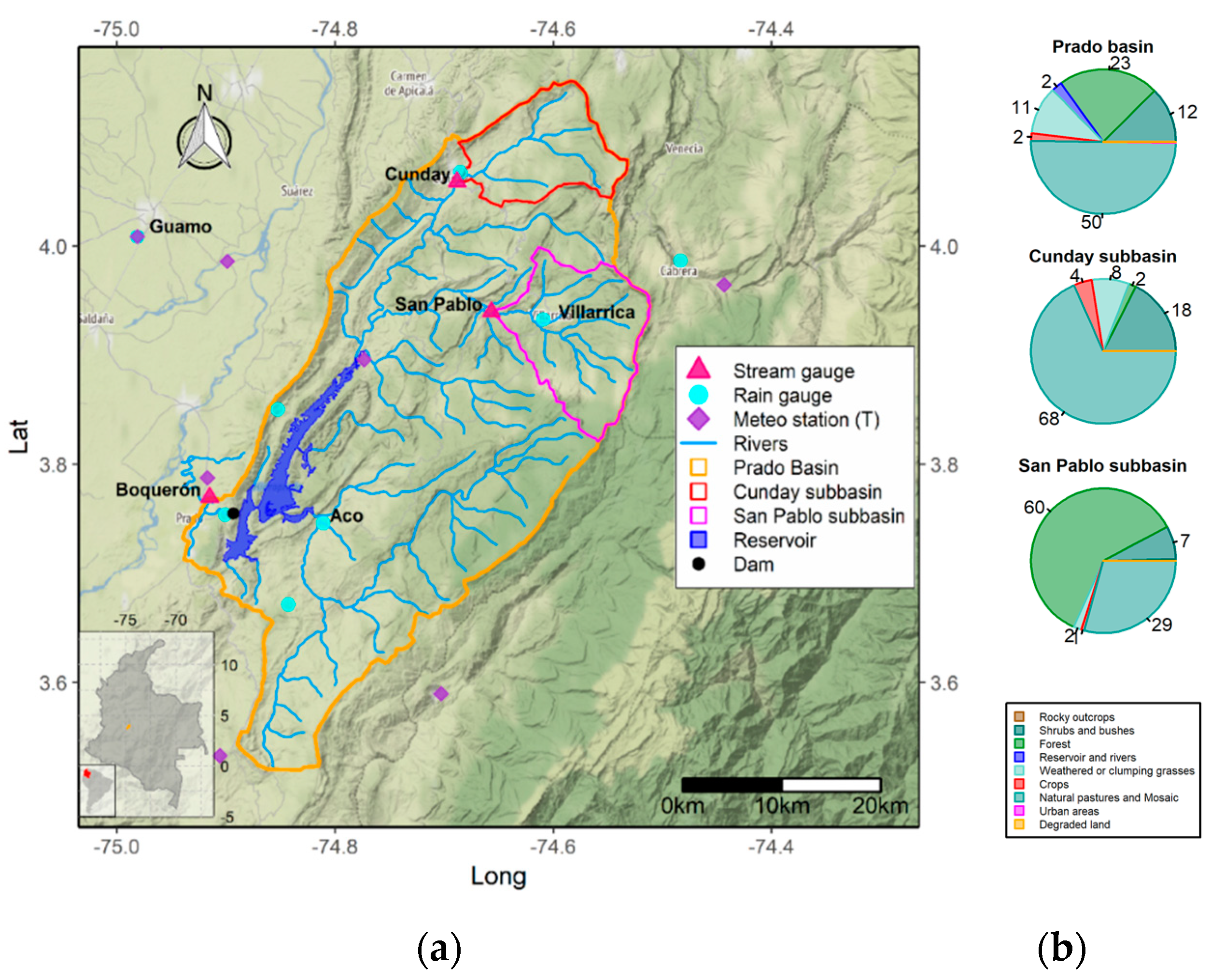
The Prado River is located in the central mountainous of Colombia. The Prado River originates in the Eastern Cordillera at an altitude of 2100 m above sea level (masl), and it flows from east to west. The longitude of the main river channel is approximately 96 km, presenting an average slope of 2% and discharging into the Magdalena River at an approximate elevation of 300 masl (Figure 1a). The basin has a mean monthly temperature (T) of 23.4 °C, oscillating between 28.1 and 17.5 °C, and P of 1895 mm year−1. Most of the monthly runoff is generated in the upstream subbasins of the Negro and Cunday Rivers. The Prado Hydroelectric Project has the fourth largest reservoir in Colombia, 42 km2 (Figure 1a). The construction of the hydroelectric project started in 1961 and was followed by the filling of the reservoir and beginning of operation in 1973. The reservoir is multiuse, providing services for electricity, irrigation, aquaculture, fishing, recreation, and tourism, and is fed by the Cunday and Negro Rivers, as well as other smaller tributaries. The hydroelectric project comprises a large dam of 56 m in height and an associated water impounded reservoir that covers 2.6% of the area of the upstream basin. The Prado Hydroelectric Project has a volume of 1100 × 106 m3 used to generate electric power with a nominal generation capacity of 60 MW that feeds into the Colombian National Electricity Grid. The reservoir also supplies water to the 2634-ha Prado River Irrigation and Drainage District located downstream of the dam. The area irrigated by the project consists mainly of rice (87%) and corn, grass for fodder and fruit trees. In addition, the reservoir supplies drinking water to 40,000 people in the Central section of the Colombian Andes [27]. According to CORINE Land Cover Colombia [28], the basin is covered in 50% by grasslands, 23% forests and 12% shrubs and bushes (Figure 1b). The Cunday River sub-basin is mainly covered by grasslands (68%), shrubs and bushes (18%), and crops (4%) and the San Pablo River sub-basin by forests (60%), grasslands (29%) and shrubs and bushes (7%).
2.2. Hydroclimatic Datasets and Processing
We collected data on discharge, precipitation and temperature in the region. We used the three discharge monitoring stations that create the Prado River Basin and its two unregulated upstream subbasins: Boquerón (main Prado Basin) and subbasins Cunday, and San Pablo, respectively, as shown in Figure 1a. The first one is located immediately downstream of the location of the dam with upstream drainage area of 1630 km2, and the second and third stations have upstream drainage areas of 131 and 174 km2, respectively. We converted the series from streamflow in m3/s to runoff (R) in mm/month or/year by dividing it by the drainage basin area. We used the calendar year for our analysis as we consider it convenient due to the tropical location of the hydrological basin. The period of runoff data availability differed among the three stations: Boquerón (1959–2002), Cunday (1954–2014) and San Pablo (1959–2014). We delineated the basin and its two sub-basins with the digital elevation model (3-arc second resolution) obtained from the EarthExplorer platform, which is hosted by the U.S. Geological Survey [31]. The drainage network shape file and the location of the three discharge monitoring stations were obtained from the web platform DHIME (in Spanish, Datos HIdrológicos y MEteorológicos) of the Colombian Institute of Hydrology, Meteorology and Environmental Studies (in Spanish, Instituto de Hidrología, Metereología y Estudios Ambientales - IDEAM) [32].
Out of the 41 meteorological stations available within and in the surroundings of the Prado River Basin, we selected the eight stations with the most complete monthly precipitation (P) data, that is, those stations that had less than 10% of monthly missing data during the period of research (i.e., 1954–2014). This information was interpolated spatially (cell size 300 × 300 m) using the inverse distance weighting interpolation method (IDW) with second power [33]. The spatially-interpolated and weighted monthly data of P was then used to calculate a monthly P average of all cells within each sub-basin of the Prado drainage basin.
The monthly T data from seven stations were obtained from IDEAM [32]. The stations had on average 33 years of monthly data with less than 5% of the data missing. One station located outside of the Prado River Basin but close to it (i.e., Guamo-21185030 with an altitude of 360 masl) had data throughout the period 1957 to 2013, with not more than 3% of missing data (Figure 1a). The missing values from 1954 to 1956 and 2014 in the time series of T in Guamo station were filled with T data from NASA Global Land Data Assimilation System (GLDAS) [34]. The GLDAS-2.0 dataset has two components: one forced entirely with the Princeton meteorological forcing data (hereafter, GLDAS-2.0) [35], and the other forced with a combination of model and observation forcing data sets (hereafter, GLDAS-2.1). The daily products of GLDAS have a 0.25 degree resolution and currently cover the period from January 1948 to December 2014 [36]. The results of this process were used to calculate T at the mean elevation of the Prado River Basin and its sub-basins by means of the thermal gradient (6.1 °C/km; [37]).
2.3. Post Processing Methods: Separation of Effects on Hydroclimatic Variables
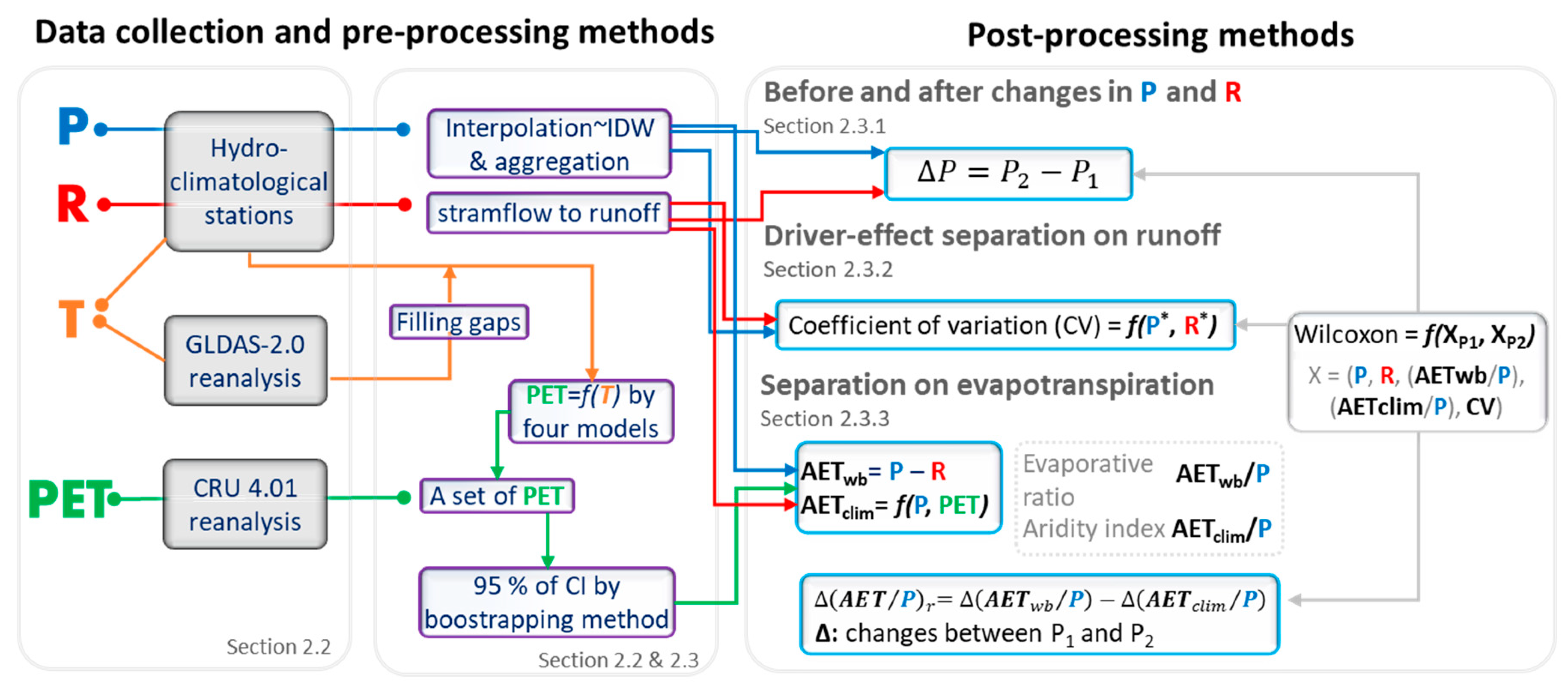
There are several driver-effect separation techniques in the literature (see review in Jaramillo [38]). In this study, we combined two simple frameworks for separating the effects of landscape and climatic drivers on evapotranspiration [39,40] and the variability of runoff [41]. We basically compared these hydrological parameters before and after the construction of the dam, and between the regulated Prado river downstream and the unregulated upstream sub-basins Cunday and San Pablo, and complemented these analyses with statistical significance tests (Table 1). The overarching framework of this study is shown in Figure 2. Furthermore, we compared the mean of the hydrological variables for the pre-dam (1954–1972) and post-dam (1973–2014) periods by means of the non-parametric Wilcoxon’s test [42]. If the resulting p-value of the Wilcoxon’s test was less than the 0.05 significance level, the null hypothesis H0 (i.e., nonidentical populations) was rejected, concluding that there was a statistically significant difference between the monthly medians in the populations before and after the construction of the dam (H1).
2.3.1. Before and After Changes in Precipitation and Runoff
In order to identify any potential effect of the reservoir on regional and local P, we studied the evolution of monthly P in the three rain gauge stations that were closest to the stream gauge stations in each sub-basin and located upstream of the dam (i.e., Aco (Prado Basin), Cunday (Cunday sub-basin) and Villarrica (San Pablo sub-basin)). We assessed changes between the periods with available hydroclimatic data before construction (Period 1–P1) 1954–1972 and after construction (Period 2–P2) 1973–2014, where the value for each period was calculated as the arithmetic mean of all annual (or monthly) values with complete data within each period (See Equation (1) for the case of precipitation). We performed the same procedure for multiannual monthly and annual runoff averages.
Separating the effects of an impounded reservoir on precipitation can only be done with complex modelling such as that of moisture tracking, either by the Lagrangian (e.g., [43]) or Eulerian approaches (e.g., [44,45]) or by a spatial sample with several reservoirs and stations. Since the scarcity of data in the region does not allow for this analysis, we limited ourselves to the comparison of monthly total precipitation before and after the impoundment of the reservoir and the multi-comparison of these differences across the regulated basin and its subbasins.
2.3.2. Driver-Effect Separation on Runoff Variability
We studied the evolution of the inter-annual monthly variability of P and R throughout the available period by calculating the coefficient of variation of precipitation (CVP) and runoff (CVR), respectively, in order to detect any changes in intra-annual variability of these variables before and after the construction of the hydroelectric project. We assumed that the coefficient of variation of precipitation can be used as a proxy of the climatic or natural variability of runoff at the interannual scale, following Jaramillo and Destouni [41]. The effect of regulation on the variability of runoff can then be obtained by comparing: (1) CVR before and after the impoundment of the reservoir, and (2) the relationship between CVR and CVP before and after impoundment, and (3) 1 and 2 between the regulated hydrological basin and the two unregulated subbasins. The coefficient of variation is the standard deviation of the 12 monthly values divided by their annual mean. As such, a time series is more homogeneous for low values of the coefficient of variation. In order to reduce the high inter-annual variability of R and P for the time series analysis and identify more clearly any long-term changes, we applied a ten-year moving window filter to each of the time series. We further tested other calculations of CVR and CVP by using a twelve-month CVR and also a sixty-month CVR, and then moving the CV calculation each month.
2.3.3. Separation on Evapotranspiration
Regional evapotranspiration data can be taken from satellite observations, although the available periods are generally too short (i.e., since 2000) [46]. Otherwise, the water mass balance can be used to estimate the AET of a basin by using mean basin-scale P and R over long periods of time and assuming a negligible change in water storage within the basin over the period of analysis, providing an overview of the net effect of all drivers of evapotranspiration (Equation (2)) [47,48,49]. However, the water balance method by itself does not provide additional information about the drivers of change in evapotranspiration due to the large number of interacting drivers in a given basin [50]. We refer to this actual evapotranspiration calculation as AETwb (Equation (2)).
The Budyko empirical equation expresses the evaporative ratio (i.e., AET/P) in terms of potential evapotranspiration (PET) over precipitation, also named the aridity index (i.e., PET/P). It can be used to obtain a climatic estimate of the annual evapotranspiration, which in this case is solely dependent on PET and P calculations and data, respectively ([51,52]) (Equation (3)). We refer to this second estimate ([51]) of AET as the climate-driven AET, AETclim.
For the use of Equation (3), we initially used a PET raster product from the Climatic Research Unit (CRU-TS 4.01), at a spatial resolution of 0.5° (UEA CRU et al., 2017). This last set of PET data is a variant of the Penman–Monteith FAO method (FAO: Food and Agriculture Organization) (Ekström et al. [53], based on Allen et al. [54]), which uses average temperature Tmin, Tmax, vapor pressure, cloud cover, and wind speed, based on fixed weather conditions [55]. We also estimated PET based on other temperature and radiation-dependent equations, for which information was available (Table 2; Hargreaves–Samani [56], Hamon [57], Blaney–Criddle [58] and Langbein [59]). For the case of the Hargreaves–Samani, radiation data were computed based on latitude and month.
Lastly, we quantified the change in the residual evaporative ratio between the two periods, Δ(AET/P)r, as shown in Equation (4), since other studies have found that a positive Δ(AET/P)r can be an indicator of the effect of water use within a given basin on the evaporative ratio, specifically by increasing evapotranspiration related to irrigation and/or impoundment of reservoirs [18,19,60]. Hence, Δ(AET/P)r represents the component of the change in the evaporative ratio that is not explained by variability in potential evapotranspiration and/or precipitation, and as such represents the change component of any other driver of change related to changes in the surface such as changes in vegetation, water use, or soil characteristics, that may change the rates of evapotranspiration in the basin. In this case, Δ(AETclim/P) and Δ(AETwb/P) were calculated in the same manner as in Equation (1).
The nature of the change on Δ(AETwb/P) and Δ(AETclim/P) is based on the parameters used for their calculation. A positive Δ(AETwb/P) can really relate to anything that increases AET and decreases R (Equation (2)), either climatic or stemming from changes in land cover, vegetation, land use, etc., or based in this framework, anything that affects Δ(AETwb/P) or Δ(AET/P)r. That is why it is important to also calculate Δ(AETclim/P), the latter relating only to the effect of climatic parameters on the evaporative ratio, more specifically P and PET. It is worth noting that the calculation of PET depends in turn on several other climatic parameters such as relative humidity, wind speed, temperature and radiation, depending on the model used (See Table 2). Hence, a positive Δ(AETclim/P) can relate to an increase in PET—by either an increase in wind speed, in temperature, in radiation, or a decrease in P (see the structure of Equation (3)).
The change in residual can explain the driving effect of human activities on evapotranspiration change, or in our case, change in the evaporative ratio of a basin. For instance, if the Δ(AET/P)r is positive, it implies that Δ(AETwb/P) is larger than Δ(AETclim/P), and as such, the driver of the residual must have increased AET, considering that P is the same for all estimates. Drivers that can then increase AET include a change in land cover related to vegetation (i.e., grassland to forest or non-irrigated to irrigated crops systems) or to water (i.e., change of grassland to water surface when constructing an impounded reservoir). Conversely, a negative Δ(AET/P)r can then point to decreasing AET from deforestation due to less biomass and vegetation coverage.
3. Results
3.1. Detecting Changes in Precipitation and Runoff
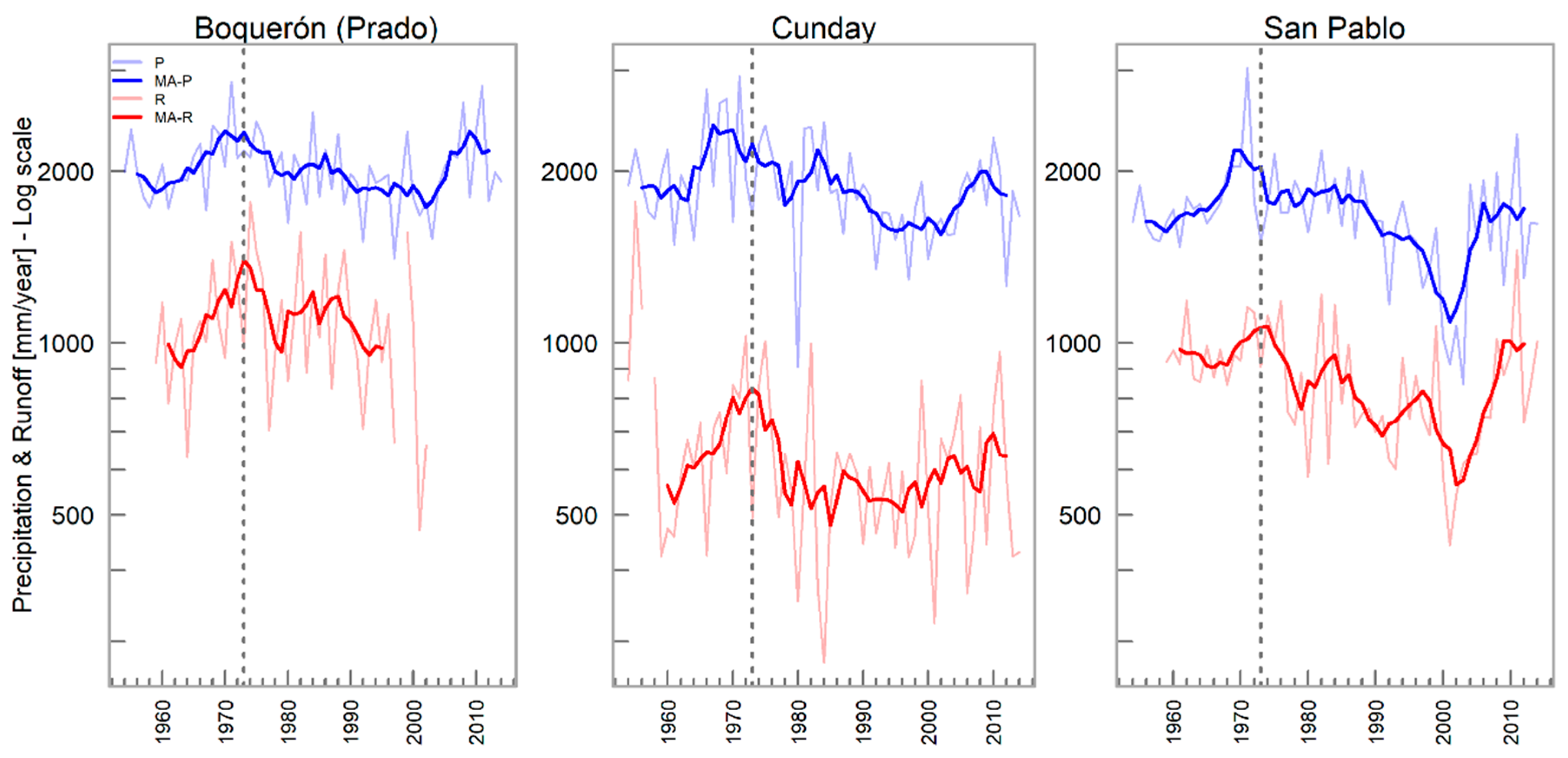
The time series analysis shows an inter-annual variation pattern that is similar for P and R, both on basin (Prado measured at Boquerón station) and sub-basin scales (measured at Cunday and San Pablo stations) (Figure 3). Furthermore, a simultaneous decrease in P and R occurs after the time of commissioning of the project in 1973. If the continuous decrease in P and R would have occurred only in the Boquerón station and not in the two sub-basins located upstream, it could be indicative of the effects of the commissioning of the project. However, since the decrease is more regional than local, also occurring in the two sub-basins located upstream of the Prado reservoir, it is more likely that the decrease in P and a large part of the decrease in R are driven by climatic variability. During the studied period, the sub-basin of San Pablo reported the lowest annual mean of P (1676 mm year−1), in comparison to Cunday sub-basin and Prado Basin (1885 mm year−1 and 2021 mm year−1, respectively). The mean annual runoff for the Cunday sub-basin (635 mm year−1) was also less than the value calculated for San Pablo (860 mm year−1), meaning that although it might rain more in Cunday than in San Pablo, the amount of precipitation that partitions into runoff is less.
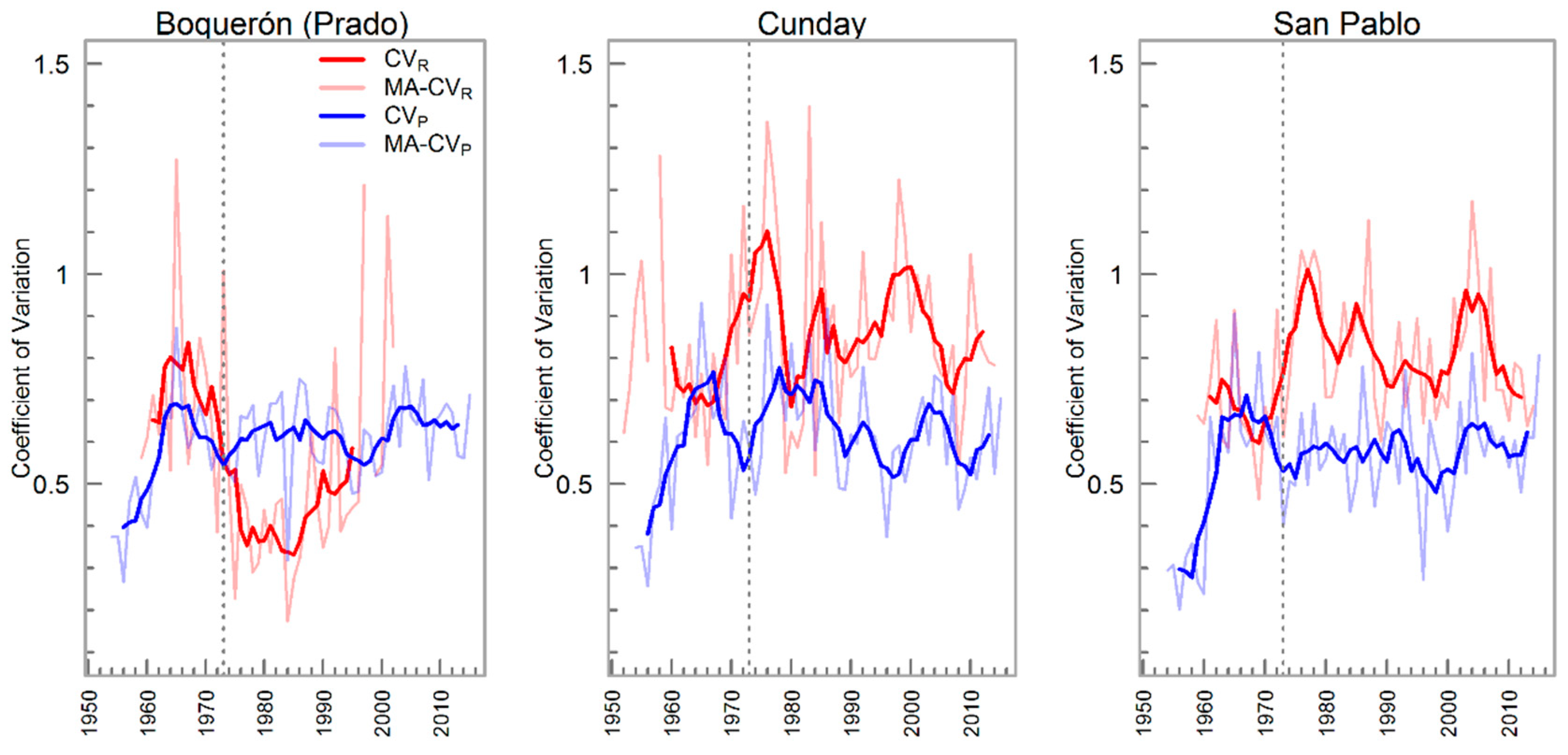
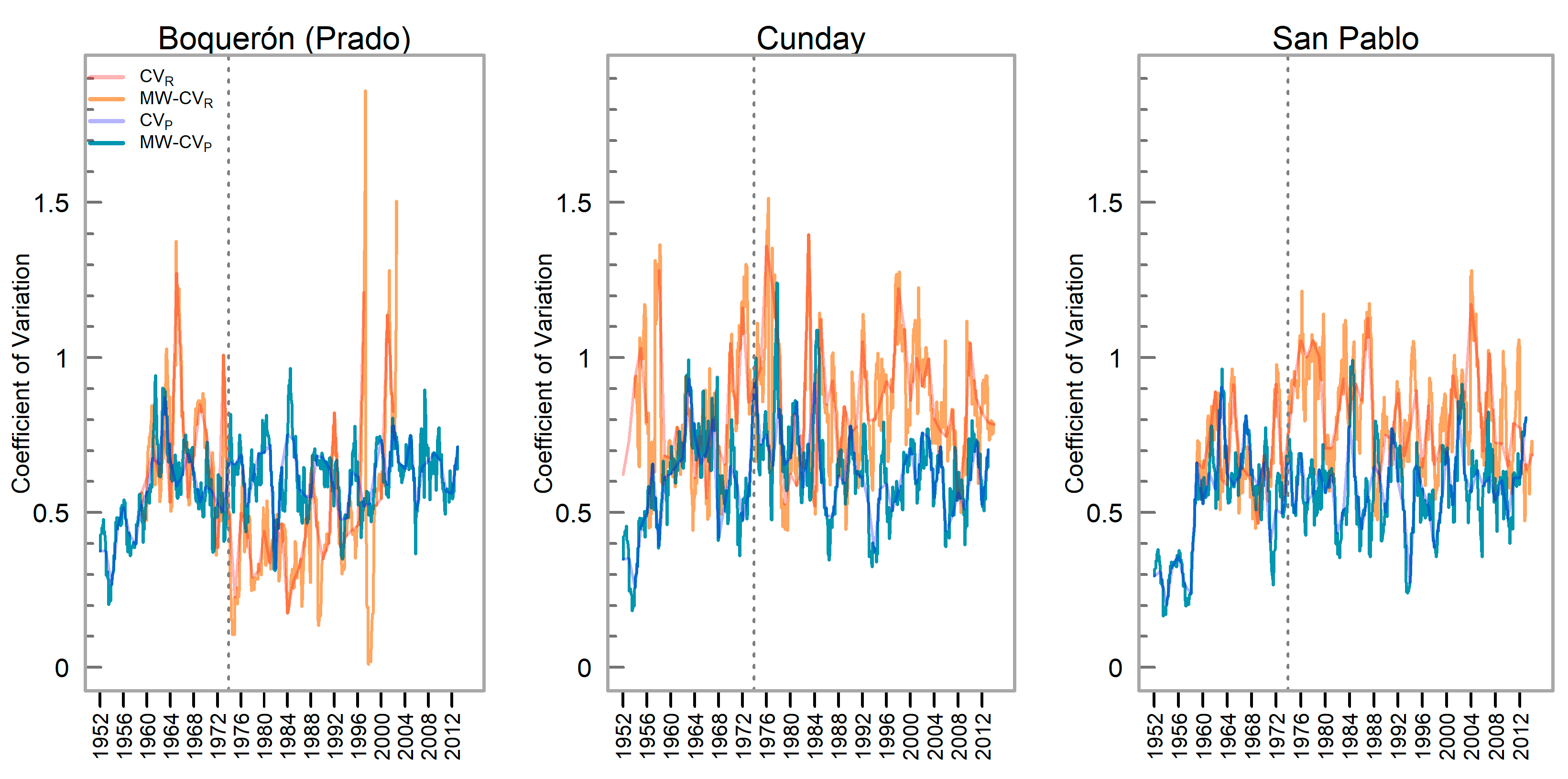
Regarding the annual variability of precipitation, the coefficient of variation of precipitation (CVP) over Prado, Cunday and San Pablo basins followed the same temporal pattern; an increase around 1968 and a stabilization, with minor oscillations, after this period (Figure 4) without any clear difference among the three basins or indication of the effect of the reservoir in precipitation variability. Rather, the precipitation variability in the region is generally associated with the interactions between the intertropical confluence zone (i.e., between 4° and 7° latitude), orography and local circulation, which affect the volumes of precipitated water [61]. As opposed to CVP, the overall trend of CVR in Boquerón (Prado Basin) is markedly different from that of Cunday and San Pablo and quite different before and after the hydroelectric power plant began operations. In the period before 1973, all stations show a similar CVR, but after 1973, CVR in Boquerón (Prado Basin) decreases while that of San Pablo and Cunday sub-basins increase. In addition, CVR after 1973 oscillates in a lower level in Boquerón than in the two sub-basins, meaning that the differences in R between the twelve months have decreased by the flow regulation of the dam. This can be also seen for the variability of total monthly runoff (Figure 5). These results are similar regardless of the methods of computation of CV (See Supplementary Materials, Figure A1 and Figure A2).
To test whether the CVP and CVR were significantly similar in the basin and its sub-basins, the Wilcoxon contrast method was used (Table 3) between the periods before and after the construction of the dam. We found that the only significant difference (p < 0.05; Wilcoxon) among basins existed for the median values of CVR for the period after the construction of the dam between Cunday and Boquerón (Prado Basin) and San Pablo and Boquerón (Prado Basin) stations, pointing to an effect of flow regulation. For the case of CVP, significant differences (p < 0.05; Wilcoxon) were found between Prado and Cunday in the period after the construction of the dam. The significant differences of CVP between the two upstream sub-basins are possibly due to the difference in precipitation patterns among them according to their specific orographic characteristics. However, the magnitude and direction of the CVP’s from Prado and San Pablo were significantly different (p < 0.05). This result can be related to monthly variability of P in San Pablo has been different from values observed in Cunday before and after the construction of the dam. To validate the differences between the CVP’s of San Pablo with Prado and Cunday, the contrast tests of the MK, Sen’s slope and Levene, were applied on a monthly scale to rule out possible effects of the relative variability of the CV. In general, we estimate that the impoundment of the reservoir has decreased CVR by 33%, after removing the change in natural variability as observed in the development of CVR from the period before the dam to the period after.
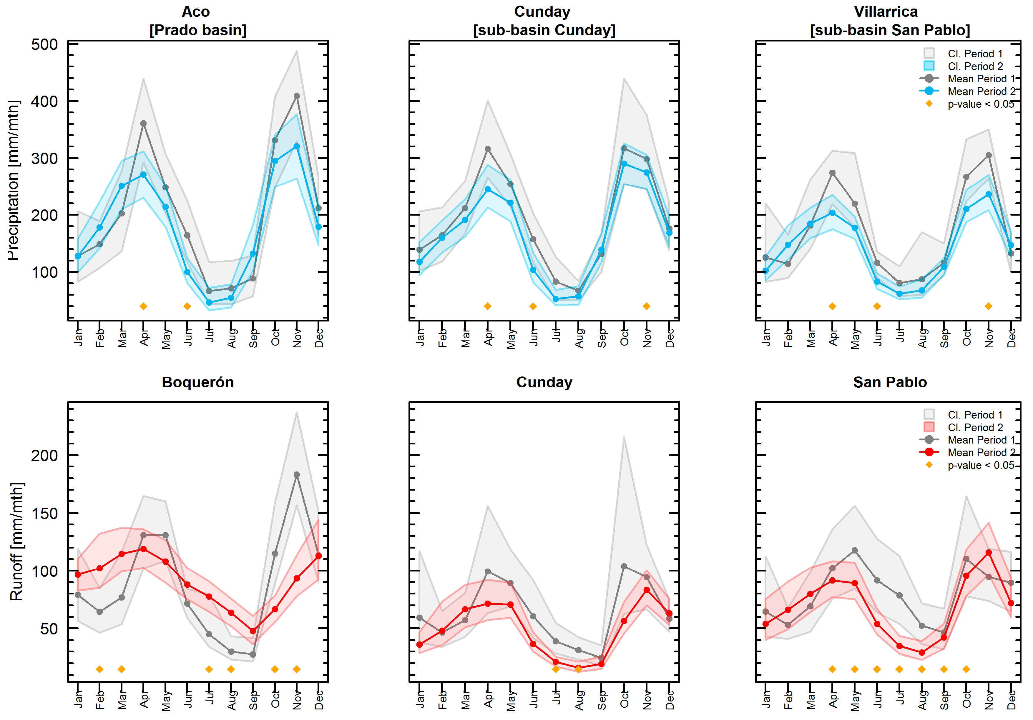
An analysis of the average monthly R and P in the Prado Basin and its sub-basins (Cunday and San Pablo) gives more insight into the reasons behind the changes of CVR and monthly R occurring in Boquerón station after the regulation of the Prado River in 1973 (Figure 5). Firstly, after the construction of the dam and during the dry period stretching from June to September, the regulation of the dam produced more runoff in Boquerón (Prado basin) than the actual amount of precipitation falling within its upstream basin. This only occurs in the Boquerón (Prado basin) station and is not observed in the other two discharge stations corresponding to the sub-basins upstream. Secondly, while the seasonal pattern between monthly P and R is consistent before and after the construction of the dam in the upstream Cunday sub-basin (i.e., they are in phase), the seasonal pattern of R is consistent with that of P only before the construction of the dam in the Prado Basin. This explains how the Prado reservoir retains water during the wet season of March to May and October to December to maximize the reservoir capacity for hydropower generation, to later release it in the dry period from June to August.
Furthermore, the monthly confidence intervals (CI) of P (Figure 5) show a reduction in the magnitude and variance of this variable during P2 (blue) with respect to P1 (gray) during the wettest months (April and November) and in the dry month of June. Although the reduction in P in these months could be attributed to the construction of the dam, the fact that it occurs also over the upstream subbasins suggests that these decreases are more related to natural climatic variability.
3.2. Main Hydroclimatic Changes in the Basins
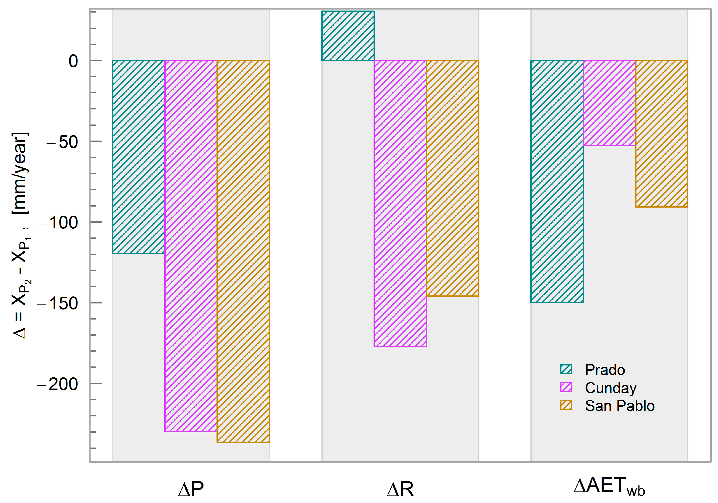
Now, when studying simultaneously the changes in the means of R, P, and AET between P1 and P2 for the Prado basin and the two sub-basins, we found that P had decreased in the three basins. In the sub-basins Cunday and San Pablo, the decrease in P partitioned mostly into a decrease in R than a decrease in AETwb (Figure 6). For the case of the large Prado basin including the reservoir, the decrease in P of 120 mm year−1 partitioned mostly into a decrease in AETwb of 150 mm year−1 and an increase in R of 30 mm year−1. Contrary to basin-wise analysis in regulated basins that have found an increase in AETwb after regulation, the Prado regulated basin experienced a decrease in AETwb, highlighting the potential role of other drivers of AET change that tend to reduce evapotranspiration or the negligible effect of the reservoir on evapotranspiration at the basin scale (See Figure A4).
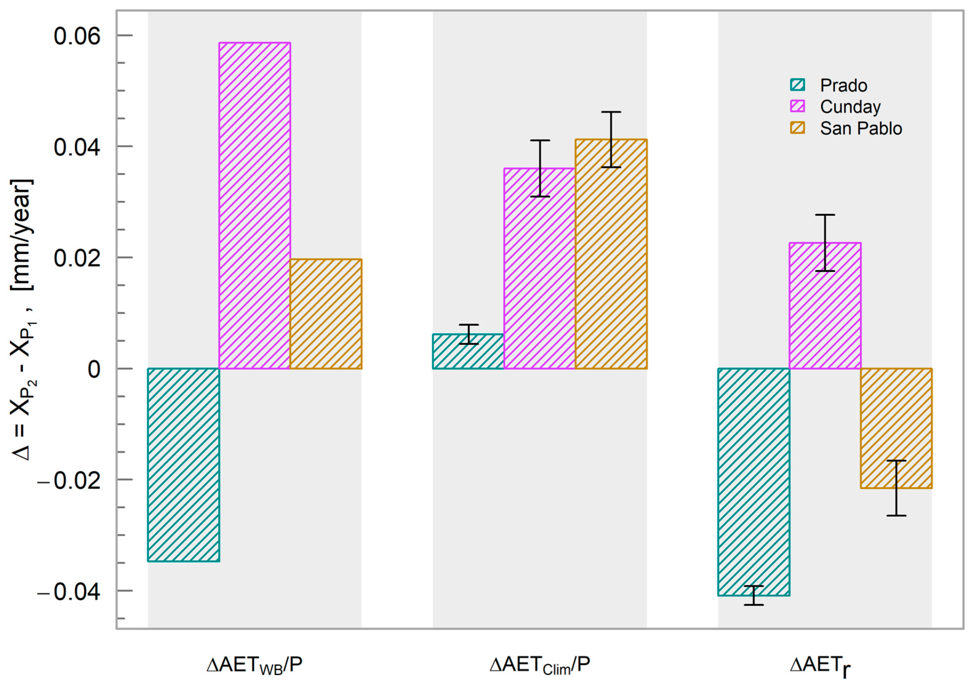
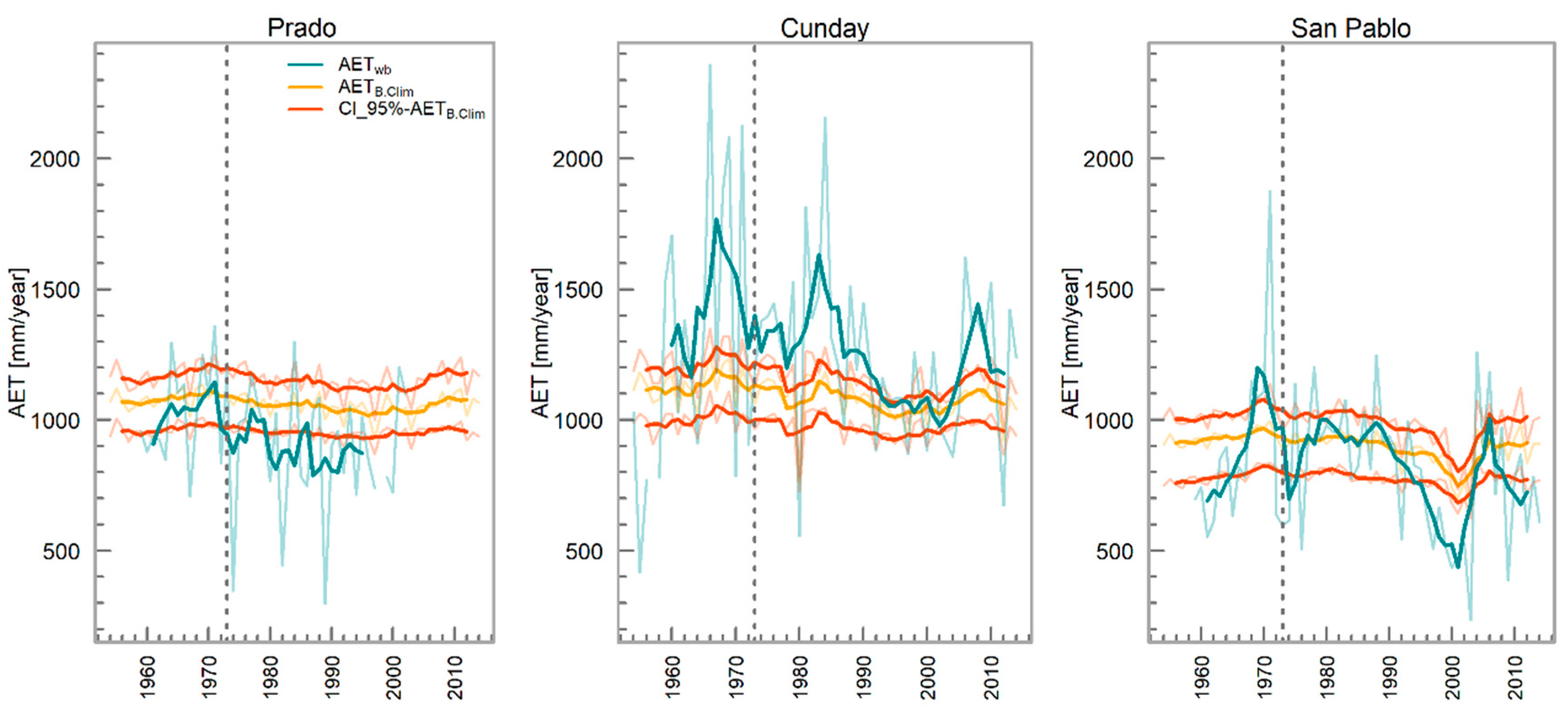
To verify if these basin-scale mean annual changes may be related to the impoundment of the reservoir and not to precipitation and/or PET changes, we analyzed the time series of AETwb/P and AETclim/P and calculated the residual Δ(AET/P)r (Figure 7). The AETwb/P in Prado has been generally below the mean and CI values of AETclim/P in both periods. On the other hand, in the Cunday sub-basin, the AETwb/P has been over the AETclim/P throughout the analysis period, but both the magnitude and the direction of the tendencies are significantly similar before and after 1973 (p < 0.05). Although the rates and variability of P in Cunday are similar to those observed in San Pablo and Prado, there is a greater evapotranspiration in Cunday (see Figure A3), possibly due to the higher mean temperature (i.e., 25 °C in Cunday and 21 °C in San Pablo).
The residual change Δ(AET/P)r gives information on the other possible governing drivers of evapotranspiration change in the basin, with the sign and the magnitude of the change providing information on the nature of the main drivers different from PET or P such as other climatic factors, land or water use [63]. As Δ(AET/P)r is negative in the Prado River basin, there appears to be no effect of the impoundment of the reservoir on evapotranspiration, or at least is shadowed by other effects. Furthermore, Δ(AET/P)r is positive in its upstream unregulated subbasin, highlighting even more the lack of the expected signal from the reservoir.
4. Discussion
Since the long-term changes in the variables here studied may be driven by a combination of inter-annual and intra-annual climate variability and other factors such as deforestation [64], reforestation [63], rainfed and irrigated agricultural development [65] and impoundment of water in reservoirs [66], it is difficult to attribute these changes to a sole driver. However, changes in the hydrologic variables before and after the construction of the dam could suggest or at least point to a possible influence of the project on the basin’s long-term hydroclimate. Such methodology has been used to study the effects of forestry, rainfed agriculture and hydropower development on the hydroclimate of a given basin (e.g., [18,19,60,63]).
The current results show a decrease in CVR by 33% that is explained by the regulation of the reservoir. This effect was not observed in the sub-basins upstream from the project. Regarding the change in precipitation and runoff observed in the basin and its subbasins, if the decreasing trend of precipitation and runoff continue in the Prado River Basin in the future, the operation of the hydroelectric project might be affected when compared to its current conditions, although more information is needed regarding the operation of the dam that in this case is confidential and not distributed by the operating company.
Furthermore, the need to release runoff resulting from the wet season (i.e., March, April, October, and November) to keep the storage for flood control means that the vulnerability to water security as ecosystem service downstream during the dry season will increase. In order to compensate this imbalance between the availability of water during the wet and dry months, the dam administrators must retain more water than what is naturally available in the rivers during the wet season, and release a greater amount of water stored during the dry season, as evidenced by Ehsani et al. [67] in regulated dams in the northeastern United States.
Hydropower production developments have been reported to co-occur with a AETwb/P increase and a CVR decrease [18,19,60]. However, the novelty of our study in a tropical regulated basin relies in the fact that only changes in CVR were here found, and not the increase in evaporative ratio expected from regulated reservoirs as seen in other Mediterranean, boreal and temperate regulated basins. This may be explained by the fact that the construction of only one reservoir within the basin may not be sufficient to evidence an effect on net evapotranspiration from flow regulation from the entire basin. On the other hand, a physical interpretation of the finding is related to the sensible and latent heat fluxes for open water bodies and vegetated covers. In tropical and humid regions, forested areas exhibit comparable moisture fluxes due to transpiration than evaporation from open water bodies [12]. Therefore, flooding or clearing of forest by an artificial lake are unlikely to create a distinctly different local climate. However, in semi-arid, Tundra, humid continental and Mediterranean regions, several studies [4,18,19,40] have demonstrated that the reservoirs can to add sufficiently more moisture than the sparsely vegetated surroundings, resulting in spatial gradients of water vapor flux in these types of climate. Although the reservoir in the Prado River basin has the characteristics of a large dam, the monthly precipitation magnitude and variability in the Prado basin and its subbasins Cunday and San Pablo appear not to be affected in this case.
Another possible uncertainty might be related to the limited availability of climatic data on wind speed and radiation, variables needed to calculate a more precise value of PET. The lack of specific humidity, radiation, moisture and wind, data for the region and during the time of construction of the dam does not allow us to specify which may be the most relevant climatic parameter. Not accounting for these factors based on the lack of measured data may also be linked to the decrease in relative actual evapotranspiration. Other driver-effects occurring in the basin may also be reasons why an increase in (AET/P)r is not observed. Furthermore, since deforestation in the basin should decrease (AET/P)r as here found, [68], deforestation may also be a factor changing evapotranspiration and the evaporative ratio before and after impoundment.
5. Conclusions
For the regulated tropical river basin here studied, we found a decrease in the long-term coefficient of variation of runoff as seen in other regulated basins around the world. However, we did not find changes in precipitation (both monthly and annual scales) or the expected increasing evaporative ratio-effect (annual scale) from the impoundment of the reservoir, founding for the latter rather a decrease. This may be due to the humid conditions of the region where actual evapotranspiration is already close to its potential or to other land cover changes that decrease evapotranspiration during the studied period. Our study shows that the effects from impounded reservoirs in tropical regulated basins may differ from those found in other climatic regions.
Supplementary Materials
The following are available online at https://0-www-mdpi-com.brum.beds.ac.uk/2071-1050/12/17/6795/s1, Excel S1: Evaporation Data, Excel S2: Precipitation Data, Excel S3: Stream Flow Data, Excel S4: Temperature Data, Zip S5: Temperature Data From GLDAS.
Author Contributions
D.Z. analyzed the data and drafted the manuscript. F.J. edited the manuscript and revised the statistical results. E.R. contributed to editing and organizing the manuscript. All authors reviewed the article. All authors have read and agreed to the published version of the manuscript.
Funding
This research study was funded by: (1) No. 647 scholarship program of the Administrative Department of Science, Technology, and Innovation—Colciencias, Colombia, (2) the Doctoral Studies Support Program a joint project between the Center for Development Research at the University of Bonn, Germany, and the Environmental Studies Institute at the Universidad Nacional de Colombia and funded by German Academic Exchange Service (DAAD—Federal Ministry of Economic Cooperation and Development), (3) the Swedish Research Council (VR, project 2015-06503) and 4) the Swedish Research Council for Environment, Agricultural Sciences and Spatial Planning FORMAS (942-2015-740).
Conflicts of Interest
The authors declare no conflict of interest.
Appendix A
Figure A1.
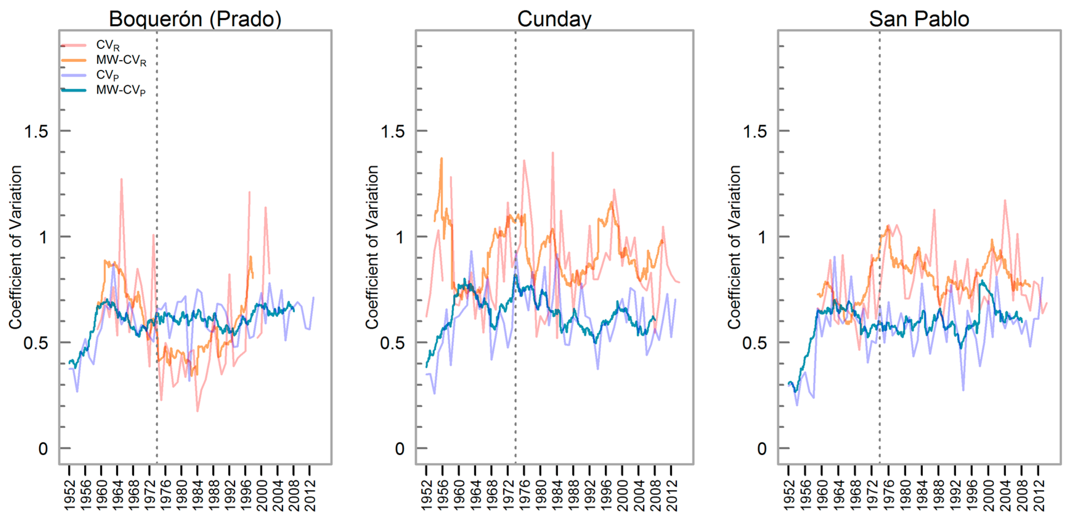
Coefficient of variation of monthly runoff (CVR; red) and precipitation (CVP; blue) and moving window (MW) using twelve months to calculate CV for runoff (MV-CVR; orange) and precipitation (MV-CVP; darkblue) in the Prado River Basin (Boquerón) and its two sub-basins (Cunday and San Pablo).
Figure A1.
Coefficient of variation of monthly runoff (CVR; red) and precipitation (CVP; blue) and moving window (MW) using twelve months to calculate CV for runoff (MV-CVR; orange) and precipitation (MV-CVP; darkblue) in the Prado River Basin (Boquerón) and its two sub-basins (Cunday and San Pablo).

Figure A2.
Coefficient of variation of monthly runoff (CVR; red) and precipitation (CVP; blue) and moving window (MW) using 60 months to calculate CV for runoff (MV-CVR; orange) and precipitation (MV-CVP; darkblue) in the Prado River Basin (Boquerón) and its two sub-basins (Cunday and San Pablo).
Figure A2.
Coefficient of variation of monthly runoff (CVR; red) and precipitation (CVP; blue) and moving window (MW) using 60 months to calculate CV for runoff (MV-CVR; orange) and precipitation (MV-CVP; darkblue) in the Prado River Basin (Boquerón) and its two sub-basins (Cunday and San Pablo).

Figure A3.
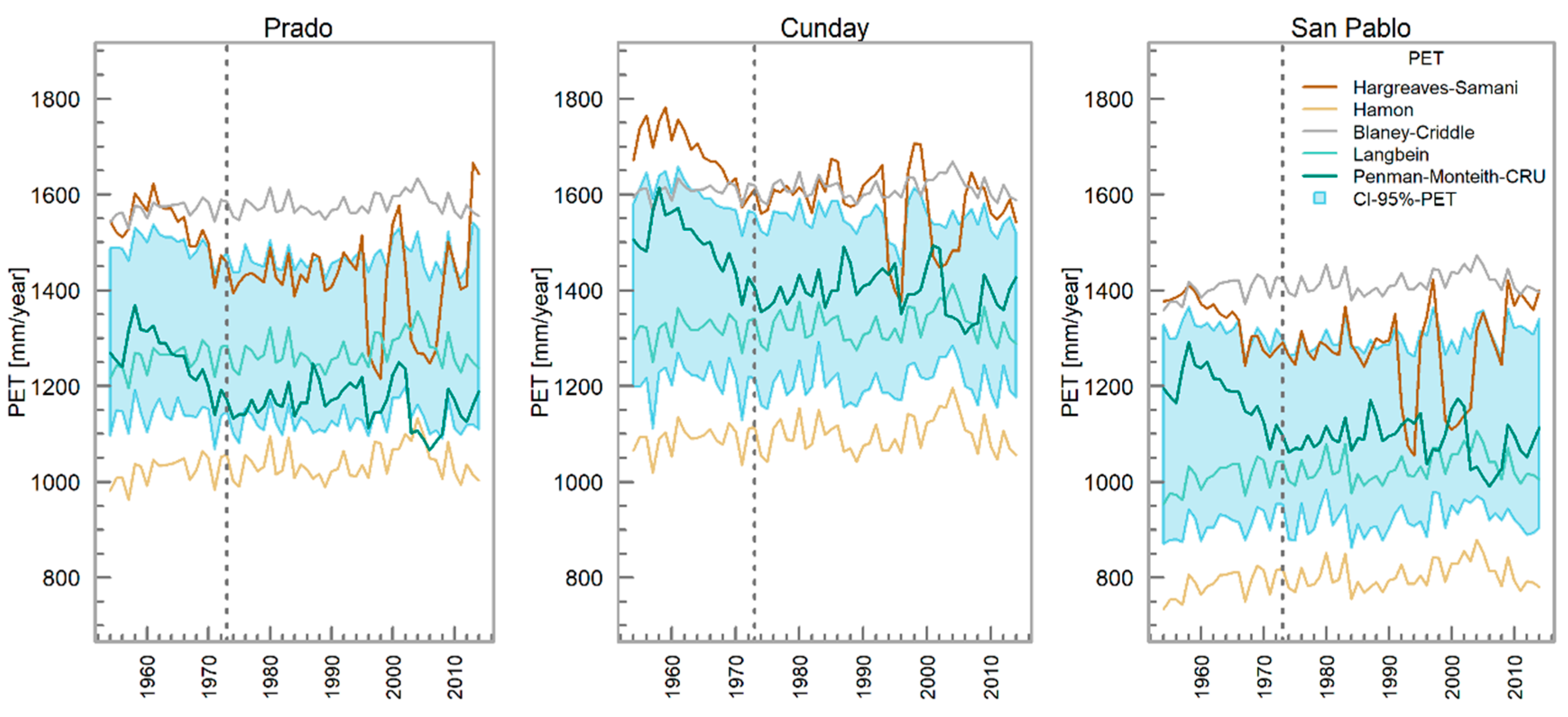
Annual potential evapotranspiration (PET) estimated by five different models and its 95% confidence intervals (CI) from 1954 to 2014. The CIs were calculated using the non-parametric bootstrap bias-corrected and accelerated [62] with 2000 bootstrap replicas for each of the months within the study periods.
Figure A3.
Annual potential evapotranspiration (PET) estimated by five different models and its 95% confidence intervals (CI) from 1954 to 2014. The CIs were calculated using the non-parametric bootstrap bias-corrected and accelerated [62] with 2000 bootstrap replicas for each of the months within the study periods.

Figure A4.
Changes in the water balance-based actual evapotranspiration (AETwb) and estimated evapotranspiration based on a yearly climate approach (AETclim) from 1954 to 2014, presented through a 10-year moving average in the Prado River Basin and its sub-basins. The gray dotted line shows the year in which the hydroelectric plant began operations (1973). The red lines are the CIs of AETclim and were calculated using the non-parametric bootstrap bias-corrected and accelerated [62] with 2000 bootstrap replicas for each of the months within the study periods.

Appendix B
We compared the PET from Langbein model with pan evaporation (PE) measures from the Guamo meteorological station (see Figure 1a). The PE records are available from 1965 to 2012 with 22% of missing data on a monthly scale. Therefore, we considered the 21 years without monthly missing data of PE and aggregate them into an annual scale and finally compared them with PET. The mean interannual values of PE and PET were 1714 and 1604 mm year−1, respectively, and the standard deviation among these variables was around 155 mm year−1.
References
- Falkenmark, M.; Wang-Erlandsson, L.; Rockström, J. Understanding of water resilience in the Anthropocene. J. Hydrol. X 2019, 2, 100009. [Google Scholar] [CrossRef]
- Vörösmarty, C.J.; Sahagian, D. Anthropogenic Disturbance of the Terrestrial Water Cycle. Bioscience 2000, 50, 753. [Google Scholar] [CrossRef] [Green Version]
- Solomon, S.; Qin, D.; Manning, M.; Averyt, K.; Marquis, M. Climate Change 2007—The Physical Science Basis: Working Group I Contribution to the Fourth Assessment Report of the IPCC; IPCC: Geneva, Switzerland, 2007. [Google Scholar]
- Jaramillo, F.; Destouni, G. Comment on “Planetary boundaries: Guiding human development on a changing planet”. Science 2015, 348, 2015–2017. [Google Scholar] [CrossRef] [PubMed] [Green Version]
- Woldemichael, A.T.; Hossain, F.; Pielke, R.; Beltrán-Przekurat, A. Understanding the impact of dam-triggered land use/land cover change on the modification of extreme precipitation. Water Resour. Res. 2012, 48. [Google Scholar] [CrossRef] [Green Version]
- Elliott, J.; Deryng, D.; Müller, C.; Frieler, K.; Konzmann, M.; Gerten, D.; Glotter, M.; Flörke, M.; Wada, Y.; Best, N.; et al. Constraints and potentials of future irrigation water availability on agricultural production under climate change. Proc. Natl. Acad. Sci. USA 2013, 111, 3239–3244. [Google Scholar] [CrossRef] [PubMed] [Green Version]
- Gudmundsson, L.; Tallaksen, L.M.; Stahl, K.; Fleig, A.K. Low-frequency variability of European runoff. Hydrol. Earth Syst. Sci. 2011, 15, 2853–2869. [Google Scholar] [CrossRef] [Green Version]
- Petts, G.E.; Gurnell, A.M. Dams and geomorphology: Research progress and future directions. Geomorphology 2005, 71, 27–47. [Google Scholar] [CrossRef]
- Stevaux, J.C.; Martins, D.P.; Meurer, M. Changes in a large regulated tropical river: The Paraná River downstream from the Porto Primavera Dam, Brazil. Geomorphology 2009, 113, 230–238. [Google Scholar] [CrossRef]
- Poff, N.L.; Zimmerman, J.K.H. Ecological responses to altered flow regimes: A literature review to inform the science and management of environmental flows. Freshw. Biol. 2010, 55, 194–205. [Google Scholar] [CrossRef]
- Angarita, H.; Wickel, A.J.; Sieber, J.; Chavarro, J.; Maldonado-Ocampo, J.A.; Guido, A.H.-R.; Delgado, J.; Purkey, D. Basin-scale impacts of hydropower development on the Mompós Depression wetlands, Colombia. Hydrol. Earth Syst. Sci. 2018, 22, 2839–2865. [Google Scholar] [CrossRef] [Green Version]
- Degu, A.M.; Hossain, F.; Niyogi, D.; Pielke, R.; Shepherd, J.M.; Voisin, N.; Chronis, T. The influence of large dams on surrounding climate and precipitation patterns. Geophys. Res. Lett. 2011, 38, 1–7. [Google Scholar] [CrossRef]
- Hossain, F. Empirical Relationship between Large Dams and the Alteration in Extreme Precipitation. Nat. Hazards Rev. 2010, 11, 97–101. [Google Scholar] [CrossRef]
- Zhao, Q.; Liu, S.; Deng, L.; Dong, S.; Yang, J.; Wang, C. The effects of dam construction and precipitation variability on hydrologic alteration in the Lancang River Basin of southwest China. Stoch. Environ. Res. Risk Assess. 2012, 26, 993–1011. [Google Scholar] [CrossRef]
- Jackson, R.B.; Jobbágy, E.G.; Avissar, R.; Roy, S.B.; Barrett, D.J.; Cook, C.W.; Farley, K.A.; Le Maitre, D.C.; McCarl, B.A.; Murray, B.C. Trading Water for Carbon with Biological Carbon Sequestration. Science 2005, 310, 1944–1947. [Google Scholar] [CrossRef] [PubMed] [Green Version]
- Fisher, J.B.; Tu, K.P.; Baldocchi, D.D. Global estimates of the land-atmosphere water flux based on monthly AVHRR and ISLSCP-II data, validated at 16 FLUXNET sites. Remote Sens. Environ. 2008, 112, 901–919. [Google Scholar] [CrossRef]
- Nemani, R.R.; Keeling, C.D.; Hashimoto, H.; Jolly, W.M.; Piper, S.C.; Tucker, C.J.; Myneni, R.B.; Running, S.W. Climate-driven increases in global terrestrial net primary production from 1982 to 1999. Science 2003, 300, 1560–1563. [Google Scholar] [CrossRef] [Green Version]
- Destouni, G.; Jaramillo, F.; Prieto, C. Hydroclimatic shifts driven by human water use for food and energy production. Nat. Clim. Chang. 2013, 3, 213–217. [Google Scholar] [CrossRef]
- Levi, L.; Jaramillo, F.; Andričević, R.; Destouni, G. Hydroclimatic changes and drivers in the Sava River Catchment and comparison with Swedish catchments. Ambio 2015, 44, 624–634. [Google Scholar] [CrossRef] [Green Version]
- Wang, D.; Hejazi, M. Quantifying the relative contribution of the climate and direct human impacts on mean annual streamflow in the contiguous United States. Water Resour. Res. 2011, 47. [Google Scholar] [CrossRef] [Green Version]
- Peters, T. Water Balance in Tropical Regions. In Tropical Forestry Handbook; Springer: Berlin/Heidelberg, Germany, 2016; pp. 391–403. [Google Scholar]
- Band, L.E.; Hwang, T.; Hales, T.C.; Vose, J.; Ford, C. Ecosystem processes at the watershed scale: Mapping and modeling ecohydrological controls of landslides. Geomorphology 2012, 137, 159–167. [Google Scholar] [CrossRef]
- XM Capacidad Efectiva por Tipo de Generación. Available online: http://paratec.xm.com.co/paratec/SitePages/generacion.aspx?q=lista (accessed on 6 June 2019).
- Instituto de Hidrología, Meteorología y Estudios Ambientales. Estudio Nacional del Agua 2018; IDEAM: Bogotá, Colombia, 2019; ISBN 9789585489127.
- Unidad de Planeación Minero Energética. Plan Energético Nacional, Unidad de Planeación Minero Energética; UPME: Bogotá, Colombia, 2015.
- IHA. Hydropower Status Report—Sector Trends and Insights; IHA: London, UK, 2018. [Google Scholar]
- Corporación Autónoma Regional del Tolima. Proyecto Plan de Ordenación y Manejo de la Cuenca (POMCA) Hidrográfica Mayor del Río Prado; CORTOLIMA: Ibague, Colombia, 2002. Available online: https://www.cortolima.gov.co/contenido/fase-ii-diagnostico-r%C3%ADo-prado (accessed on 22 August 2018).
- IDEAM; IGAC; CORMAGDALENA. Mapa de Cobertura de la Tierra Cuenca Magdalena-Cauca, Metodología Corine Land Cover Adaptada para Colombia, Escala 1:100.000; IDEAM: Bogotá, Colombia, 2007.
- OpenStreetMap Contributors Planet Dump. 2017. Available online: https://planet.osm.org (accessed on 10 November 2018).
- IDEAM. Plan Estratégico de la Red Hidrológica, Meteorológica y Ambiental del IDEAM; IDEAM: Bogota, Colombia, 2017; p. 73.
- Farr, T.G.; Rosen, P.A.; Caro, E.; Crippen, R.; Duren, R.; Hensley, S.; Kobrick, M.; Paller, M.; Rodriguez, E.; Roth, L.; et al. The Shuttle Radar Topography Mission. Rev. Geophys. 2007, 45, 1–33. [Google Scholar] [CrossRef] [Green Version]
- Instituto de Hidrología, Meteorología y Estudios Ambientales. DHIME: Sistema Para la Gestión de Datos Hidrológicos y Meteorológicos. Available online: http://dhime.ideam.gov.co (accessed on 22 August 2018).
- Gundogdu, I.B. Usage of multivariate geostatistics in interpolation processes for meteorological precipitation maps. Theor. Appl. Climatol. 2017, 127, 81–86. [Google Scholar] [CrossRef]
- Rodell, B.Y.M.; Houser, P.R.; Jambor, U.; Gottschalck, J.; Mitchell, K.; Meng, C.; Arsenault, K.; Cosgrove, B.; Radakovich, J.; Bosilovich, M.; et al. The Global Land Data Assimilation System This powerful new land surface modeling system integrates data from advanced observing systems to support improved forecast model initialization and hydrometeorological investigations. Bull. Am. Meteor. Soc. 2004, 85, 381–394. [Google Scholar] [CrossRef] [Green Version]
- Sheffield, J.; Goteti, G.; Wood, E.F. Development of a 50-year high-resolution global dataset of meteorological forcings for land surface modeling. J. Clim. 2006, 19, 3088–3111. [Google Scholar] [CrossRef] [Green Version]
- Li, B.; Rodell, M.; Sheffield, J.; Wood, E.-F. Long term, non-anthropogenic groundwater storage changes simulated by a global land surface model. In Proceedings of the 2017 American Geophysical Union (AGU) Fall Meeting, New Orleans, LA, USA, 11–15 December 2017. [Google Scholar]
- Chaves-Córdoba, B.; Jaramillo-Robledo, A. Regionalización de la temperatura en Colombia. Cenicafé 1998, 49, 224–230. [Google Scholar]
- Jaramillo, F. Changes in the Freshwater System: Distinguishing Climate and Landscape Drivers. Ph.D. Thesis, Stockholm University, Stockholm, Sweden, 2015. [Google Scholar]
- Shibuo, Y.; Jarsjö, J.; Destouni, G. Hydrological responses to climate change and irrigation in the Aral Sea drainage basin. Geophys. Res. Lett. 2007, 34, L21406. [Google Scholar] [CrossRef]
- Jaramillo, F.; Destouni, G. Developing water change spectra and distinguishing change drivers worldwide. Geophys. Res. Lett. 2014, 41, 8377–8386. [Google Scholar] [CrossRef]
- Jaramillo, F.; Destouni, G. Local flow regulation and irrigation raise global human water consumption and footprint. Science 2015, 350, 1248–1251. [Google Scholar] [CrossRef]
- Bauer, D. Constructing confidence sets using rank statistics. J. Am. Stat. Assoc. 1972, 67, 687–690. [Google Scholar] [CrossRef]
- Dirmeyer, P.A.; Brubaker, K.L. Contrasting evaporative moisture sources during the drought of 1988 and the flood of 1993. J. Geophys. Res. Atmos. 1999, 104, 19383–19397. [Google Scholar] [CrossRef]
- Knoche, H.R.; Kunstmann, H. Tracking atmospheric water pathways by direct evaporation tagging: A case study for West Africa. J. Geophys. Res. Atmos. 2013, 118, 12345–12358. [Google Scholar] [CrossRef]
- Van der Ent, R.J.; Wang-Erlandsson, L.; Keys, P.W.; Savenije, H.H.G. Contrasting roles of interception and transpiration in the hydrological cycle—Part 2: Moisture recycling. Earth Syst. Dyn. 2014, 5, 471–489. [Google Scholar] [CrossRef] [Green Version]
- Tang, Q.; Durand, M.; Lettenmaier, D.P.; Hong, Y. Satellite-based observations of hydrological processes. Int. J. Remote Sens. 2010, 31, 3661–3667. [Google Scholar] [CrossRef]
- Hasper, T.B.; Wallin, G.; Lamba, S.; Hall, M.; Jaramillo, F.; Laudon, H.; Linder, S.; Medhurst, J.L.; Räntfors, M.; Sigurdsson, B.D.; et al. Water use by Swedish boreal forests in a changing climate. Funct. Ecol. 2016, 30, 690–699. [Google Scholar] [CrossRef] [Green Version]
- Roderick, M.L.; Farquhar, G.D. Changes in Australian pan evaporation from 1970 to 2002. Int. J. Climatol. 2004, 24, 1077–1090. [Google Scholar] [CrossRef]
- Zhang, L.; Dawes, W.R.; Walker, G.R. Response of mean annual evapotranspiration to vegetation changes at catchment scale. Water Resour. Res. 2001, 37, 701. [Google Scholar] [CrossRef]
- Cong, Z.; Zhang, X.; Li, D.; Yang, H.; Yang, D. Understanding hydrological trends by combining the Budyko hypothesis and a stochastic soil moisture model. Hydrol. Sci. J. 2015, 60, 145–155. [Google Scholar] [CrossRef]
- Budyko, M.I. Climate and Life; Miller, D., Ed.; Academic Press: New York, NY, USA, 1974; ISBN 0121394506. [Google Scholar]
- Choudhury, B. Evaluation of an empirical equation for annual evaporation using field observations and results from a biophysical model. J. Hydrol. 1999, 216, 99–110. [Google Scholar] [CrossRef]
- Ekström, M.; Jones, P.D.; Fowler, H.J.; Lenderink, G.; Buishand, T.A.; Conway, D. Regional climate model data used within the SWURVE project 1: Projected changes in seasonal patterns and estimation of PET. Hydrol. Earth Syst. Sci. 2007, 11, 1069–1083. [Google Scholar] [CrossRef]
- Allen, R.; Smith, M.; Pereira, L.; Perrier, A. An update for the calculation of reference evapotranspiration. ICID Bull. 1994, 43, 35–92. [Google Scholar]
- New, M.; Hulme, M.; Jones, P. Representing twentieth-century space-time climate variability. Part I: Development of a 1961-90 mean monthly terrestrial climatology. J. Clim. 1999, 12, 829–856. [Google Scholar] [CrossRef]
- Hargreaves, G.H.; Samani, Z.A. Reference Crop Evapotranspiration from Temperature. Appl. Eng. Agricult. 1985, 1, 96–99. [Google Scholar] [CrossRef]
- Hamon, W.R. Computation of direct runoff amounts from storm rainfall. Int. Assoc. Sci. Hydrol 1963, 63, 52–62. [Google Scholar]
- Blaney, H.F.; Criddle, W.D. Determining Water Requirements in Irrigated Areas from Climatological Irrigation Data; AGRIS: Washington, DC, USA, 1950; Volume 48. [Google Scholar]
- Langbein, W.B. Annual Runoff in the United States; Geological Survey Circular 52; United States Department of the Interior: Washington, DC, USA, 1949.
- Jaramillo, F.; Prieto, C.; Lyon, S.W.; Destouni, G. Multimethod assessment of evapotranspiration shifts due to non-irrigated agricultural development in Sweden. J. Hydrol. 2013, 484, 55–62. [Google Scholar] [CrossRef] [Green Version]
- Jaramillo, A.; Chaves, B. Distribución de la precipitación en Colombia analizada mediante conglomeración estadística. Cenicafé 2000, 51, 102–113. [Google Scholar]
- Davison, A.; Hinkley, D. Bootstrap Methods and Their Application. J. Am. Stat. Assoc. 1997, 94. [Google Scholar] [CrossRef]
- Jaramillo, F.; Cory, N.; Arheimer, B.; Laudon, H.; Van Der Velde, Y.; Hasper, T.B.; Teutschbein, C.; Uddling, J. Dominant effect of increasing forest biomass on evapotranspiration: Interpretations of movement in Budyko space. Hydrol. Earth Syst. Sci. 2018, 22, 567–580. [Google Scholar] [CrossRef] [Green Version]
- Panday, P.K.; Coe, M.T.; Macedo, M.N.; Lefebvre, P.; de Almeida Castanho, A.D. Deforestation offsets water balance changes due to climate variability in the Xingu River in eastern Amazonia. J. Hydrol. 2015, 523, 822–829. [Google Scholar] [CrossRef]
- Twine, T.E.; Kucharik, C.J.; Foley, J.A. Effects of Land Cover Change on the Energy and Water Balance of the Mississippi River Basin. J. Hydrometeorol. 2004, 5, 640–655. [Google Scholar] [CrossRef]
- Güntner, A.; Krol, M.S.; de Araújo, J.C.; Bronstert, A. Simple water balance modelling of surface reservoir systems in a large data-scarce semiarid region. Hydrol. Sci. J. 2004, 49, 901–918. [Google Scholar] [CrossRef]
- Ehsani, N.; Vörösmarty, C.J.; Fekete, B.M.; Stakhiv, E.Z. Reservoir operations under climate change: Storage capacity options to mitigate risk. J. Hydrol. 2017, 555, 435–446. [Google Scholar] [CrossRef]
- Donohue, R.J.; Roderick, M.L.; McVicar, T.R. On the importance of including vegetation dynamics in Budyko’s hydrological model. Hydrol. Earth Syst. Sci. 2007, 11, 983–995. [Google Scholar] [CrossRef] [Green Version]
Figure 1.
(a) Location of the Prado River Basin, its sub-basins, the reservoir, and precipitation, streamflow and meteorological stations (T: Temperature) (background map sourced from OpenStreetMap contributors [29]. (b) Percentage breakdown by land cover in the Prado River Basin and its sub-basins, based on Colombia’s CORINE land cover [30].

Figure 2.
Methodological framework. We used this methodology to separate or identify any potential effect of the impoundment of the reservoir on the hydrological fluxes or their temporal variability. The time series of the different hydroclimatic variables were split in two periods, P1 (before dam) and P2 (after dam).

Figure 3.
Annual precipitation (P; blue) and runoff (R; red) in the Prado River Basin (Boquerón) and its sub-basins (Cunday and San Pablo). The results are presented along with the 10-year moving average (MA). The gray dotted line shows the year the hydroelectric power plant began operation.
Figure 3.
Annual precipitation (P; blue) and runoff (R; red) in the Prado River Basin (Boquerón) and its sub-basins (Cunday and San Pablo). The results are presented along with the 10-year moving average (MA). The gray dotted line shows the year the hydroelectric power plant began operation.

Figure 4.
Coefficient of variation of monthly runoff (CVR; red) and precipitation (CVP; blue) and their 10-year moving average (MA) in the Prado River Basin (Boquerón) and its two sub-basins (Cunday and San Pablo).
Figure 4.
Coefficient of variation of monthly runoff (CVR; red) and precipitation (CVP; blue) and their 10-year moving average (MA) in the Prado River Basin (Boquerón) and its two sub-basins (Cunday and San Pablo).

Figure 5.
Comparison between the multi-annual monthly averages of P (first row) and R (second row) in P1 (gray) and P2 (blue and red) in the Prado River Basin (Boquerón, upper section) and its Cunday and San Pablo sub-basins (left to right, respectively). The confidence intervals were calculated using the non-parametric bootstrap bias-corrected and accelerated method [62] with 2000 bootstrap replicas for each of the months within the study periods. Diamond points represented any significant changes in the medians of the periods before and after the construction of the dam (P1 and P2) by means of the Wilcoxon test (p < 0.05).

Figure 6.
Changes (Δ) in runoff (R), precipitation (P) and actual evapotranspiration (water budget) (AETwb) in the Prado River Basin and its sub-basins.
Figure 6.
Changes (Δ) in runoff (R), precipitation (P) and actual evapotranspiration (water budget) (AETwb) in the Prado River Basin and its sub-basins.

Figure 7.
Distribution of the changes in the evaporative ratio, Δ(AETwb/P) before and after reservoir impoundment and the climatic Δ(AETclim/P) and residual Δ(AET/P)r effects over the Prado River Basin and its sub-basins. The vertical lines (black color) are upper and lower limits of confidence intervals (CIs) from the bootstrapping method after accounting for various methods of calculation.


Table 1.
Statistical tests and hydroclimatic variables to which they were applied, to detect any effect of the impoundment of the Prado reservoir.
Table 1.
Statistical tests and hydroclimatic variables to which they were applied, to detect any effect of the impoundment of the Prado reservoir.
| Statistical Hypothesis Test | Variables | Purpose |
|---|---|---|
| Wilcoxon | P and R | Test the changes in the inter-annual monthly variability (i.e., for January, February… December), before and after the construction of the dam (P1 and P2) |
| CVR and CVP | Test any significant changes in the medians of the periods before and after the construction of the dam (P1 and P2) | |
| AETwb/P and AETclim/P |
Table 2.
Empirical methods used to estimate the PET in the Prado River Basin and its sub-basins. Tmean: mean temperature (°C); Tmin: minimum temperature (°C); Tmax: maximum temperature (°C); Ra: incident solar radiation above the atmosphere (mm d−1); N: theoretical maximum daily insolation (hours); p: is the ratio of total daytime hours out of total daytime hours of the year; k: monthly consumptive use coefficient (k = 1); Ta: mean annual temperature; Rn: net radiation (MJ m−2 d−1); G: ground heat flux (MJ m−2 d−1); T: average temperature at two meters high (°C); U2: average wind velocity (or estimate based on U10) at 2 m high (m s−1); U10: wind velocity at 10 m high (m s−1); (ea–ed): vapor pressure deficit in relation to saturation (kPa); Δ: slope of the saturation vapor pressure curve (kPa °C−1); γ: psychometric constant (kPa °C−1); 900: coefficient for the reference crop (kJ−1 kg K d−1); 0.34: wind coefficient for the reference crop (s m−1).
| PET Model | Equations |
|---|---|
| Hargreaves–Samani | |
| Hamon | |
| Blaney–Criddle | |
| Langbein (see Appendix B) | |
| Penman–Monteith CRU | where |
Table 3.
Results of the Wilcoxon significance test to determine the significance of the differences in the means of CVP and CVR between the Prado River Basin and its sub-basins, before and after the hydroelectric power plant began operations. * indicates a p-value less than the significance level (α) of 0.05.
| Boquerón & Cunday (p-Value) | Boquerón & San Pablo (p-Value) | Cunday & San Pablo (p-Value) | ||
|---|---|---|---|---|
| CVP | Pre-dam | 0.134 | 0.113 | 0.016 * |
| Post-dam | 0.710 | 0.002 * | 0.004 * | |
| CVR | Pre-dam | 0.569 | 0.380 | 0.204 |
| Post-dam | 3.5 ×10⁻⁷ * | 1.7 × 10⁻⁵ * | 0.064 |
© 2020 by the authors. Licensee MDPI, Basel, Switzerland. This article is an open access article distributed under the terms and conditions of the Creative Commons Attribution (CC BY) license (http://creativecommons.org/licenses/by/4.0/).
Share and Cite
MDPI and ACS Style
Zamora, D.; Rodríguez, E.; Jaramillo, F. Hydroclimatic Effects of a Hydropower Reservoir in a Tropical Hydrological Basin. Sustainability 2020, 12, 6795. https://0-doi-org.brum.beds.ac.uk/10.3390/su12176795
AMA Style
Zamora D, Rodríguez E, Jaramillo F. Hydroclimatic Effects of a Hydropower Reservoir in a Tropical Hydrological Basin. Sustainability. 2020; 12(17):6795. https://0-doi-org.brum.beds.ac.uk/10.3390/su12176795
Chicago/Turabian StyleZamora, David, Erasmo Rodríguez, and Fernando Jaramillo. 2020. "Hydroclimatic Effects of a Hydropower Reservoir in a Tropical Hydrological Basin" Sustainability 12, no. 17: 6795. https://0-doi-org.brum.beds.ac.uk/10.3390/su12176795
Note that from the first issue of 2016, this journal uses article numbers instead of page numbers. See further details here.