Surrogate Safety Measures from Traffic Simulation: Validation of Safety Indicators with Intersection Traffic Crash Data

Abstract

The traditional analysis of road safety is based on statistical methods that are applied to crash databases to understand the significance of geometrical and traffic features on safety, or in order to localize black spots. These classic methodologies, which are based on real crash data and have a solid background, usually do not explicitly consider the trajectories of vehicles at any given location. Moreover, they are not easily applicable for making comparisons between different traffic network designs. Surrogate safety measures, instead, may enable researchers and practitioners to overcome these limitations. Unfortunately, the most commonly used surrogate safety measures also present certain limits: Many of them do not take into account the severity of a potential collision and the dangers posed by road-side objects and/or the possibility of drivers being involved in a single-vehicle crash. This paper proposes a new surrogate safety indicator founded on vehicle trajectories, capable also of considering road-side objects. The validity of the proposed indicator is assessed by means of comparison between the calculation of surrogate safety measures on micro-simulated trajectories and the real crash risk obtained with data on real crashes observed at several urban intersection scenarios. The proposed experimental framework is also applied (for comparison) to classical indicators such as TTC (time to collision) and PET (post-encroachment time).

1. Introduction

In transportation engineering, analytical methods have been applied to address traffic congestion problems by making efforts to shift demand from private vehicles to transit systems [1] and to put into operation better road traffic control implementing tools, such as traffic simulation [2,3,4,5,6,7], network dynamic equilibrium models [8,9,10], and other methodologies that are devoted to change user route choice [11,12,13,14,15]. Analytical methods based on traffic network simulation have rarely been implemented in order to produce an evaluation of the level of safety of a given traffic scenario. In this paper, traffic simulation is applied to assess safety levels related to the risk of road crashes.

1.1. Literature Review on Traffic Safety Estimation

The traditional analysis of crashes is based on statistical methods that are applied, for the estimation of traffic safety, on data taken from databases [16,17,18,19,20,21,22,23,24,25,26].

Classical statistical methods can extract relevant information, such as the probable causes of crashes, from crash databases.

Moreover, it is possible to relate the road and traffic characteristics to potential effects (crashes) and to outline better road planning solutions that consider safety issues.

This procedure is not easy to apply to the planning of new roads or planning ahead to any change in the road network, and/or when a small-sized sample of crashes is available such as at road intersections. For these reasons, an alternative approach was proposed in the 1970s. The idea was to use traffic conflict data instead of crash data. Traffic conflicts are situations in which vehicles travel close in time and space in such a way that they could potentially end up in a crash. The several conflicts that can occur in traffic were pictured in 1987 by Hydén [27,28] with a “safety performance pyramid,” which distinguishes the Swedish traffic conflict technique.

Surrogate safety measures indicators have been used to investigate vehicle trajectories in order to identify risky conditions. Perkins and Harris [29] were the first to present the idea of a traffic conflict in the 60s. Baker [30] defined a traffic conflict as a condition in which a driver tries to avoid a potential crash or a dangerous event by applying an evasive maneuver, such as using the brakes, performing a lane change, or accelerating.

Real vehicle trajectories and speeds have thus been analyzed with different methods in order to establish safe and dangerous traffic conditions [31,32]. Where trajectories were not available, traffic micro-simulation [33,34,35] was used; some general information on vehicle trajectories and interactions can be found in Kim et al. [36]. The proposed indicators have been defined as surrogate safety performance indicators since they are not founded directly on crash data. Surrogate safety performance indicators can be useful to summarize the convoluted dynamic interactions between vehicles in a simple measurable way [37,38,39].

Among the commonly used indicators, the most used are:

• Time to collision (TTC), which is the measure of the interval between two vehicles that will collide, if they keep their present trajectory. When vehicles are moving the value of this indicator can change so the significant value for the risk of one conflict is assumed as the minimum time to collision considering the evolution of TTC over time.
• Post-encroachment time (PET) is generally defined for two vehicles that are following each other in the same direction as the interval between the instant when a leader vehicle is moving on a determinate road space and the instant when a follower vehicle occupies the same road space in Allen et al. [40].

Another notable indicator is:

• Deceleration required for avoiding a crash (DRAC), which is the maximum deceleration rate that has to be applied to prevent a crash, this value is calculated with this expression:

  $$DRA{C}_f=\frac{{\left(V_f-V_s\right)}^2}{2\times d}=\left[\frac{m}{s^2}\right]$$

  (1)

All the aforementioned traffic indicators can be calculated on vehicle trajectories and the microsimulation tool can be used to generate these trajectories. In this paper we used TTC and PET indicators obtained from microsimulation.

Microsimulation software can provide detailed information on the dynamic evolution of traffic flow, and performance measures such as delay and travel times and/or queue lengths (e.g.,Caliendo [41,42]), as well as pollutant and noise emissions. However, most microsimulation packages do not explicitly evaluate safety levels. Only recently has research been carried out on this issue [3,43,44].

The topic of microsimulation models applied to evaluate crash risks based on simulated trajectories appears to have first been studied in Darzentas et al. [45]. Many other papers have been published since then, e.g., [31,34,46,47,48,49].

The U.S. Federal Highway Administration [50] proposes the use of simulated conflict indicators to find out dangerous road spots, and analyze convenient planning solutions. The idea is to use the traffic conflicts as surrogate safety indicators instead of crash data; conflicts that are not derived from observed trajectories in the field (which are difficult or impossible to obtain for new projects) but by using microsimulation tools.

After the aforementioned work of Gettman, crash data have been statistically examined and compared to measured and simulated conflicts in many scientific papers, e.g., [51,52,53,54,55,56,57,58].

Conflict-based techniques can also be used to assess crash risk levels where new connected and autonomous vehicles are introduced [59,60,61].

A new microsimulation package has been instead developed by some co-authors of this paper. The software named TRITONE has been described by Astarita et al. [35,62,63]. TRITONE was developed and implemented with the aims of reproducing traffic dynamics [2,64] and evaluating road safety levels. Since the first original version it has allowed users to evaluate directly and dynamically many road safety indicators such as the deceleration rate for avoiding collision (DRAC) and time to collision (TTC) indicators [65]. In the more recent versions, TRITONE has been checked against SSAM software guaranteeing coherence in the evaluation of safety indicators: The safety evaluation of traditional safety indicators performed inside TRITONE brings about exactly the same results as if SSAM software were applied to the same set of trajectories. New versions also incorporate the simulation of new technologies, such as connected vehicles [43,66,67,68,69].

TRITONE can estimate traffic conflicts in defined areas of a road scenario allowing the users to make comparison among areas and to help find out where there could be an increased risk of crashes.

The application of microsimulation to evaluate safety levels is potentially very useful, since the surrogate safety measures allow the engineers to foresee dangerous spots in the planning phase of a road project, and thus to apply solutions that can improve a road project in terms of potential road safety.

1.2. Some Authors’ Concerns in the Use of Classical Surrogate Safety-Measures

It is our opinion that some concerns exist in the use of classic microsimulation-produced surrogate safety-measures regarding four important issues:

• Human factor modelling.
• Traffic simulation packages.
• Traffic safety indicators.
• Effects of friction and shear forces in traffic flows.

The new safety indicator that is introduced in this paper and tested with real crash data can resolve these four issues, which are briefly discussed in the following:

1.3. Human Factor Modelling

The surrogate safety performance indicators that are frequently used in literature are based on measures which do not consider the real dynamic of vehicle crashes. Some crashes cannot be considered, especially those that are the result of some specific serious mistake of the driver, for example, a car crossing a traffic signal regulated intersection when the red light is on, or crashes that are the result of trajectories that do not intersect. In reality, crashes can originate from driver errors and a deviation on given trajectories must be applied as explained by Astarita and Giofrè in [70] to allow microsimulation models to consider these risks.

Astarita and Giofrè, in [71], present a probabilistic approach that is applied to establish a general causal model of traffic conflicts and crashes. The possibility of drivers committing specific errors has practically never been considered in previous works on surrogate safety performance. Bevrani and Chung, in [72], investigate the meaning of driver mistakes, and Stutts and Gish, in [73], affirm that the 30% of crashes considered in the U.S. originated from some driver error. These works list among the possible driver failures: Using a smart-phone, shaving, applying makeup, consuming food or beverages, tuning the radio or adjusting audio-features, turning around and talking to the back of the car where an infant was seated.

1.4. Traffic Simulation Packages

Most microsimulation software does not usually include the feature of evaluating surrogate safety performances. The SSAM software, that can be used on trajectories produced by other software in Stutts et al. [74] has some issues that are discussed by Souleyrette and Hochstein in [75], such as not being able to classify the severity of conflicts and not being able to produce maps of conflict locations on the road. In this respect, the authors of Pu et al. [75] propose some possible changes to SSAM software.

1.5. Traffic Safety Indicators

Most surrogate safety performance indicators do not evaluate the potential outcome of a conflict. Different dynamics can cause different crashes, and a measure of conflict magnitude with a relationship with the potential seriousness of a crash is desirable in Souleyrette et al. [76]. Only recently has a paper been published on this issue in Ivan et al. [77].

1.6. Effects of Friction and Shear Forces in Traffic Flows

Effects of friction and shear forces in traffic flows are not normally taken into consideration in surrogate safety measures. In other words, conflicts between vehicles that are moving on trajectories that do not intersect, or potential conflicts with road-side objects and obstacles, are not taken into account in the most used surrogate safety measures indicators. Vehicles sometimes move in proximity of dangerous road-side objects and can also move in proximity of vehicles that are coming from the opposite direction. In these circumstances, a simple small trajectory modification might translate into a serious crash, but in most published papers these circumstances are not taken into consideration, and this is an important lacuna that hitherto has not been sufficiently well solved in traffic engineering.

1.7. Possible Solutions and Contribution of This Paper

Regarding the above considerations, some researchers are trying to develop new methodologies [71,72,73,74,75,76,77,78].

In this paper a new traffic safety methodology, which addresses all the above four points and especially introduces human error and the perturbation of trajectories, is presented. This methodology, named ‘Zombie Driver,’ is described in the subsequent paragraph and applied to certain urban intersection scenarios that have already been investigated in the papers by Caliendo et al. [26,52]. The novelty of this paper is that of applying the new methodology of Zombie Driver on established traffic and crash data set (obtained by the city administration of Salerno) and comparing results with the traditional safety indicators that were validated by Caliendo et al. in [26,52]. Moreover, the validation produced in this paper is based on a comparison with real crashes by using a more recent statistical approach based on random-parameters models.

2. Materials and Methods

The methodology which is presented in this paper has been introduced in [5,70,78,79] and is based on the following two assumptions: (i) The human error must be considered in traffic conflict indicators since it is the main thing that generates crashes; (ii) the perturbation of the observed (correct) trajectories must be applied in defining a traffic conflict indicator in order to consider collisions with road-side objects and barriers.

The general procedure is depicted in Figure 1 and has the following steps:

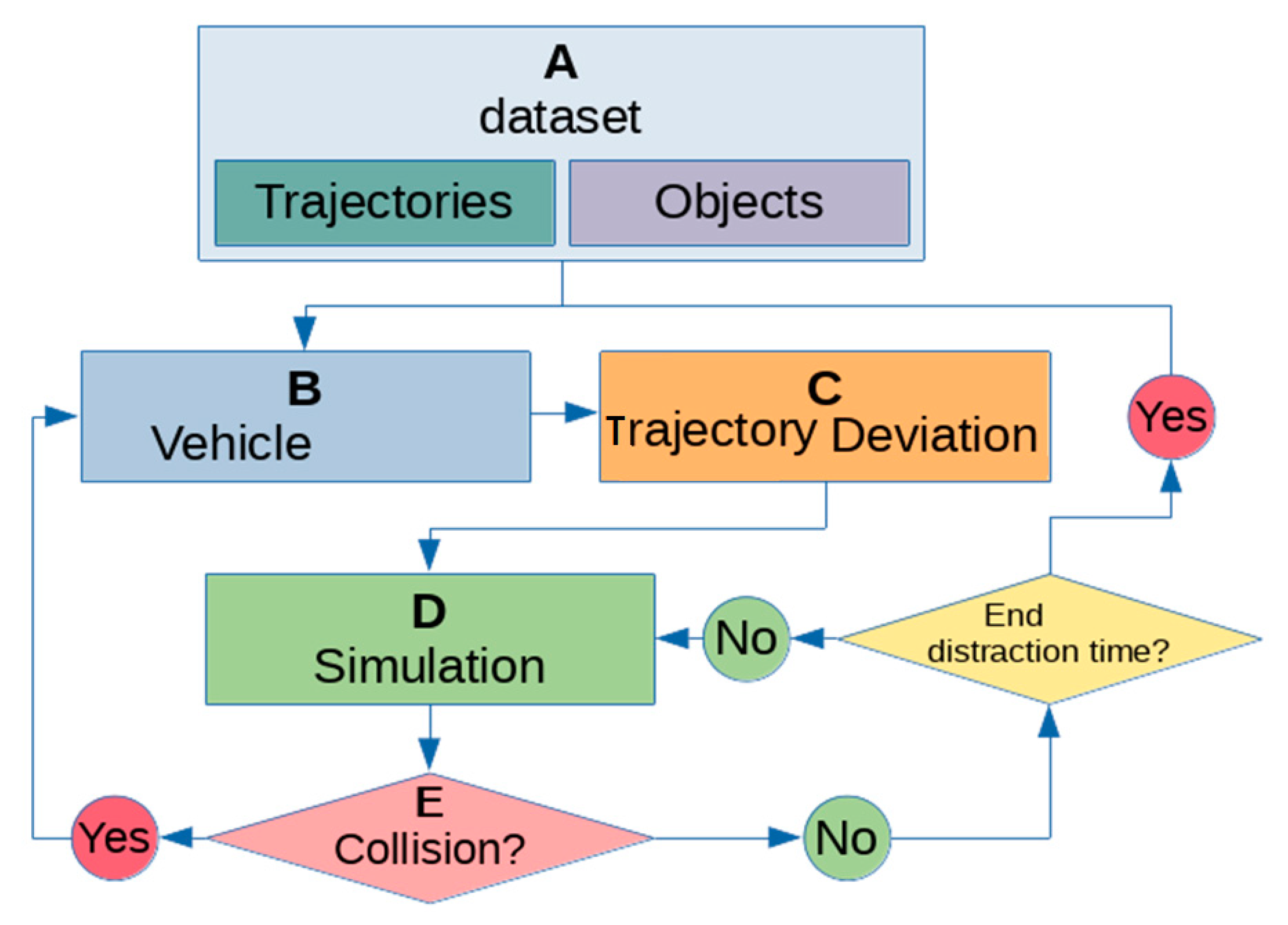
• This is the starting data set: The set of trajectories for a given time period in a defined traffic network in a road scenario.
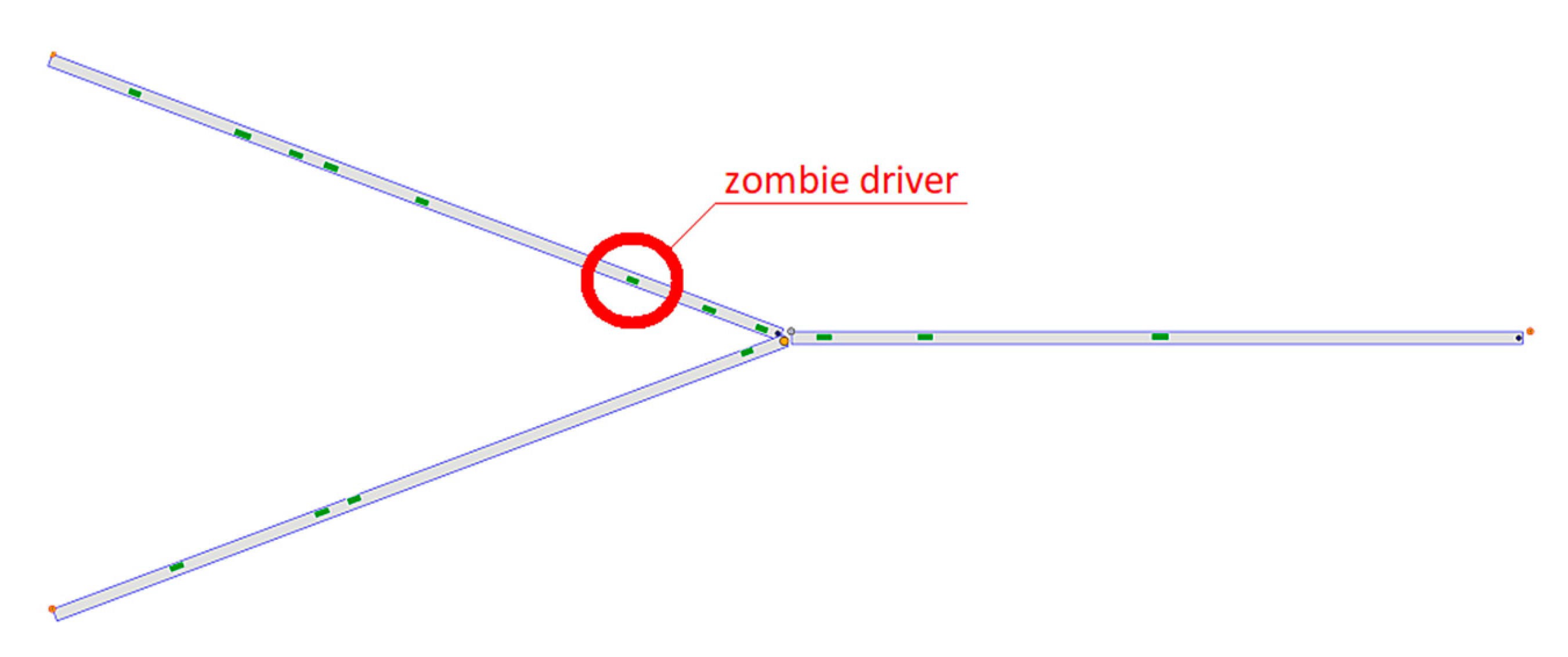
• Zombie (or bullet) vehicle choice: According to a random law (or deterministic procedure) a travelling vehicle position in a defined instant of time t is extracted from the traffic network; x being the chosen zombie vehicle (Figure 2) and p(x,t) the position at time t. The speed s(x,t) of vehicle x at time t is also known (as a bi-dimensional vector). All calculations in this paper are based on a deterministic procedure: Every vehicle is considered, every second of the simulation, for a deviated trajectory, and in this way a great number of potential crashes is generated.
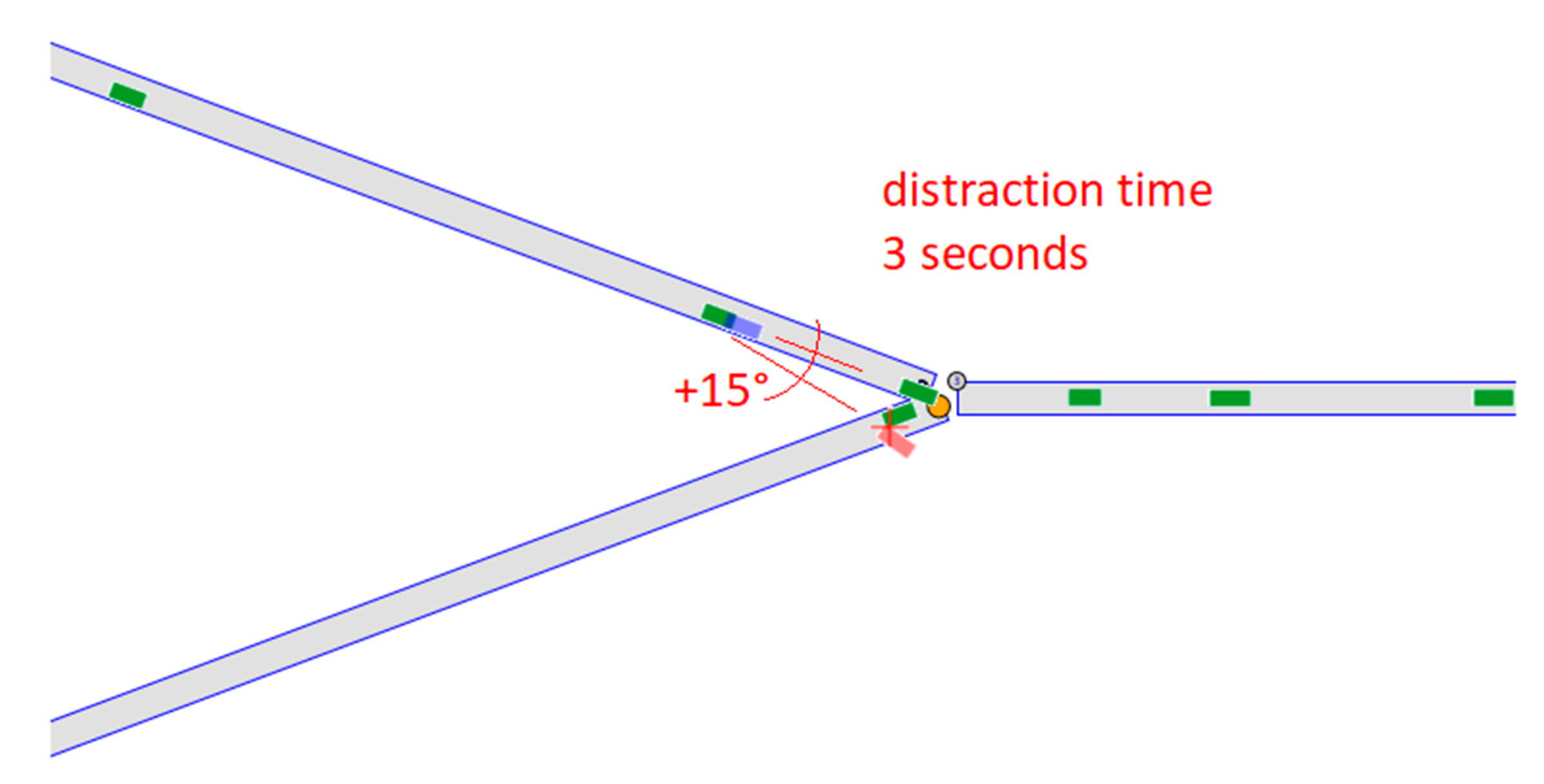
• Deviation of trajectory: The choice of a deviated trajectory in case of a driver error, driver distraction, or a mechanical failure is an open research field. With this model we would like to replicate all kinds of human mistakes a driver could possibly commit. This is not a simple task given the lack of an established probability distribution for driver mistakes. For this reason and in order to implement the first applications of our trajectory perturbation based model, we assumed a certain basic unsophisticated hypothesis, namely that the deviated trajectory follows a straight path at a constant speed which is equal to the speed of the vehicle before the deviation. The laws of momentum in physics suggest that this could be the more likely event in case the driver or the vehicle fails to perform in a normal way. Moreover, the application of a curved deviated trajectory corresponds to a straight trajectory at a certain (variable in time) angle. For this reason, an arrangement was contrived also to introduce the possibility of a certain angle between the deviated trajectory and the original correct trajectory.

In other words, given that the deviated trajectories can be generated into the Zombie Driver software according to any probabilistic law (or deterministic law) considering the initial correct position p(x,t) and speed s(x,t) of vehicle x at time t. We decided in the application reported in this paper to generate three perturbed trajectories (Figure 3) for each vehicle, with three different fixed angles corresponding to a straight trajectory and two deviated trajectories (+α) to the right and (−α) to the left.

The angle and the speed define the path of the deviated motion that is simulated for a given time of distraction (DT).

D.

Simulation of the deviated trajectory: With start at time t, the vehicle x is simulated as moving on the deviated trajectory for the next DT seconds.

E.

Potential collisions: When the deviated trajectory of a zombie vehicle brings the vehicle to collide with another vehicle (Figure 4) (it is important to note that in our first implementation all other vehicles are considered as moving on the original trajectories and cannot perform evasive maneuvers) or a road-side object, a potential collision is calculated by assessing the severity of the crash in terms of impact energy or with any other indicator.

The choice of a Y shaped intersection in Figure 2, Figure 3 and Figure 4 has been done just to depict some aspects of the methodology; the methodology applies to all kind of intersections and road traffic layouts.

The impact energy is calculated by applying the law of physics for inelastic collisions and considering individual vehicle parameters such as weight and geometric dimensions. Further details can be found in Astarita and Giofrè [5].

The general procedure repeats itself until an established number of zombie vehicles for consideration is reached, or when an established number of crashes are generated. This is one of the parameters of the methodology indicated in the following as Zombie Driver frequency.

This general procedure solves the four above-indicated issues. In fact:

• The methodology considers human error and can give a methodological explanation of why some kinds of crashes occurs in the field (e.g., single vehicle crashes which are not considered in classical surrogate safety performance indicators). The general assumption that “proximity” of vehicles is dangerous is maintained, and near-crash events are replaced with “potential crashes.”
• With the Zombie Driver software, the micro simulators can be used to evaluate the level of safety also in the presence of road-side objects. In this respect, in the procedure, the set of vehicle trajectories is required, and other additional information such as the location, geometrical shape, and elasticity coefficient of road-side objects and barriers.
• Since Zombie Driver explicitly simulates potential crashes, it is possible to evaluate the exact crash dynamic in terms of impact energy and the probability of having injuries and deaths.
• It allows one to consider conflicts between vehicles that are travelling on close dangerous trajectories that do not overlap.

Many parameters can be modified in the proposed methodology:

• The maximum distraction time: The time frame in which a driver is distracted and during which a collision with another vehicle or an obstacle may (or may not) occur. In our calculations we assumed deviated trajectories of 5 s.
• The distraction angle: The angle that will be given to two new lateral trajectories (considering that a third straight trajectory is always projected with an angle equal to 0 °). Currently this angle is set as a deterministic variable, but in the future it can be generated according to a Gaussian distribution with known mean and standard deviation.
• The minimum energy threshold: As a standard, this parameter is equal to zero in order to take into account all the collisions, but it is possible to modify it in order to consider only the more dangerous collisions that produce at least a fixed energy level.
• Size of the grid: One of the most useful outputs of Zombie Driver is the risk map. The risk maps are drawn by using a grid that is superimposed over the maps, and in which the risk areas are identified by using a chromatic scale. This parameter represents the size of the discretization of the study area, and therefore the mesh size of the grid. The standard size of the grid we have used in this work is 5 m (square cells). The calculation of intersection indicators has been performed by manually defining the intersection area with a set of square cells belonging to the 5 m defined grid.
• The zombie driver frequency: The frequency according to which a driver will commit a driving “error” moving on a deviated trajectory—in all calculations performed in this work, as already stated, we considered every vehicle, every second of the simulation as moving on three deviated trajectories.

The methodology is designed to return quick information and allow the user to understand what the critical points of the network are. Starting from regular safe trajectories it generates three deviated trajectories for every vehicle at every second in time. The result of repeating this methodology for every vehicle is a great number of potential crashes. For every potential crash the crash dynamic is perfectly known. With this information it is possible to extract many output parameters as described in the following:

• Collision energy means average energy (E_a), total energy (E_t), and maximum energy (E_m), detected from potential collisions on the network. It can be generated either by collisions between vehicles only or between vehicles and objects (e.g., trees, walls, etc.) and is divided into:
  General—Based on all the crashes detected on the road network under study.
  Single—For single vehicle, distinguished between the part of energy absorbed by the “zombie” vehicle carrying out the crash and the ones who suffer it. This is calculated also for single vehicle crashes and according to the collided object: Vehicle–vehicle collisions, vehicle–rigid objects, and vehicle–elastic objects.
• Difference between vehicle speed vectors (Delta-V), average (dV_a), total (dV_t), and maximum (dV_m). This represents the module of the vector difference between the two vehicles’ speed vectors during a collision.
• Index of collision severity, average (G_a), total (G_t), and maximum (G_m). This is the ratio between the energy that is generated during the collision and the time of distraction necessary for the event.
• Number of collisions, total (C_t) or per angle. These are the number of collisions that occurred during the analysis of the network, and they can also be differentiated according to the angle of the deviated trajectory.
• Distraction time, average (T_a) or per angle. This represents the average time that a “zombie” vehicle was driving on a deviated trajectory before being involved in a collision.

Since the Delta-V value for every vehicle involved in a potential crash is known, it is possible to estimate the probability of having a death or an injury for every vehicle involved in a potential crash. The formula used was proposed by Joksch in [80], and used by Evans in [81], and directly establishes a probability of death or injury as a function of Delta-V: $P={\left(\raisebox{1ex}{$∆V$}\!\left/ \!\raisebox{-1ex}{$\alpha $}\right.\right)}^k$, where $\alpha$ and k are two fixed parameters.

With this formula it is possible to calculate indicators for the potential number of deaths and injuries:

• Number of deaths, with (D_y) or without (D_n) safety belt. This is the sum of the probabilities of having or not having a dead person during a collision depending on the value of the difference between vehicle speed vectors.
• Number of injured, with (I_y) or without (I_n) safety belt. This is the sum of the probabilities of having or not having an injured person during a collision, depending on the value of the difference between vehicle speed vectors.

It must be noted that in this work we assumed a uniform distribution of errors among drivers, which is a simplification, since it would be possible to imagine a population of drivers with different characteristics and different potential errors. The model has the potential to explore changes in the driver population and the introduction of automatic vehicles by differentiating the potential errors among different vehicle categories. This is beyond the scope of this paper and represents a future promising development of our work, which might be worth investigating, once the necessary input data set is obtained.

The three main factors of traffic crashes are considered human factors, vehicle factors, and road environment factors. The classical safety performance analysis considers the first two factors by evidencing a risky situation when vehicles are driving close to each other in situations where a human error or a vehicle failure could lead to a crash. The Zombie Driver methodology also considers the road environment factor since a potential risky situation is also evidenced when a vehicle is driving near a dangerous road-side object. The Zombie Driver procedure in general can assess safety of a specific road-side design. In this paper this feature has not been applied since the road-side obstacles where not simulated in the Zombie Driver modelling.

3. Results

The crash data were extracted from the official reports of the urbane police of the city of Salerno, while traffic flows were computed by using video cameras placed at each intersection (for a greater in depth knowledge see El-Basyouny et al. [53]). In particular, four intersection scenarios (specified from I to IV) containing one or more single intersections (i = 1,…,9) were investigated: I (i = 1, 2, and 3), II (i = 4 and 5), III (i = 6, 7, and 8), and IV (i = 9). In

Table 1. Intersection scenarios and corresponding total crash data and total traffic volume ($\sum {\mathrm{VHP}}_{\mathrm{e},\mathrm{i}}$) during peak hours.

Intersection Scenario	Crash Data and Traffic Volume for Each Scenario	Time						Total Number of Crashes
		7:00–8:00 a.m.	8:00–9:00 a.m.	12:00 a.m.–1:00 p.m.	1:00–2:00 p.m.	6:00–7:00 p.m.	7:00–8:00 p.m.
I	Total number of crashes	1	8	25	13	5	4	56
(i = 1–3)	${\mathsf{\Sigma }\mathrm{VHP}}_{\mathrm{e},\mathrm{i}}$ (veh./h)	4539	6759	6620	6820	5878	5898
II	Total number of crashes	1	1	2	2	3	3	12
(i = 4 and 5)	${\mathsf{\Sigma }\mathrm{VHP}}_{\mathrm{e},\mathrm{i}}$ (veh./h)	5317	5902	4665	5150	5510	4982
III	Total number of crashes	1	4	3	4	5	5	22
(i = 6–8)	${\mathsf{\Sigma }\mathrm{VHP}}_{\mathrm{e},\mathrm{i}}$ (veh./h)	4974	7024	5248	4561	5583	4956
IV	Total number of crashes	0	4	0	3	2	1	10
(i = 9)	${\mathsf{\Sigma }\mathrm{VHP}}_{\mathrm{e},\mathrm{i}}$ (veh./h)	1310	2358	1998	2085	2046	1940
	Total number of crashes							100

are reported, during the peak hours, the corresponding crash data observed over a period of 5 years and entering traffic volumes VHP_e,i.

3.1. Micro-Simulation Calibration

The study scenarios were simulated through TRITONE. The supply and demand of the four areas in the various peak times has been modelled. Each scenario was calibrated using the information of the traffic flows available in the various road sections and the application of the GEH statistic. The GEH statistic was introduced by Geoffrey E. Havers in the 1970s and is an empirical formula that has proven useful for various traffic analysis purposes. In our case we apply the GEH statistic by comparing simulated flows with real measured flows:

$$\mathrm{GEH}=\sqrt{\frac{2{\left(Simulate-Real\right)}^2}{Simulate+Real}}<5.00$$

(2)

By applying this methodology in each section of the various simulated scenarios it was possible to establish that the GEH value was less than 5.0 in all the cases studied, and so the total success rate satisfies the standard requirement of having positive cases in more than 85% of the total cases, as indicated by the UK Highways Agency’s Design Manual for Roads and Bridges [82].

In all the simulations, Gipps’ car-following model was used and the flow was generated on the network with a negative exponential distribution between departures, while 30 random simulations were carried out for each scenario. The main output that TRITONE provided, in order to perform an analysis using the Zombie Driver methodology, was the set of vehicular trajectories. The exchanged data between TRITONE and Zombie Driver were not only the coordinates of the center of gravity of the vehicle, but also the four edges of the vehicle and the other vehicles’ specific parameters such as speed and mass.

3.2. Analysis of Simulation Results

The outcomes of simulation expressed in terms of the mean collision energy (E_a) and the number of collisions (C) evaluated by the Zombie Driver software are reported in

Table 2. Data description.

Intersection Scenario	Variables	Time
		7:00–8:00 a.m.	8:00–9:00 a.m.	12:00 a.m.–1:00 p.m.	1:00–2:00 p.m.	6:00–7:00 p.m.	7:00–8:00 p.m.
I	Mean Energy [kJ]	7.65	6.61	6.15	6.68	5.72	5.28
	Collisions	24,948	43,185	38,347	37,331	35,130	35,920
	Collisions *	6686	9088	9414	9093	8878	9321
II	Mean Energy [kJ]	119.65	76.29	52.30	132.43	60.04	90.88
	Collisions	10,283	17,290	22,456	7804	14,935	7896
	Collisions *	209	1492	1662	71	1070	86
III	Mean Energy [kJ]	57.05	54.90	62.31	57.63	51.95	47.68
	Collisions	37,236	80,828	42,809	31,533	47,904	39,918
	Collisions *	418	1450	1529	2310	796	757
IV	Mean Energy [kJ]	16.75	21.26	16.90	12.18	13.29	12.24
	Collisions	16,790	40,503	31,130	31,067	33,812	25,909
	Collisions *	3925	6718	5942	6139	5203	5421

* Collisions based on the safety indicators: Time to collision (TTC) and post-encroachment time (PET).

, together with the number of collisions (C*) calculated by using the TTC and PET as safety indicators. It must be noted that the collisions obtained with the Zombie Driver software are the (potential) crashes obtained by the perturbation of all the trajectories of all vehicles every second, while for TTC and PET the collisions are merely the violations of the threshold values of TTC and PET.

A summary statistic of the results is reported in

Table 3. Summary statistic of the results obtained by simulations.

	Intersection Scenario
	I			II			III			IV
	Mean Energy (kJ)	Collision *	Traffic Flow (veh./h)	Mean Energy (kJ)	Collision *	Traffic Flow (veh./h)	Mean Energy (kJ)	Collision *	Traffic Flow (veh./h)	Mean Energy (kJ)	Collision *	Traffic Flow (veh./h)
Mean	6.35	8746.67	6085.67	88.60	765.00	5254.33	55.25	1210.00	5391.00	15.44	5558.00	1956.17
SD	0.83	1027.16	865.87	32.17	731.84	429.22	5.04	688.95	869.02	3.55	963.55	348.05
Min	5.28	6686.00	4539.00	52.30	71.00	4665.00	47.68	418.00	4561.00	12.18	3925.00	1310.00
Max	7.65	9414.00	6820.00	132.43	1662.00	5902.00	62.31	2310.00	7024.00	21.26	6718.00	2358.00

* Collisions based on the safety indicators: TTC and PET.

.

4. Statistical Modelling

4.1. Literature Review on Random-Parameter Models

Given the simulation outputs, in terms of the safety indicators summarized in Table 3, we performed a statistical crash analysis, to establish the performance of each indicator in providing an estimation for the known number of real occurred crashes.

The potentiality of traditional statistical models and new ones has been discussed above all in [83,84,85]; as well as in [24,25,52] with reference to Italian studies. In the last decade, the random-parameter models, in which it is assumed that the regression parameters are random, have been more and more adopted to take into account the unobserved heterogeneity; which is associated with the variables (covariates). In this respect, several studies show the advantages of random-parameter models compared to the fixed-parameter ones in terms of goodness-of-fit [26,86,87,88,89]. However, it is to be noted that in the aforementioned studies the random parameters are assumed to be independent of each other. According to Conway and Kniesner [90], instead, when the correlations between the random parameters are neglected, the estimates may be biased.

The correlated random-parameter models have still been little investigated in the literature. Some studies can be found in Conway et al. [91] that employed a correlated random-parameter Tobit model, showing a better goodness-of-fit compared to the corresponding uncorrelated random-parameter model. Coruh et al. [92] found that the correlated random-parameter negative binomial (NB) model was statistically superior to the corresponding uncorrelated random-parameter NB model. Hou et al. [93] also found that the correlated random-parameter NB model is more appropriate. By investigating the crash frequency in Italian tunnels, Caliendo et al. [18] developed a univariate correlated random-parameter model, which is better in terms of goodness-of-fit if compared both to the uncorrelated random-parameter model and the random-intercept one (the latter is also known as random-effect model; for a more in-depth knowledge see Greene [94] and Hilbe [95]. Finally, Saeed et al. [96] found that the correlations among the random parameters were statistically significant.

In light of the above considerations, given the aforementioned lacuna of studies, in this paper we apply a correlated random-parameters model for the statistical analysis of crashes that occurred at the four intersections scenarios investigated.

4.2. Methodology

In crash analysis, it is typically assumed that the fluctuation of crash counts, say $Y_i$, which occurs at the peak hour time i of the investigated intersection scenarios during the 5-year monitoring period, is a negative binomial (NB) distribution [53]. However, since we found from a preliminary statistical analysis that $\alpha$ (over-dispersion parameter of the NB model) converged to zero, a univariate correlated random-parameter Poisson (CRPP) model was used in the present paper. Therefore, Y_i is distributed as follows:

$$Y_i ~ Poisson \left({\lambda }_i\right).$$

(3)

Let λ_i and X denote the expectation of Y_i and the vector of k covariates, respectively. For λ_i, the following log-linear function is used:

$${\lambda }_i=exp\left({\mathit{X}}_{\mathit{i}}^{\mathit{T}}{\mathit{\beta }}_{\mathit{i}}\right);$$

(4)

where β_i is the vector of random-parameters for observation i, which assumes a multivariate normal distribution written as follows:

$${\mathit{\beta }}_{\mathit{i}}=\mathit{b}+\mathit{C}{\mathit{\omega }}_{\mathit{i}};$$

(5)

where b is the mean vector; C is the variance-covariance matrix, which allows one to take into account the correlations among the elements of β_i; and ω_i is the randomly and independently distributed uncorrelated vector term. In particular, b and C are defined as follows:

$$\mathit{b}=\left[\begin{array}{c}{\beta }_1\\ {\beta }_2\\ \dots \\ {\beta }_{j-1}\\ {\beta }_j\end{array}\right] and \mathit{C}=\left[\begin{array}{ccccc}{\left({\sigma }_1\right)}^2& {\sigma }_{1,2}& \dots & {\sigma }_{1,j-1}& {\sigma }_{1,j}\\ {\sigma }_{2,1}& {\left({\sigma }_2\right)}^2& \dots & {\sigma }_{2,j-2}& {\sigma }_{2,j}\\ \dots & \dots & \dots & \dots & \dots \\ {\sigma }_{j-1,1}& {\sigma }_{j-1,2}& \dots & {\left({\sigma }_{j-1}\right)}^2& {\sigma }_{j-1,j}\\ {\sigma }_{j,1}& {\sigma }_{j,2}& \dots & {\sigma }_{j,j-1}& {\left({\sigma }_j\right)}^2\end{array}\right];$$

(6)

in which j is the number of random parameters. Clearly, in an uncorrelated random-parameter model, the off-diagonal elements in the variance-covariance matrix are equal to zero.

In the present paper, we investigate and compare two different CRPP models, which include different sets of covariates: (i) Model A establishes a relationship between: Collisions (C) calculated in simulation on the basis of the safety indicators such as the TTC and PET, traffic flow (TF, indicated in the text also as VHP_e;i), and dummy variable (Du) for accounting for the occurrence of a much higher number of crashes at the Scenario I in the afternoon peak hours (between 12:00 a.m. and 1:00 p.m., and between 1:00 p.m. and 2:00 p.m.); (ii) Model B involves the following explanatory variables: Mean energy (E_a), traffic flow (TF), and dummy variable (Du). Note that the Du assumes a value of 1 with reference to the afternoon peak hours of the Scenario I and 0 elsewhere.

In each model, the maximization procedure of the likelihood function is employed for estimating the parameters of the model, while a method based on 2000 Halton draws (see in detail Saeed et al. [97]) is adopted to obtain an efficient convergence for the numerical integration in the estimate.

4.3. Procedure for Choosing the Statistically More Significant Variables and Models’ Comparison

In order to identify the subset of explanatory variables the effect of which is not negligible on crash counts, a procedure based on the likelihood ratio test (LRT) is adopted. The LRT statistic, which in our case has an asymptotic chi-square distribution (${\chi }^2$) with 1 degree of freedom, is defined as follows:

$$\mathsf{\Lambda }=2\left[l\left(\widehat{\mathit{\beta }},\widehat{\phi }\right)-l\left(\widehat{{\mathit{\beta }}^{\prime }},{\beta }_k=0,\widehat{\phi }\right)\right],$$

(7)

where $l\left(\widehat{\mathit{\beta }},\widehat{\phi }\right)$ is the log-likelihood of the regression model containing all covariates; and $l\left(\widehat{{\mathit{\beta }}^{\prime }},{\beta }_k=0,\widehat{\phi }\right)$ is the log-likelihood of the regression model with the covariate $k$ out. Since a significance level of 10% is assumed in this paper, a variable is included in the regression model when the LRT statistic corresponding to the model without the same is at least 2.71.

With the purpose of comparing Models A and B in terms of goodness-of-fit, also the root mean square error (RMSE) is used. In general, models with lower RMSE are preferred:

$$RMSE=\sqrt{\frac{1}{n}{{\displaystyle \sum }}_i{\left(Y_i-{\lambda }_i\right)}^2},$$

(8)

in which $Y_i$ is the crash associated with observation i; λ_i denotes the expectation of $Y_i$; and n is the sample size.

5. Discussion and Analysis of Results

Table 4. Model A—Estimated results of the correlated random-parameter Poisson (CRPP) model.

Variables	Model A—Correlated Random-Parameter Poisson (CRPP) Model
	Point Estimate	Standard Error	Likelihood Ratio Test (LRT) Statistic
Fixed Parameters
Constant	−0.385	0.577
C* (Collisions)/10.000	0.624	0.513	2.99
Random Parameters
TF (Traffic Flow)/10.000 (veh./h)	2.468	1.044	9.39
Du (Dummy variable)	1.067	0.477	8.31
Other statistical information
Number of observations	24
Log likelihood function	−45.328

C* (Collisions based on the safety indicators: TTC and PET).

and

Table 5. Model B—Estimated results of the correlated random-parameter Poisson (CRPP) model.

Variables	Model B—Correlated Random-Parameter Poisson (CRPP) Model
	Point Estimate	Standard Error	LRT Statistic
Fixed Parameters
Constant	0.029	0.455
Random Parameters
Ea (Mean Energy) (J × 104)	−0.071	0.061	3.66
TF (Traffic Flow)/10.000 (veh./h)	2.737	1.057	11.16
Du (Dummy variable)	1.094	0.427	7.90
Other statistical information
Number of observations	24
Log likelihood function	−44.991

show the estimations results provided by Models A and B, respectively.

From Table 4 it is possible to observe that the expected number of crashes increases in a non-linear way with: The collisions (C*), traffic flow (TF), and dummy variable (Du). For Model B (Table 5), instead, one may note that the expected number of crashes is negatively associated with the mean energy (E_a) and positively with other variables (i.e., traffic flow (TF), and dummy variable (Du)). In both models, the LRT statistic associated with each variable is at least 2.71. This means that all covariates are statistically significant at a level less than 10%.

However, given the values of the log likelihood function, Model B is statistically equivalent to Model A.

Since the negative sign associated with the covariate E_a (in Model B) does not appear to have a logical explanation, in order to get a better understanding of the effects of the E_a on the crashes, according to the authors the correlation coefficients matrix of random parameters should be more especially commented on.

Table 6. Model A—Correlation coefficients matrix of parameters.

Variables	TF	Du
TF (Traffic Flow)/10.000	1.00	0.19
Du (Dummy variable)	0.19	1.00

and

Table 7. Model B—Correlation coefficients matrix of parameters.

Variables	Ea	TF	Du
Ea (Mean Energy)	1.00	0.11	−0.36
TF (Traffic Flow)/10.000	0.11	1.00	0.88
Du (Dummy variable)	−0.36	0.88	1.00

report the correlation coefficients matrix of random-parameters for Model A and Model B, respectively.

In particular, Table 7 shows that the mean energy (E_a) is positively correlated with the traffic flow (TF) (i.e., correlation coefficient = +0.11). This means that an increase of the E_a makes the effect of traffic flow more significant on increasing crashes.

Regarding the comparison between Models A and B in terms of-goodness-of-fit, this was carried out in terms of the RMSE. From

Table 8. Model (s’) comparison by root mean square error (RMSE) (Models A and B).

Intersection Scenario	Number of Total Crashes (5 Years)	Model A		Model B
		Expected Number of Total Crashes (5 Years)	RMSE	Expected Number of Total Crashes (5 Years)	RMSE
I	56.00	56.79	3.83	56.48	3.96
II	12.00	15.76	1.16	14.23	1.00
III	22.00	17.02	1.63	18.73	1.51
IV	10.00	9.44	1.35	9.49	1.40
TOT	100.00	99.00	2.26	98.94	2.29

one can see that the estimated number of crashes is quite similar for both models, as well as their being almost equal to the number of real crashes observed in the field.

Summing up, Models A and B and are statistically equivalent both in terms of log likelihood function and RMSE. The total number of crashes in 5 years estimated by the aforementioned models are also similar to each other. Moreover, the total number of estimated crashes is almost equal to that measured in the field over the same period of time. Therefore, the results appear to justify the use of the mean energy (E_a), in alternative to the number of collisions (C*), as a surrogate safety measure.

6. Summary and Conclusions

This research was motivated by the need to explore the potentiality of the proposed methodology for assessing safety at urban intersections using the collision energy as a surrogate safety measures in alternative to the number of collisions based on (the) TTC and PET.

The results show that the statistical model (Model B), in which the mean energy (E_a) is present, is statistically equivalent to the model based on collisions (Model A), and that it estimates the same number of crashes observed in the field.

The statistical analysis applied in Chapter 6 that is performed with state of the art statistical modelling shows, with the coefficient correlation matrix, that the E_a makes the effect of traffic flow on increasing crashes more significant, in contrast with the negative sign of the estimation point.

In conclusion, we can affirm that this methodology can allow engineers to quickly individualize the critical points of a road network by using simulated vehicular trajectories and the collision energy as a surrogate safety indicator.

The proposed Zombie Driver methodology depends on many parameters that should be properly calibrated. It would be logical to calibrate our methodology according to a rich set of traffic networks where crash data and traffic data are both available. These calibration efforts fall outside the scope of this paper and can be investigated in future research.

This study was carried on in a geographically limited area: Some intersections in the urban network of Salerno. Many parameters and model characteristics were set at default values instead of performing an accurate calibration on a limited data set. The TTC and PET analyses carried out in this paper are also based on many parameters that assume default values. In fact, the original default values adopted in the SSAM software have not been obtained with a real calibration on an extensive set of traffic and crash data.

However, for a more consolidated verification of the methodology proposed a more extended data set (possibly created with more numerous intersections of different cities) could become the base to obtain more general and more reliable results. Therefore, further research and data gathering will help to establish which safety indicator offers the more accurate crash estimations.

The proposed Zombie Driver methodology might also be usefully applied on mixed traffic scenarios with traditional and autonomous vehicles, once accurate information on the specification and development of autonomous vehicles is available. In other words, given the calibrated error frequency of both autonomous vehicles and human driven vehicles, the Zombie Driver procedure could be useful to evaluate the safety of different road traffic layouts. Information on autonomous vehicles could be obtained from traffic sequence charts [98] that could provide “a concise, intuitive specification language for capturing expected and forbidden behaviors of autonomous vehicles in the space of all possible traffic situations.”

It must be noted that while some of the observed crashes during the 5 years may be caused by adverse weather and poor road surface conditions, our database did not include this information. When one or more variables are omitted in a database of crashes, the so-called “unobserved heterogeneity” phenomenon across data might occur. However, according to the international literature, the unobserved heterogeneity may be captured by using the so-called random-parameter models in the statistical analysis of crashes. This is the case of our study, in which a statistical analysis based on random-parameter modes is used (for a more in depth knowledge, please see Milton et al. [87]); in this sense, our approach (and also the classic SSAM indicators) considers (indirectly) weather and road surface conditions risks. This is because the occurrence of deviated trajectory could originate from these adverse conditions, and a vehicle crash which is in general due to this kind of adverse condition would more likely occur where there is exposure in terms of traffic flows or out-of-scale safety indicators. The reproduction of the 8760 yearly hours of traffic with traffic simulation is possible, given enough traffic and weather data, and is one among the several possible future developments of the topics discussed in this research.

References

- Marzano, V.; Tocchi, D.; Papola, A.; Aponte, D.; Simonelli, F.; Cascetta, E. Incentives to freight railway undertakings compensating for infrastructural gaps: Methodology and practical application to Italy. Transp. Res. Part A Policy Pract. 2018. [Google Scholar] [CrossRef]
- Astarita, V.; Florian, M.; Musolino, G. A microscopic traffic simulation model for the evaluation of toll station systems. In Proceedings of the IEEE Conference on Intelligent Transportation Systems, Oakland, CA, USA, 25–29 August 2001. [Google Scholar]
- Astarita, V.; Giofré, V.; Guido, G.; Vitale, A. Investigating road safety issues through a microsimulation model. Procedia -Soc. Behav. Sci. 2011, 20, 226–235. [Google Scholar] [CrossRef] [Green Version]
- Young, W.; Sobhani, A.; Lenné, M.G.; Sarvi, M. Simulation of safety: A review of the state of the art in road safety simulation modelling. Accid. Anal. Prev. 2014. [Google Scholar] [CrossRef] [PubMed]
- Astarita, V.; Giofré, V.P. From traffic conflict simulation to traffic crash simulation: Introducing traffic safety indicators based on the explicit simulation of potential driver errors. Simul. Model. Pr. Theory 2019, 94, 215–236. [Google Scholar] [CrossRef]
- Osorio, C.; Punzo, V. Efficient calibration of microscopic car-following models for large-scale stochastic network simulators. Transp. Res. Part B Methodol. 2019. [Google Scholar] [CrossRef]
- Martinez, F.J.; Toh, C.K.; Cano, J.C.; Calafate, C.T.; Manzoni, P. A survey and comparative study of simulators for vehicular ad hoc networks (VANETs). Wirel. Commun. Mob. Comput. 2011. [Google Scholar] [CrossRef]
- Gentile, G. New formulations of the stochastic user equilibrium with logit route choice as an extension of the deterministic model. Transp. Sci. 2018. [Google Scholar] [CrossRef]
- Cantarella, G.E.; Di Febbraro, A.; Di Gangi, M.; Giannattasio, O. Stochastic Multi-Vehicle Assignment to Urban Transportation Networks. In Proceedings of the MT-ITS 2019—6th International Conference on Models and Technologies for Intelligent Transportation Systems, Cracow, Poland, 5–7 June 2019. [Google Scholar]
- Cantarella, G.E.; Watling, D.P. A general stochastic process for day-to-day dynamic traffic assignment: Formulation, asymptotic behaviour, and stability analysis. Transp. Res. Part B Methodol. 2016. [Google Scholar] [CrossRef]
- Trozzi, V.; Gentile, G.; Kaparias, I.; Bell, M.G.H. Effects of Countdown Displays in Public Transport Route Choice Under Severe Overcrowding. Networks Spat. Econ. 2015. [Google Scholar] [CrossRef] [Green Version]
- Kucharski, R.; Gentile, G. Simulation of rerouting phenomena in Dynamic Traffic Assignment with the Information Comply Model. Transp. Res. Part B Methodol. 2018. [Google Scholar] [CrossRef]
- Marzano, V.; Papola, A.; Simonelli, F.; Papageorgiou, M. A Kalman Filter for Quasi-Dynamic o-d Flow Estimation/Updating. IEEE Trans. Intell. Transp. Syst. 2018. [Google Scholar] [CrossRef]
- Papola, A.; Tinessa, F.; Marzano, V. Application of the Combination of Random Utility Models (CoRUM) to route choice. Transp. Res. Part B Methodol. 2018. [Google Scholar] [CrossRef]
- Papola, A. A new random utility model with flexible correlation pattern and closed-form covariance expression: The CoRUM. Transp. Res. Part B Methodol. 2016. [Google Scholar] [CrossRef]
- Hauer, E. On the estimation of the expected number of accidents. Accid. Anal. Prev. 1986. [Google Scholar] [CrossRef]
- Miaou, S.P.; Lum, H. Modeling vehicle accidents and highway geometric design relationships. Accid. Anal. Prev. 1993. [Google Scholar] [CrossRef]
- Caliendo, C.; De Guglielmo, M.L.; Russo, I. Analysis of crash frequency in motorway tunnels based on a correlated random-parameters approach. Tunn. Undergr. Space Technol. 2019. [Google Scholar] [CrossRef]
- Miaou, S.P. The relationship between truck accidents and geometric design of road sections: Poisson versus negative binomial regressions. Accid. Anal. Prev. 1994. [Google Scholar] [CrossRef] [Green Version]
- Shankar, V.; Mannering, F.; Barfield, W. Effect of roadway geometrics and environmental factors on rural freeway accident frequencies. Accid. Anal. Prev. 1995. [Google Scholar] [CrossRef]
- Hauer, E. Observational before—After Studies in Road Safety: Estimating the Effect of Highway and Traffic Engineering Measures on Road Safety; Pergamon: Bergama, Turkey, 1997; ISBN 9780080430539. [Google Scholar]
- Abdel-Aty, M.A.; Radwan, A.E. Modeling traffic accident occurrence and involvement. Accid. Anal. Prev. 2000. [Google Scholar] [CrossRef]
- Yan, X.; Radwan, E.; Abdel-Aty, M. Characteristics of rear-end accidents at signalized intersections using multiple logistic regression model. Accid. Anal. Prev. 2005, 37, 983–995. [Google Scholar] [CrossRef] [PubMed]
- Caliendo, C.; Guida, M.; Parisi, A. A crash-prediction model for multilane roads. Accid. Anal. Prev. 2007. [Google Scholar] [CrossRef] [PubMed]
- Caliendo, C.; Guida, M. A New Bivariate Regression Model for the Simultaneous Analysis of Total and Severe Crashes Occurrence. J. Transp. Saf. Secur. 2014. [Google Scholar] [CrossRef]
- Caliendo, C.; De Guglielmo, M.L.; Guida, M. Comparison and analysis of road tunnel traffic accident frequencies and rates using random-parameter models. J. Transp. Saf. Secur. 2016. [Google Scholar] [CrossRef]
- Hydén, C.; Linderhonm, L. The Swedish Traffic Conflicts Technique. In International Calibration Study of Traffic Conflict Techniques; Asmussen, E., Ed.; Springer Science & Business Media: Berlin, Germany, 2012. [Google Scholar]
- Hyden, C. The Development of a Method for Traffic Safety Evaluation: The Swedish Traffic Conflicts Technique. Ph.D. Thesis, Lund Institute of Technology, Lund, Sweden, 1987. [Google Scholar]
- Perkins, S.R.; Harris, J.L. Traffic conflict characteristics-accident potential at intersections. In Traffic Safety and Accident Research -Highway Research Record 225; Highway Research Board: Washington, DC, USA, 1968. [Google Scholar]
- Baker, W.T. An evaluation of the traffic conflicts technique. Highw. Res. Rec. 1972, 384, 1–8. [Google Scholar]
- Oh, C.; Kim, T. Estimation of rear-end crash potential using vehicle trajectory data. Accid. Anal. Prev. 2010. [Google Scholar] [CrossRef]
- Guido, G.; Vitale, A.; Gallelli, V.; Figliomeni, G. Level of Safety on Two-Lane Undivided Rural Highways; Trans Tech Publications Ltd.: Stafa-Zurich, Switzerland, 2013; Volume 253, ISBN 9783037855645. [Google Scholar]
- Gettman, D.; Head, L. Surrogate Safety Measures from Traffic Simulation Models. Transp. Res. Rec. J. Traportation Res. Board 2003. [Google Scholar] [CrossRef] [Green Version]
- Saccomanno, F.; Cunto, F.; Guido, G.; Vitale, A. Comparing Safety at Signalized Intersections and Roundabouts Using Simulated Rear-End Conflicts. Transp. Res. Rec. J. Transp. Res. Board 2008. [Google Scholar] [CrossRef]
- Astarita, V.; Guido, G.; Vitale, A.; Giofré, V. A new microsimulation model for the evaluation of traffic safety performances. Eur. Transp. -Trasp. Eur. 2012, 51, 1–2. [Google Scholar]
- Kim, H.; Kim, Y.; Jang, K. Systematic Relation of Estimated Travel Speed and Actual Travel Speed. IEEE Trans. Intell. Transp. Syst. 2017. [Google Scholar] [CrossRef]
- Hayward, J. Near Misses as a Measure of Safety at Urban Intersections. Ph.D. Thesis, Department of Civil Engineering, Pennsylvania State University, Pennsylvania, PA, USA, 1971. [Google Scholar]
- Minderhoud, M.M.; Bovy, P.H.L. Extended time-to-collision measures for road traffic safety assessment. Accid. Anal. Prev. 2001. [Google Scholar] [CrossRef]
- Huguenin, F.; Torday, A.; Dumont, A. Evaluation of traffic safety using microsimulation. In Proceedings of the 5th Swiss Transport Research Conference, Ascona, Switzerland, 9–11 March 2005. [Google Scholar]
- Allen, B.L.; Shin, B.T.; Cooper, P. Analysis of traffic conflicts and collisions. Transp. Res. Rec. 1978, 667, 67–74. [Google Scholar]
- Caliendo, C. Delay time model at unsignalized intersections. J. Transp. Eng. 2014. [Google Scholar] [CrossRef]
- Caliendo, C.; De Guglielmo, M.L. Road transition zones between the rural and urban environment: Evaluation of speed and traffic performance using a microsimulation approach. J. Transp. Eng. 2013. [Google Scholar] [CrossRef]
- Guido, G.; Astarita, V.; Giofré, V.; Vitale, A. Safety performance measures: A comparison between microsimulation and observational data. Procedia -Soc. Behav. Sci. 2011, 20, 217–225. [Google Scholar] [CrossRef] [Green Version]
- Astarita, V.; Giofrè, V.; Guido, G.; Vitale, A.; Festa, D.; Vaiana, R.; Iuele, T.; Mongelli, D.; Rogano, D.; Gallelli, V. New features of Tritone for the evaluation of traffic safety performances. In Transport Infrastructure and Systems; Taylor & Francis Group: London, UK, 2017; pp. 625–632. [Google Scholar]
- Darzentas, J.; Cooper, D.F.; Storr, P.A.; Mcdowell, M.R.C. Simulation of road traffic conflicts at T-junctions. Simulation 1980. [Google Scholar] [CrossRef]
- Cunto, F.J.C.; Saccomanno, F.F. Microlevel Traffic Simulation Method for Assessing Crash Potential at Intersections. In Proceedings of the Transportation Research Board 86th Annual Meeting, Washington, DC, USA, 21–23 January 2007. [Google Scholar]
- Cunto, F.; Saccomanno, F.F. Calibration and validation of simulated vehicle safety performance at signalized intersections. Accid. Anal. Prev. 2008. [Google Scholar] [CrossRef]
- Yang, H.; Ozbay, K.; Bartin, B. Application of Simulation-Based Traffic Conflict Analysis for Highway Safety Evaluation. In Proceedings of the 12th World Conference on Transport Research, Lisbon, Portugal, 11–15 July 2010. [Google Scholar]
- Wang, C.; Stamatiadis, N. Evaluation of a simulation-based surrogate safety metric. Accid. Anal. Prev. 2014. [Google Scholar] [CrossRef]
- Gettmann, D.; Pu, L.; Sayed, T.; Shelby, S. Surrogate Safety Assessment Model and Validation: Final Report; United States. Federal Highway Administration. Office of Safety Research and Development: McLean, VA, USA, 2008.
- Dijkstra, A.; Marchesini, P.; Bijleveld, F.; Kars, V.; Drolenga, H.; van Maarseveen, M. Do Calculated Conflicts in Microsimulation Model Predict Number of Crashes? Transp. Res. Rec. J. Transp. Res. Board 2010. [Google Scholar] [CrossRef]
- Caliendo, C.; Guida, M. Microsimulation Approach for Predicting Crashes at Unsignalized Intersections Using Traffic Conflicts. J. Transp. Eng. 2012. [Google Scholar] [CrossRef]
- El-Basyouny, K.; Sayed, T. Safety performance functions using traffic conflicts. Saf. Sci. 2013. [Google Scholar] [CrossRef]
- Huang, F.; Liu, P.; Yu, H.; Wang, W. Identifying if VISSIM simulation model and SSAM provide reasonable estimates for field measured traffic conflicts at signalized intersections. Accid. Anal. Prev. 2013. [Google Scholar] [CrossRef] [PubMed]
- Zhou, H.; Huang, F. Development of Traffic Safety Evaluation Method based on Simulated Conflicts at Signalized Intersections. Procedia-Soc. Behav. Sci. 2013. [Google Scholar] [CrossRef] [Green Version]
- Ambros, J.; Turek, R.; Paukrt, J. Road safety evaluation using traffic conflicts: Pilot comparison of micro-simulation and observation. In Proceedings of the International Conference on Traffic and Transport Engineering, Belgrade, Serbia, 27–28 November 2014. [Google Scholar]
- Shahdah, U.; Saccomanno, F.; Persaud, B. Integrated traffic conflict model for estimating crash modification factors. Accid. Anal. Prev. 2014. [Google Scholar] [CrossRef] [PubMed]
- Shahdah, U.; Saccomanno, F.; Persaud, B. Application of traffic microsimulation for evaluating safety performance of urban signalized intersections. Transp. Res. Part C Emerg. Technol. 2015. [Google Scholar] [CrossRef]
- Zha, L.; Songchitruksa, P.; Balke, K. Next Generation Safety Performance Monitoring at Signalized Intersections Using Connected Vehicle Technology. Master’s Thesis, Texas A & M University, College Station, TX, USA, 2014. [Google Scholar]
- Morando, M.M.; Tian, Q.; Truong, L.T.; Vu, H.L. Studying the Safety Impact of Autonomous Vehicles Using Simulation-Based Surrogate Safety Measures. J. Adv. Transp. 2018. [Google Scholar] [CrossRef]
- Astarita, V.; Festa, D.C.; Giofrè, V.P.; Guido, G.; Vitale, A. The use of Smartphones to assess the Feasibility of a Cooperative Intelligent Transportation Safety System based on Surrogate Measures of Safety. Procedia Comput. Sci. 2018, 134, 427–432. [Google Scholar] [CrossRef]
- Vaiana, R.; Iuele, T.; Astarita, V.; Caruso, M.V.; Tassitani, A.; Zaffino, C.; Giofrè, V.P. Driving behavior and traffic safety: An acceleration-based safety evaluation procedure for smartphones. Mod. Appl. Sci. 2014. [Google Scholar] [CrossRef]
- Astarita, V.; Guido, G.; Vitale, A.; Gallelli, V. Analysis of Non-Conventional Roundabouts Performances Through Microscopic Traffic Simulation. Appl. Mech. Mater. 2014. [Google Scholar] [CrossRef]
- Astarita, V. Flow propagation description in dynamic network loading models. In Proceedings of the International Conference on Applications of Advanced Technologies in Transportation Engineering, Capri, Italy, 31 July 1996. [Google Scholar]
- Guido, G.; Saccomanno, F.; Vitale, A.; Astarita, V.; Festa, D. Comparing safety performance measures obtained from video capture data. J. Transp. Eng. 2011, 137. [Google Scholar] [CrossRef]
- Guido, G.; Vitale, A.; Saccomanno, F.F.; Festa, D.C.; Astarita, V.; Rogano, D.; Gallelli, V. Using Smartphones as a Tool to Capture Road Traffic Attributes. Appl. Mech. Mater. 2013. [Google Scholar] [CrossRef]
- Astarita, V.; Guido, G.; Mongelli, D.; Giofrè, V.P. A co-operative methodology to estimate car fuel consumption by using smartphone sensors. Transport 2015, 30. [Google Scholar] [CrossRef] [Green Version]
- Festa, D.C.; Mongelli, D.W.E.; Astarita, V.; Giorgi, P. First results of a new methodology for the identification of road surface anomalies. In Proceedings of the 2013 IEEE International Conference on Service Operations and Logistics, and Informatics, Dongguan, China, 28–30 July 2013. [Google Scholar]
- Astarita, V.; Guido, G.; Mongelli, D.W.E.; Giofrè, V.P. Ecosmart and TutorDrive: Tools for fuel consumption reduction. In Proceedings of the 2014 IEEE International Conference on Service Operations and Logistics, and Informatics, SOLI 2014, Qingdao, China, 8–10 October 2014. [Google Scholar]
- Astarita, V.; Giofrè, V.P. Trajectory Perturbation in Surrogate Safety Indicators. Transp. Res. Procedia 2020, 8. [Google Scholar] [CrossRef]
- Davis, G.A.; Hourdos, J.; Xiong, H.; Chatterjee, I. Outline for a causal model of traffic conflicts and crashes. Accid. Anal. Prev. 2011. [Google Scholar] [CrossRef] [PubMed]
- Bevrani, K.; Chung, E. An Examination of the Microscopic Simulation Models to Identify Traffic Safety Indicators. Int. J. Intell. Transp. Syst. Res. 2012. [Google Scholar] [CrossRef] [Green Version]
- Stutts, J.; Gish, K. Distraction in Everyday Driving. Rep. Prep. AAA Found. Trafic Saf. 2003. [Google Scholar] [CrossRef] [Green Version]
- Pu, L.; Joshi, R. Surrogate Safety Assessment Model (SSAM): Software User Manual. 2008. Available online: https://rosap.ntl.bts.gov/view/dot/1008 (accessed on 26 August 2020).
- Souleyrette, R.; Hochstein, J. Development of a Conflict Analysis Methodology Using SSAM. 2012. Available online: https://works.bepress.com/reginald_souleyrette/45/ (accessed on 26 August 2020).
- Ivan, J.N.; Konduri, K.C. Chapter 15. Crash Severity Methods. In Safe Mobility: Challenges, Methodology and Solutions (Transport and Sustainability, Vol. 11); Dominique, L., Washington, S., Eds.; Emerald Publishing Limited: Bingley, UK, 2018; pp. 325–350. [Google Scholar]
- Laureshyn, A.; De Ceunynck, T.; Karlsson, C.; Svensson, Å.; Daniels, S. In search of the severity dimension of traffic events: Extended Delta-V as a traffic conflict indicator. Accid. Anal. Prev. 2017. [Google Scholar] [CrossRef] [Green Version]
- Guido, G.; Astarita, V.; Giofré, V.P.; Vitale, A. Using traffic microsimulation to evaluate potential crashes: Some results. In Proceedings of the 2019 IEEE/ACM 23rd International Symposium on Distributed Simulation and Real Time Applications (DS-RT), Rende, Italy, 7–9 October 2019. [Google Scholar]
- Alonso, B.; Astarita, V.; Dell’Olio, L.; Giofrè, V.P.; Guido, G.; Marino, M.; Sommario, W.; Vitale, A. Validation of Simulated Safety Indicators with Traffic Crash Data. Sustainability 2020, 12, 925. [Google Scholar] [CrossRef] [Green Version]
- Joksch, H.C. Velocity change and fatality risk in a crash—A rule of thumb. Accid. Anal. Prev. 1993. [Google Scholar] [CrossRef]
- Evans, L. Driver injury and fatality risk in two-car crashes versus mass ratio inferred using Newtonian mechanics. Accid. Anal. Prev. 1994. [Google Scholar] [CrossRef]
- The Highways Agency UK; The Welsh Office; The Scottish Office Department; The Department of The Environment Northern Ireland; The Department of Transport UK. Traffical Appraisal of Roads Schemes. In Design Manual for Roads and Bridges; UK Department for Transport: London, UK, 1996; Volume 12. Available online: http://assets.highwaysengland.co.uk/roads/road-projects/a2-bean-ebbsfleet-junction-improvements/Orders/I.8+DMRB+Part+1+Traffic+Appraisal.pdf (accessed on 26 August 2020).
- Washington, S.P.; Karlaftis, M.G.; Mannering, F.L. Statistical and Econometric Methods for Transportation Data Analysis, 2nd ed.; CRC Press: Boca Raton, FL, USA, 2010; ISBN 9781420082869. [Google Scholar]
- Mannering, F.L.; Bhat, C.R. Analytic methods in accident research: Methodological frontier and future directions. Anal. Methods Accid. Res. 2014. [Google Scholar] [CrossRef]
- Mannering, F.L.; Shankar, V.; Bhat, C.R. Unobserved heterogeneity and the statistical analysis of highway accident data. Anal. Methods Accid. Res. 2016. [Google Scholar] [CrossRef]
- Milton, J.C.; Shankar, V.N.; Mannering, F.L. Highway accident severities and the mixed logit model: An exploratory empirical analysis. Accid. Anal. Prev. 2008. [Google Scholar] [CrossRef]
- Anastasopoulos, P.C.; Mannering, F.L. A note on modeling vehicle accident frequencies with random-parameters count models. Accid. Anal. Prev. 2009. [Google Scholar] [CrossRef] [PubMed]
- Anastasopoulos, P.C.; Mannering, F.L. An empirical assessment of fixed and random parameter logit models using crash- and non-crash-specific injury data. Accid. Anal. Prev. 2011. [Google Scholar] [CrossRef] [PubMed]
- Caliendo, C.; De Guglielmo, M.L. Accident analysis based on fixed and random-parameters models. Int. J. Civ. Eng. Technol. 2017, 8, 1150–1160. [Google Scholar]
- Conway, K.S.; Kniesner, T.J. The important econometric features of a linear regression model with cross-correlated random coefficients. Econ. Lett. 1991. [Google Scholar] [CrossRef]
- Yu, R.; Xiong, Y.; Abdel-Aty, M. A correlated random parameter approach to investigate the effects of weather conditions on crash risk for a mountainous freeway. Transp. Res. Part C Emerg. Technol. 2015. [Google Scholar] [CrossRef]
- Coruh, E.; Bilgic, A.; Tortum, A. Accident analysis with the random parameters negative binomial panel count data model. Anal. Methods Accid. Res. 2015. [Google Scholar] [CrossRef]
- Hou, Q.; Tarko, A.P.; Meng, X. Analyzing crash frequency in freeway tunnels: A correlated random parameters approach. Accid. Anal. Prev. 2018. [Google Scholar] [CrossRef] [PubMed]
- Greene, W.H. Limdep Version 9.0-Reference Guide; Econometric software: New York, NY, USA, 2007. [Google Scholar]
- Hilbe, J.M. Negative Binomial Regression; Cambridge University Press: Cambridge, UK, 2007; ISBN 9780511811852. [Google Scholar]
- Saeed, T.U.; Hall, T.; Baroud, H.; Volovski, M.J. Analyzing road crash frequencies with uncorrelated and correlated random-parameters count models: An empirical assessment of multilane highways. Anal. Methods Accid. Res. 2019. [Google Scholar] [CrossRef]
- Halton, J.H. On the efficiency of certain quasi-random sequences of points in evaluating multi-dimensional integrals. Numer. Math. 1960. [Google Scholar] [CrossRef]
- Damm, W. Traffic Sequence Charts—A Formal Visual Specification Language for Requirement Capture and Specification Development of Highly Autonomous Cars. Electron. Proc. Theor. Comput. Sci. 2017, 257, 1–2. [Google Scholar] [CrossRef]