The Development of a CO₂ Emission Coefficient for Medium- and Heavy-Duty Vehicles with Different Road Slope Conditions Using Multiple Linear Regression, and Considering the Health Effects

Abstract

The current studies on carbon dioxide (CO₂) emissions and the impacts on public health focus mainly on evaluating CO₂ emissions from two types of emission sources. The first is a fixed source type from industrial plants, which can be controlled or easily evaluated. The second is a mobile source type from the transport sector, especially from medium- and heavy-duty vehicles (MHDVs), which produce high emissions. However, the common methods of evaluation of the average value of CO₂ emissions per kilometer of a vehicle use a general Intergovernmental Panel on Climate Change (IPCC) model that does not consider the topography or road conditions. This affects the accuracy of CO₂ emission assessments and, in turn, affects the accuracy of any analysis needed to establish health policies and the management of public health within the affected area. In this paper, therefore, we present the development of emission coefficient calculations with varying topography conditions for MHDVs with consideration of the health effects on the populace. The study area was the Asian highway network in Thailand that passes through all regions and is geographically diverse. Data were collected from the Department of Highway’s records, global positioning system (GPS) and electronic control unit (ECU) with data consisting of road data, slope, distance, traffic level and vehicle weight, as well as fuel consumption along the transportation route. To analyze and map out the correlation of the CO₂ emission coefficients for each road slope, we determined the coefficient of the CO₂ emissions using multiple linear regression analysis and validated this using Huber–White robust standard errors for heteroscedasticity. This method was more cost-efficient and time-efficient compared to the conventional approaches. We also created CO₂ emission maps with risk points for health effects, and we propose policy designs and plans to manage the traffic level in each of these areas prone to higher levels of such emissions.

1. Introduction

The modern trend of city developments veering towards smart city model [1,2,3] proves to be beneficial in elevating overall human quality of life, with said model being aimed at sustainability in many aspects including economy, society and environment. With this development, however, comes the environmental pollution from the main economic drives and public facilities including industrial plants and transportations in the form of CO${}_2$ emission, and such an environment presented by these factors serves as a primary contributor to the Greenhouse Effect and the ongoing global warming crisis. Transports, particularly cargo transports, play a major role in emitting CO${}_2$ as they are great in number and traverse a variety of areas, bringing pollution wherever they go.

The world has been facing severe air pollution concerns, with a major cause being the emission of polluting gases, specifically carbon dioxide (CO${}_2$). The emission primarily comes from the transportation sector which accounts for 26% of total national energy consumption, or 59.4 million tons of CO${}_2$ [4]. In Thailand, transportation of cargoes by means of cargo trucks remains a favored logistical choice, contributing 81% of all cargo transportation activity of the country [5].

Current pollution issues push the government and the private sector both to look at the man-made sources of the pollution. Major causes, indeed, include inland logistics and cargo transportation. Most studies focus on CO${}_2$ emission from motor vehicles, which are considered mobile sources of CO${}_2$ [6]. CO${}_2$ itself is considered the primary cause (at 82% of greenhouse gases) of global warming potential [7]. The Energy Policy and Planning Office (EPPO), Ministry of Energy (MOE) found in a study on CO${}_2$ emission in the energy sector that the transportation sector is leaning towards emission of more CO${}_2$ at the steadily growing rate of 1.9% per year [8].

For Thailand, the Asian highway is a road that weaves into and out of communities with residents along the route. All residents of the Asian highways are as such effected by CO${}_2$ emissions, according to the Health Data Center (HDC) which discloses that 696,000 Thai citizens are suffering from labored breathing and asthma caused by air pollution, averaging at 5680.40 suffering from the condition for each 100,000 citizens [9]. Each sufferer is estimated to incur an average of THB 69,500 in medical fees throughout the treatment period [10].

Closer inspection of the geographical condition of the areas surrounding the Asian highway in Thailand shows that medium- and heavy-duty vehicles’ double usage as means of domestic transportation is a necessity. As water transportation is not physically probable in these parts of Thailand, road transports in general serve as the main mode of locomotion in such areas.

An accurate estimation of actual CO${}_2$ emission by cargo trucks on the Asian highway in Thailand and its affects will bring attention from the government and private bodies alike to this issue and will prompt the parties involved to find a solution to better the lives of those living in the affected areas.

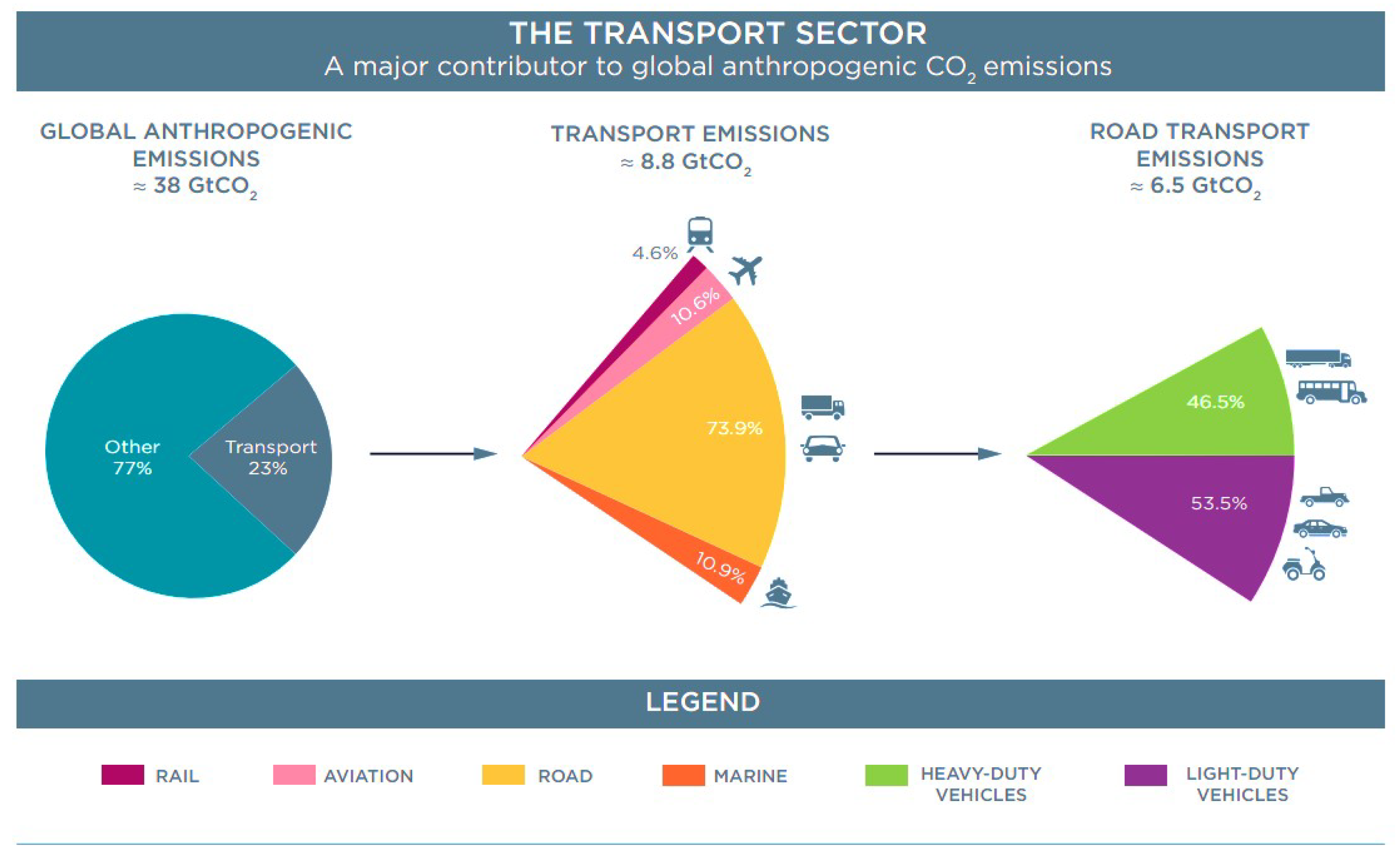
According to IPCC Guideline, there are two types of cargo trucks: light-duty vehicles (LDVs) and heavy-duty vehicles (HDVs) [11], as shown in Figure 1. As the global anthropogenic emission chart illustrates, the transportation accounts for 23% of global anthropogenic emissions, while the road transport emissions account for 73.9% of all transportation, LDVs and HDVs account for 46.5% of road transportation emissions.

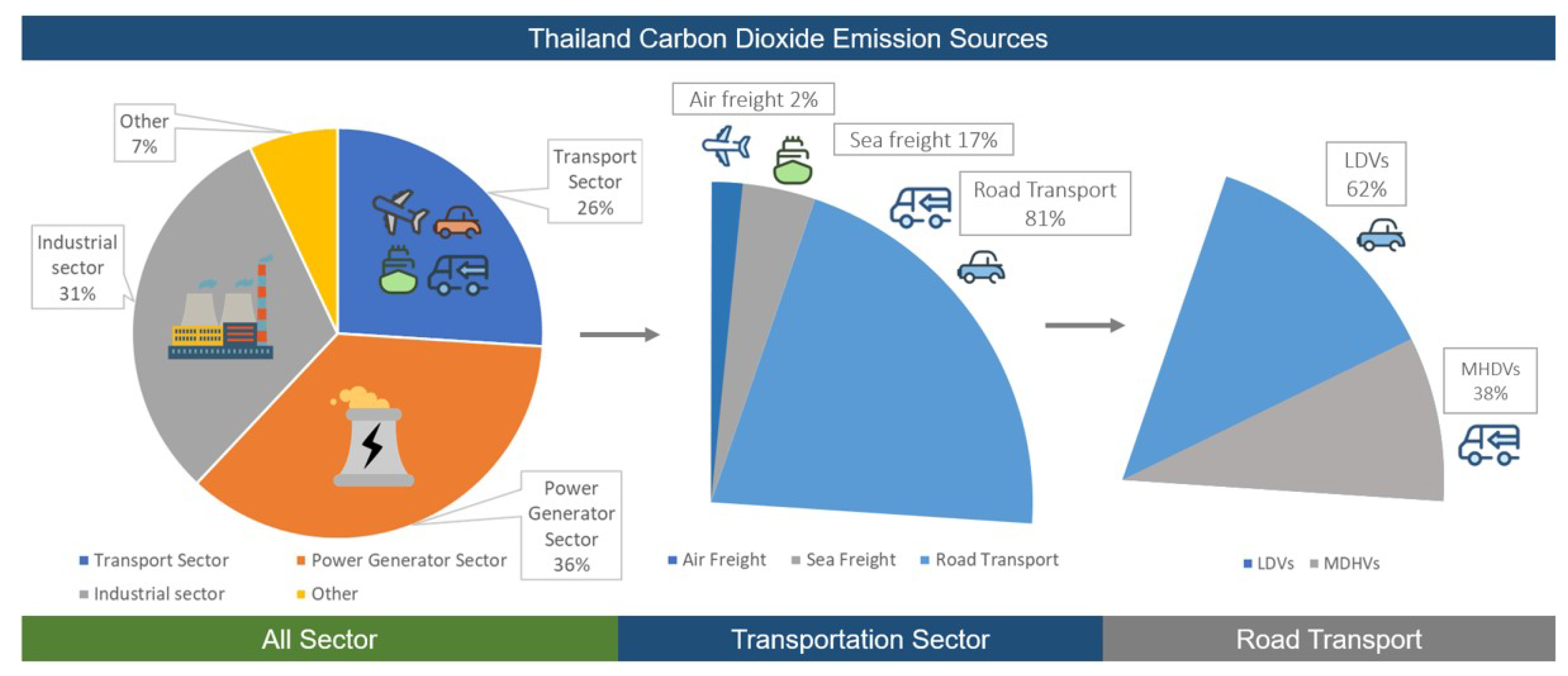
Regarding the sector of CO${}_2$ emission sources from the Thailand transportation chart (Figure 2), it is shown that HDVs account for 38.13% of all vehicles registered, higher than the usual range of 5–20% found in other countries. However, HDVs in Thailand account for 30–70% of CO${}_2$ emission in the country.

With the types of vehicles in

Table 1. Cargo vehicle types used for inland cargo transportation in Thailand.

Cargo Vehicle Types	Gross Vehicle Weight (GVW.)
Light-Duty Vehicles (LDVs)	GVW between 3500 kg–15,000 kg
Medium-Duty Vehicles (MDVs)	GVW between between 15,001 kg–30,000 kg
Heavy-Duty Vehicles (HDVs)	GVW 30,000 kg or more

concerned clarified, studying CO${}_2$ emission level of this type of vehicle using the chassis dynamometer method is impractical due to the substantial cost involved, forcing most studies to collect data through computer simulation instead. The programs include, for example, a simulation developed in the US named “Greenhouse Emission Model” (GEM,) and a vehicle-dynamic-based simulation named “Vehicles Energy Calculation Tool (VECTOR)” [12] developed in the EU. This paper’s focus is on the estimation of CO${}_2$ emission by these vehicles using actual collected data factoring in RSC levels. Thailand’s current estimation method for CO${}_2$ emission by land vehicles used by the Office of Transport and Traffic Policy and Planning (OTP) Ministry of Transport (MOT) only estimates the amount of vehicles in each using traffic density data and calculating that against average fuel consumption rates to find the estimate of CO${}_2$ emission in a given area. This method, however, may prove inaccurate, taking into account Thailand’s actual geographical variety. By estimating CO${}_2$ emission of an engine’s combustion without taking into account the road slope conditions, the resulting estimation of carbon dioxide emission will be lower than the approach where CO${}_2$ emission is calculated with the road slope condition considered.

This study aims to develop the CO${}_2$ emission coefficient for MHDVs in Thailand with varying topography, using actual collected and mapping data from the selected sample groups of vehicles. The data collected from global positioning system (GPS) and electronic control unit (ECU) will then be calculated factoring in geographic information system (GIS) information including slope, distance, traffic, weight and fuel consumption along the route. The coefficient of emission will then be calculated using multiple linear regression method. CO${}_2$ emission estimation for each area is then produced and used in analyzing the health impacts residents in each area are susceptible to. The studies also creates carbon maps with high risks of health effect and propose the policy and plans to manage the transport traffic in each area for alleviation for the populace affected by such emission.

2. Carbon Dioxide Emission (CO${}_{\mathbf{2}}$) and Road Slope Condition

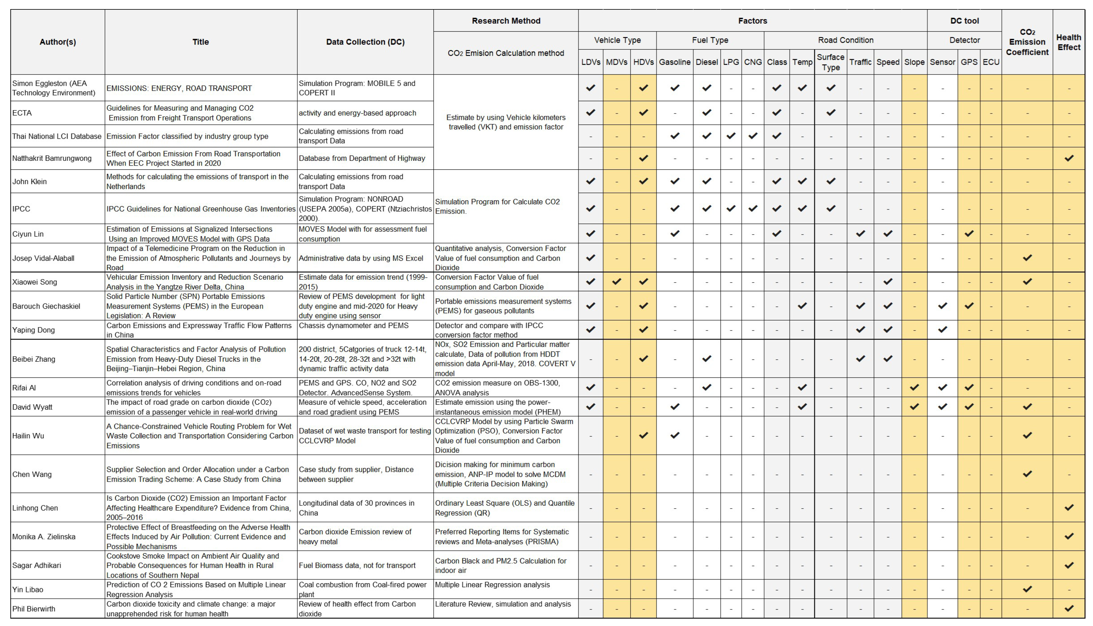
Since CO${}_2$ emission is a major cause of pollution, many research articles are proposed in these decades. Eggleston [13] on CO${}_2$ emission primarily uses MOBILE 5 and COPERT II simulation programs to estimate emission levels. These programs are capable of taking into account vehicle types including LDVs and HDVs using gasoline and diesel fuel types, different road types and different surface types. IPCC [14] produced the guidelines for national greenhouse gas inventories, which calculate CO${}_2$ emission using the simulation program NONROAD (USEPA 2005a), and COPERT (Ntziachristos 2000). In 2011, European Chemical Transport Association (ECTA) [15] developed the activity and energy-based data collection approach. Thai National Life Cycle Inventory Database [16] recognized that different cargo load levels on vehicles are susceptible to different levels of CO${}_2$ emission, separating cargo load levels into full load, 75% load, half load and empty. Klein [17] devised a pollution calculation approach for vehicle emission in the Netherlands factoring in the number of cargo vehicles active using simulation programs wherein different temperatures are accounted for, and factoring in additional effects by HDVs. Lin [18] study estimation of emissions at signalized intersections using an improved Motor Vehicle Emission Simulator (MOVES) Model with GPS Data is one to begin incorporating GPS data, which helped in producing a more accurate emission estimation than methods that only factor in numbers of vehicles which can better serve as a foundation for further environmental management planning.

This coincides with the trend in 2019 to focus more on the environmental side of the matter, with Vidal-Alaball [19] also proposing utilizing the telemedicine program to reduce the amount of air pollution created by road traffic, factoring in only emission by vehicles used by medical units and professionals to provide medical services. Song [20], as well, produced a record detailing emission by vehicles from 1999–2015 that can be used in estimating the future CO${}_2$ emission trend.

Giechaskiel [21] followed suit releasing a review of literature concerning the development of portable emissions measurement systems (PEMS) for the light-duty engine in Europe, with PEMS being developed to also support the heavy-duty engine in 2020. A study by Zhang [22] was then published in 2019 focusing on pollution from NO${}_x$, SO${}_2$ and particulate matter (PM) released by heavy-duty diesel trucks (HDDTs) in China, within which the economical and societal factors are factored in to estimate the actual pollution level caused by such transports. Then, in 2019, Bamrungwong [23,24,25] conducted a study on calculation of CO${}_2$ emission by road transportation and its estimated environmental impact when the eastern economic corridor (EEC) comes into effect in 2020. The study, however, factors in only the number of vehicles already active in the target area and predicts the actual number of vehicles when EEC begins using the growth rate of the government-supported new s-curve as a reference, with pollution statistics collected to be used in planning for measures to combat health effects residents of the EEC area are predicted to suffer from. Wu [26] developed the chance-constrained low-carbon vehicle routing problem (CCLCVRP) Model by using particle swarm optimization (PSO), using CO${}_2$ emission in selecting routes for wet waste collection and transportation with the goal being selecting the most appropriate routes and those that will least contribute to CO${}_2$ emission. Conversely, a study by Wang [27], Chen [28], Zielińska [29] and Adhikari [30], focuses more on CO${}_2$ emission and the subsequent pollution by industrial plants, with an emphasis on health effects potentially suffered by residents of the areas in the vicinity of these plants.

Libao [31] predicted CO${}_2$ from coal power plants using multiple linear regression analyses and compared the results of the fuel characteristics coefficient comparison with assessing CO${}_2$ emissions using the IPCC algorithm and method of coal consumption rate. Dong [32], conducted a study on fuel consumption and traffic volume information under various traffic flow patterns. The proposed carbon emission model has quantitative efficiency of carbon emission of vehicles under different traffic flow patterns. The goal is to provide information to support and become a valid reference for managing expressway operations and low-carbon expressway construction projects in the future. Al-rifai [33] studied the impact of road grade, vehicle speed and vehicle type on CO, NO${}_2$, SO${}_2$ and total volatile organic compound (TVOC) emission on the urban road in Jordan by studying at 0%, 2%, 4% and 6% sharpness using analysis of variance (ANOVA analysis). The grade parameter contributed the most to the rate of emissions compared to the other parameters of a gasoline vehicles. Wyatt [34] studied the impact of road grade on CO${}_2$ emission of a passenger vehicle in real-world driving, measure of vehicle speed, acceleration and road gradient. The exhaust CO${}_2$ emissions as measured by use of the OBS-1300 are captured on volumetric basis. The summary of the CO${}_2$ emission review is shown in Figure 3.

The air pollution in urban areas is mainly caused by transportation, and so it is necessary to assess pollutant exhaust emissions from vehicles especially mobile source. However, the current assessment of CO${}_2$ emission is incomplete because of the lack of consideration the road slope condition which is one of the significant factors. Evidently, no studies have yet to consider the different road slope levels of different areas for MHDVs as a factor that influences CO${}_2$ emission of vehicles and the subsequent air pollution this emission produces, which in turn continues on to be a primary cause of the global warming phenomenon through greenhouse gases accumulation, and a considerable health hazard to residents of affected areas in the form of potential lung cancer and increases the risk of bladder cancer [10].

This study aims to develop the CO${}_2$ emission coefficient for MHDVs in Thailand against varying topography, which consist of the road data, slope, distance, traffic, weight and fuel consumption along the transportation route. The coefficient of emission is then calculated using multiple linear regression analysis and validated by Huber–White standard errors for heteroscedasticity. The CO${}_2$ emission estimate for each route of the Asian highway is then produced and used in analyzing the health impacts residents in each area are susceptible to. The studies also propose carbon dioxide maps of areas with high risks of health effect and propose the policy and plans to manage the transport traffic in each area for alleviation for the populace effected by such emission.

3. Health Effect of CO${}_{\mathbf{2}}$ Emission

CO${}_2$, aside from being a major cause of the greenhouse effect which leads to global warming, also poses a serious airborne health hazard for those subjected to it. There are various studies on the health effects of CO${}_2$ focusing on emission by various sectors including agriculture, coal mining, food manufacturing, transportation and communication (among others, totaling at 26 industries). From said studies, the transportation sector is one to consume the most fuel, with the projected amount of CO${}_2$ emission by 2030 growing to 30% higher than the amount emitted in 2010. A study by the US National Library of Medicine suggests that affects of short term exposure to high levels of CO${}_2$ include suffocation by displacement of air, incapacitation and unconsciousness, headaches, vertigo and double visions, inability to concentrate, tinnitus and seizures, with a high amount of CO${}_2$ being breathed in posing a life-threatening danger. Documented health effects from breathing in CO${}_2$ at concentrations below 1% by P.N. Bierwirth [35] can be found in the Figure 4 below.

4. Methodology

4.1. Research Methodology

This study focuses on the CO${}_2$ coefficient value calculated from actual collected data, using information gathered by GPS tracking and ECU system of medium- and heavy-duty vehicles (MHDVs) moving through various geographically diverse areas with different elevations. The collected data include statistics on fuel consumption rate of these vehicles for each RSC level which is then calculated into CO${}_2$ coefficient showing CO${}_2$ emission for each RSC level.

The results are then compared to the calculations mostly used in previous studies, wherein the average value of CO${}_2$ emission per kilometer traveled is used. The resulting CO${}_2$ coefficient value is then used to analyze the health ramifications of residents in each area (Figure 5).

4.2. Data Collection and Processing

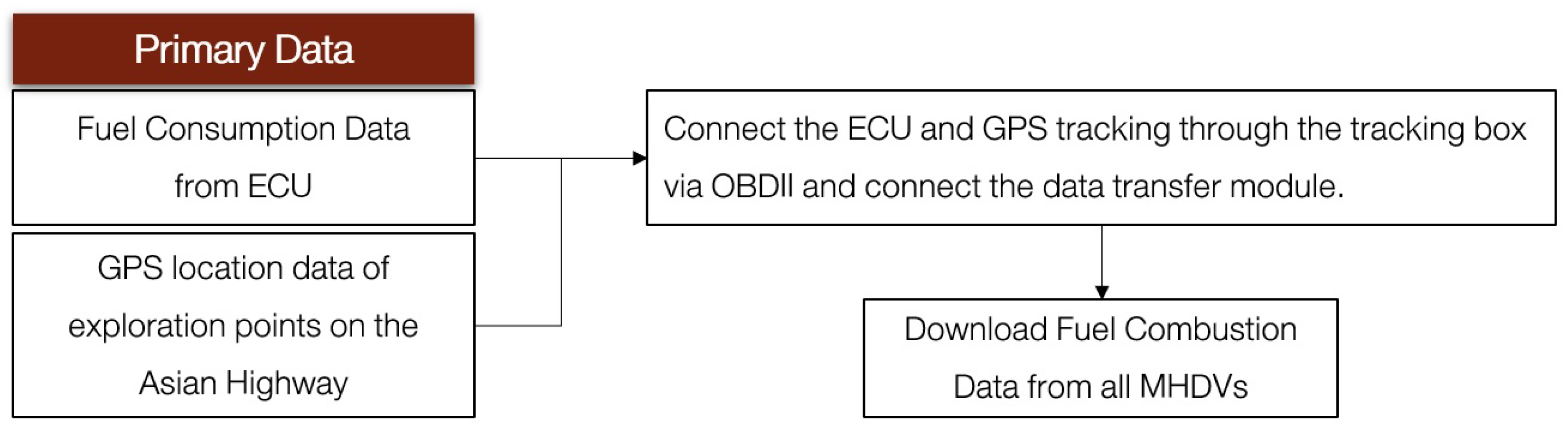
This section describes the process of collecting data for this research. The data are divided into 2 parts, which are primary data collection and secondary data collection.

Primary data collection consists of pre-fuel consumption data including Exploration Point, GPS position and distance in all road slope. The data are then analyzed against fuel consumption data of MHDVs (Figure 6) collected using GPS and cellular module.

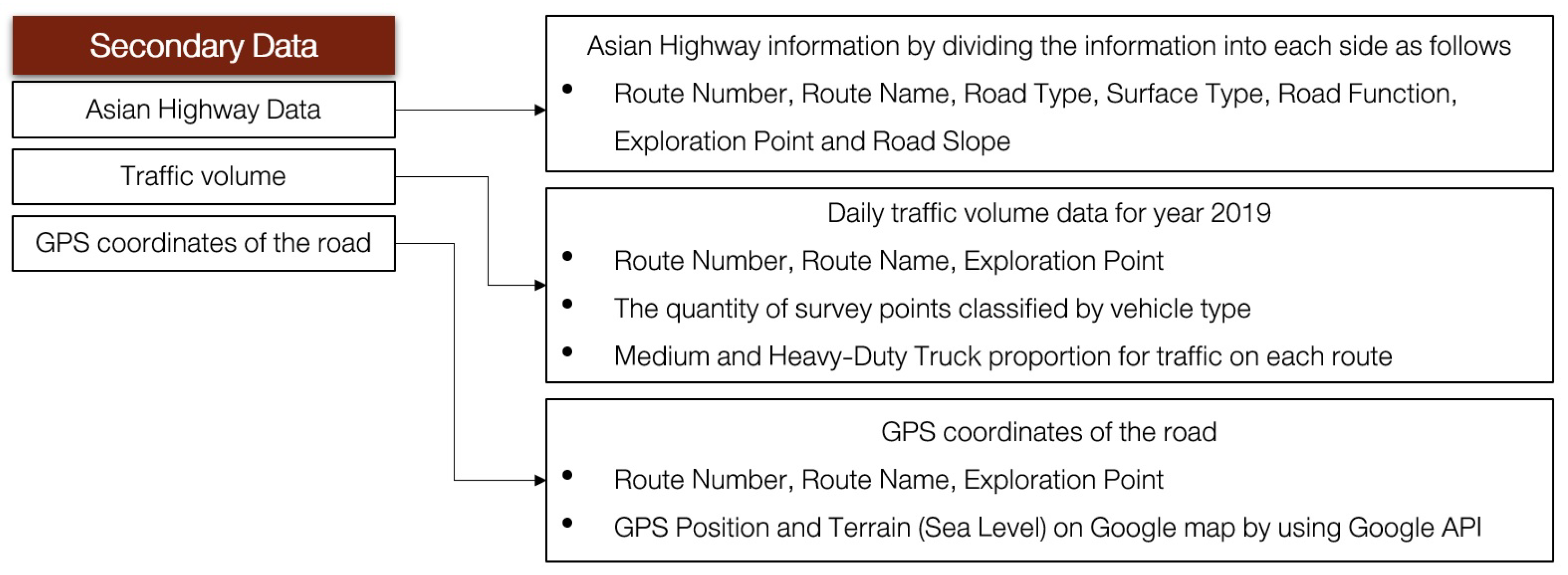
Secondary data collection includes data of traffic volumes on Asian highways used to calculate the amount of CO${}_2$ emitted on Asian highway. Vehicles are divided into 4 types including passenger car, LDVs, MDVs and HDVs (Figure 7).

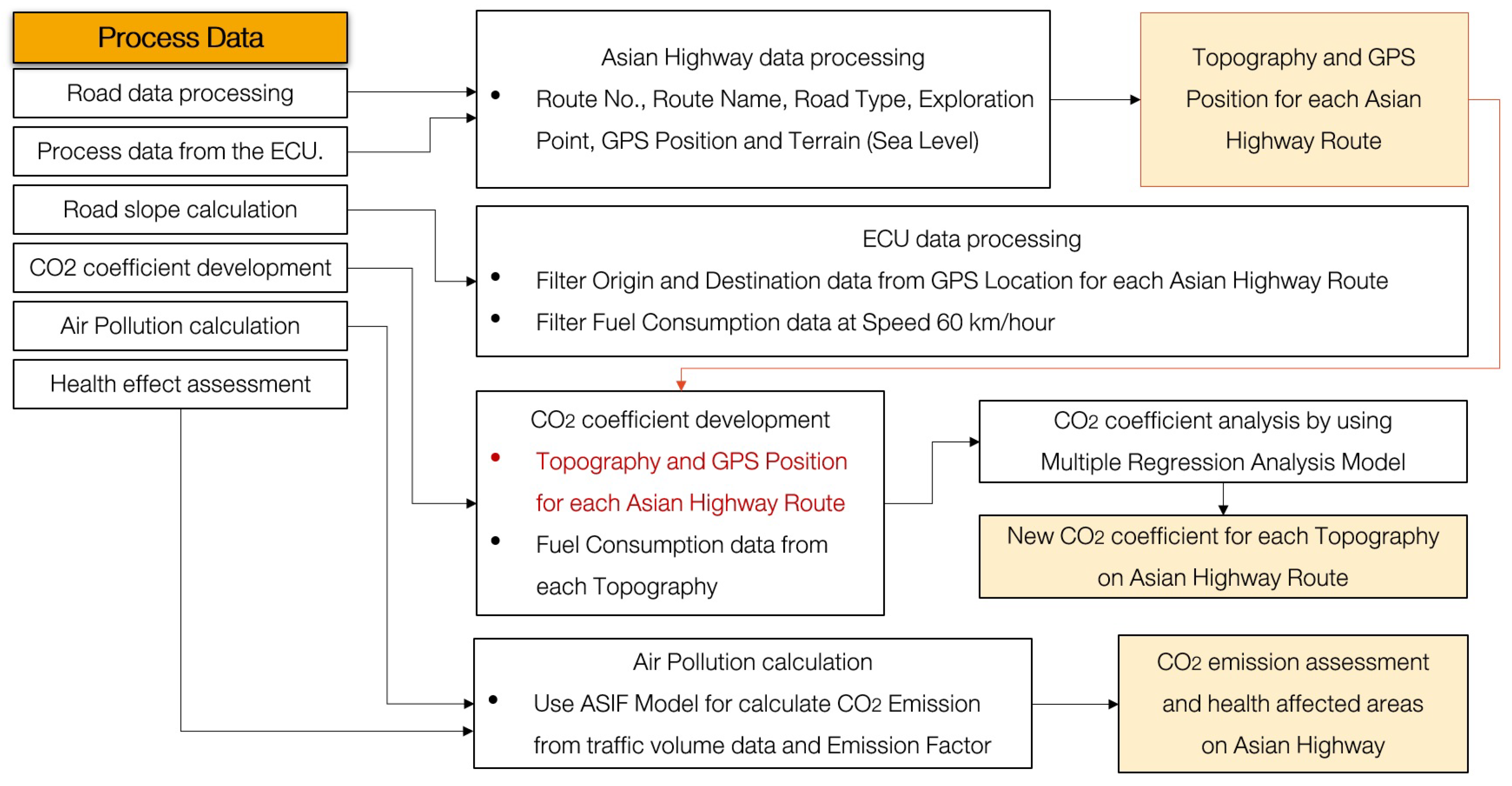
4.3. Data Processing

Once the primary and secondary data have been obtained, the two types of data are then used to develop CO${}_2$ coefficient values and calculate the amount of CO${}_2$ on the Asian highway. Afterwards, the amount of CO${}_2$ emission is used to calculate the CO${}_2$ concentration in the air for use in the analysis of the health impact to the area’s populace (Figure 8).

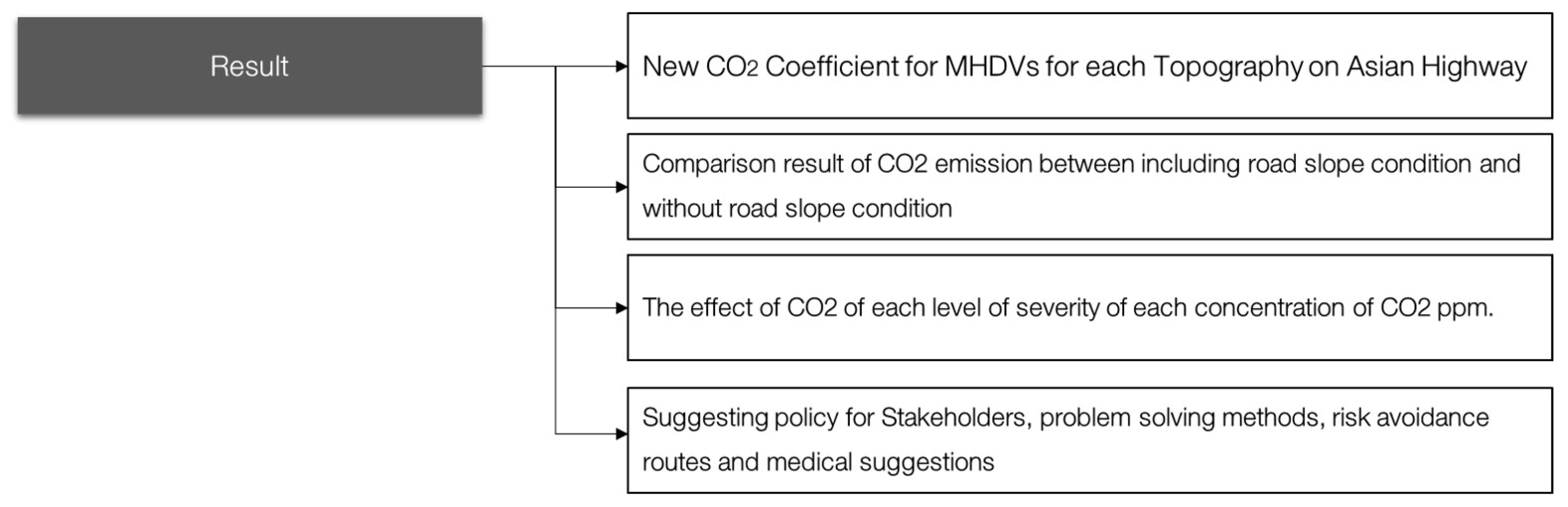
Then, two sets of data contrasting each other are produced, one being the calculation of CO${}_2$ emission considering slope condition, and the other being the same but with no consideration of road slopes, both using IPCC method for calculate CO${}_2$ emission from the traffic volume on the Asian highway and analyzing issues and ways of solving them by using the Asian highway avoidance route to study the avoidance route at high concentrations of CO${}_2$ ppm (Figure 9).

The resulting data are then used to form the basis of suggestions to stakeholders in order to create alternative risk-avoidant routes and medical solutions (Figure 10).

4.4. Multiple Linear Regression Validated Heteroscedasticity by Robust Standard Error

Actual CO${}_2$ emission data are collected from sample vehicles traversing through different terrains, which are then processed and compared using multiple linear regression analysis in order to produce the CO${}_2$ coefficient value. The resulting CO${}_2$ coefficient value is then tested for validity using robust standard error (Huber–White standard errors approach) for heteroscedasticity.

Multiple regression is a statistical technique using multiple descriptive variables to predict the of a variable’s response results. The purpose of multiple linear regression (MLR) is to model a linear relationship between explanatory variables and a response variable.

The formula for multiple linear regression is

$$y_i={\lambda }_0+{\lambda }_1{x}_{i1}+{\lambda }_2{x}_{i2}+\dots {\lambda }_p{x}_{ip}+\in$$

(1)

where, for i = 0,1,2,3,4,5,6:

$y_i$ = dependent variable,

$x_i$ = explanatory variables,

${\lambda }_0$ = y-intercept (constant term),

${\lambda }_p$ = slope coefficients for each explanatory variable,

∈ the model’s error term (also know as the residual).

Linear regression is a function that allows an analyst or statistician to make predictions about one variable based on the information that is known about another variable. Linear regression can be used in the case of two continuous variables, an independent variable and a dependent variable. The independent variable is the parameter that is used to calculate the dependent variable or outcome. A multiple regression model extends to several explanatory variables.

In econometric, a common test for heteroscedasticity is the White test, which begins by allowing the heteroscedasticity process to be a function of one or more of your independent variables. It is similar to the Breusch–Pagan test, but the White test allows the independent variable to have a nonlinear and interactive effect on the error variance.

Huber–White standard errors approach is a statistical test that establishes whether the variance of the errors in a regression model is constant: that is for heteroscedasticity. White proposed to add the squares and cross products of all independent variables in Equation (2):

The White test is based on the estimation of the following:

$${\widehat{\epsilon }}^2={\lambda }_0+{\lambda }_1{x}_{i1}+\dots {\lambda }_p{x}_{ip}+{\lambda }_{p+1}{x}_{ip}^2+\dots +{\lambda }_{2p}{x}_{ip}^2+{\lambda }_{2p+1}\left(x_{i_1}{x}_{i2}\right)+\dots +u_i$$

(2)

Alternately, a White test can be performed by estimating

$${\widehat{\epsilon }}^2={\delta }_0+{\delta }_1{\widehat{Y}}_i^2+{\delta }_2{\widehat{Y}}_i^2$$

(3)

where ${\widehat{Y}}_i$ represents the predicted value from

$${\widehat{y}}_i={\widehat{\lambda }}_0+{\widehat{\lambda }}_1{x}_{i1}+\dots +{\widehat{\lambda }}_p{x}_{ip}$$

(4)

Analysis of the multiple regression model with road slope condition calculations shows that the result is increasing variant, the error terms are heteroscedasticity and validated by Huber–White standard errors in order to get the most accurate coefficient.

4.5. CO${}_2$ Emission Equation

The current CO${}_2$ emission equation used to calculate the amount of pollution created by actual traffic and vehicles on the road, the following formula is used [11]:

$$Emission=\sum _{abcd}\left(\begin{array}{c}E{F}_{abcd}·Activit{y}_{abcd}\end{array}\right)$$

(5)

where:

Emission = Total CO${}_2$ emission from road transport (KgCO${}_2$),

EF = Emission factor, as mass per unit of activity rate,

Activity: activity rate (fuel consumed or distance traveled),

a = fuel type (diesel, gasoline, natural gas, liquefied petroleum gas),

b = vehicle type (passenger car, LDVs, MDVs, HDVs, etc.),

c = emission control,

d = road type (e.g., urban, rural, arterial, motorway, highway).

As with the current CO${}_2$ emission from Equation (5), the d variable only calculates CO${}_2$ emission based on the type of road as surface, etc. This research purposes that road slope condition of the route traversed by MHDVs contributes to the emission under the type of road variable (t), and must be considered if the accurate estimation of such emission is to be achieved. To calculate the CO${}_2$ coefficient value of each RSC level, each road is separated into various sections using the collected data, then each of these sections are given an estimate of RSC level. For the Asian highway, 5522 km of which is located within Thailand’s border, this study separates the road into 9 routes, with 55 checkpoints 100 km apart from each other. Once complete structural data of the Asian highway in Thailand are collected, the data are analyzed in order to find each route’s RSC levels.

Once the RSC level of each checkpoint is obtained, the data are calculated against the GPS data of the test vehicles for their fuel consumption rates. The result is the fuel consumption rate for each RSC level of the road. The resulting fuel consumption rates are then further analyzed in order to estimate the CO${}_2$ emission levels for each % slope, for all RSC levels. With CO${}_2$ emission levels for 1. Flat ground (0% slope) and 2. RSC level at 1–6 % slope, the results are compared using percentage difference method contrasting data for RSC areas with that for flat grounds. Once the RSC levels for all routes are identified, then next step is to calculate the CO${}_2$ emission level for each checkpoint of the road in relation to the RSC level of said checkpoint, and contrasting the result with the statistics of cargo trucks in use on the road in 2019 provided by the Department of Highways. The result from the assessment of CO${}_2$ emission on Asian highway in each range of total routes shows the volume of carbon dioxide emission and it will be consequently applied to further health effect analysis.

4.6. Materials

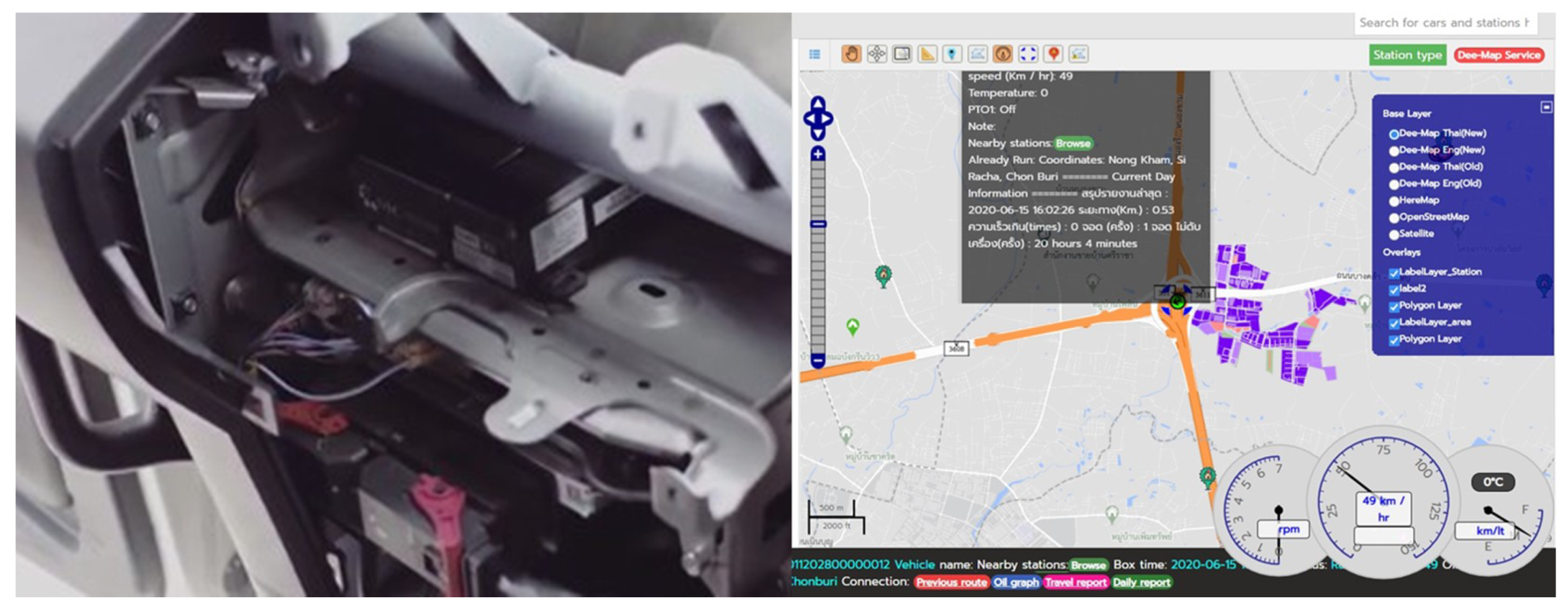
Equipment used in this study includes an ECU, used to collect data through OBD2 port from each vehicles of the sample group of 57 cargo trucks (MHDVs). Of these, 25 are MDVs, and 32 are HDVs. Each vehicle was equipped with an ECU, and its fuel consumption rate data are linked with its GPS data, as shown in Figure 11.

Then, the data are processed as follows

• Data retrieved from a vehicle are compared against location history in the database.
• Calculation is made to determine the fuel consumption rate for each area, using RSC level data of each area of the Asian highway and its corresponding RSC level for reference, and Exploration Points provided by the Department of Highways to determine the exact GPS value of the area. (In fact, the resulting travel data will specify the exact GPS positions of the points of origin and destination).
• A table showing the fuel consumption rate for each RSC level is then created to further calculate the CO${}_2$ coefficient value.

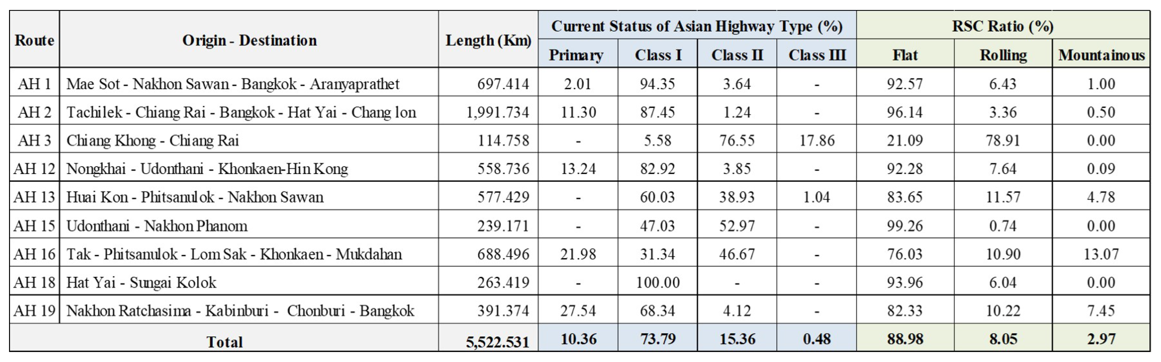
4.7. Current Status and RSC of Asian Highway

The assessment method of CO${}_2$ emission on Asian highway began in the study of Thailand’s Asian highway network [46], where the Highway is divided into 9 routes. These are AH1, AH2, AH3, AH12, AH13, AH15, AH16, AH18 and AH19. The total length of these sections is 5522 km (Figure 12).

From Figure 12, the study shows that a majority of the Asian highway consists of class I road (73.79%), class II road (15.36%) and primary road (10.36%). Class II road is a minority, meaning that most of the highway area targeted by this study is under the surface of concrete and asphalt, with similar or identical surface hardness (Standard No. DH-S 416/2013) [47].

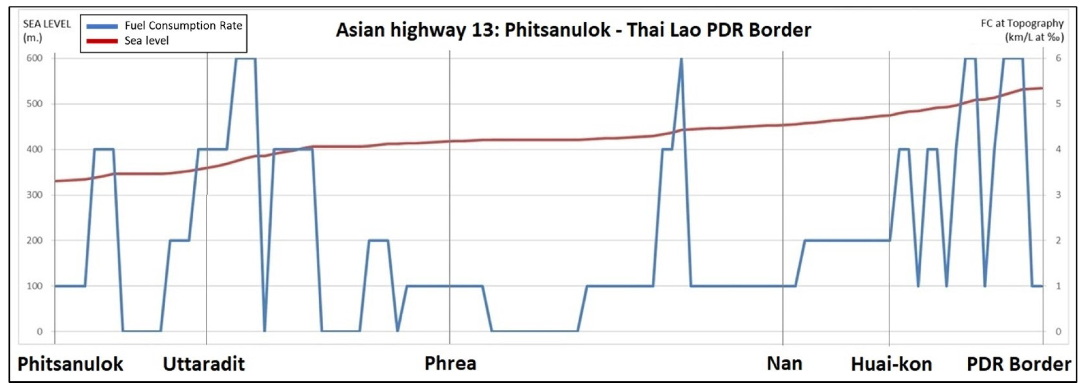
From the study, it can be gathered that, for CO${}_2$ emission throughout route AH13 starting from Pitsanulok province and ending at Chiang Khong Border checkpoint, the slope level continues to increase. This, in turn, referencing the chart displaying correlation between sea level and fuel combustion rate from ECU for route AH13, indicates that higher incline levels exponentially increase fuel consumption rate of a vehicle. Based on fuel combustion rate and CO${}_2$ emission data, the CO${}_2$ emission level of each incline level can be determined.

Figure 13 shows an example of data retrieved from ECUs linked to GPS, which are more inclusive than the data in Figure 9, including the collection of the Truck Footprint, which is a vehicle’s travel history detailing its specific position in each area, as well as its real-time fuel consumption rate. These data are to be used to calculate the CO${}_2$ coefficient value for each RSC level as shown in Figure 14.

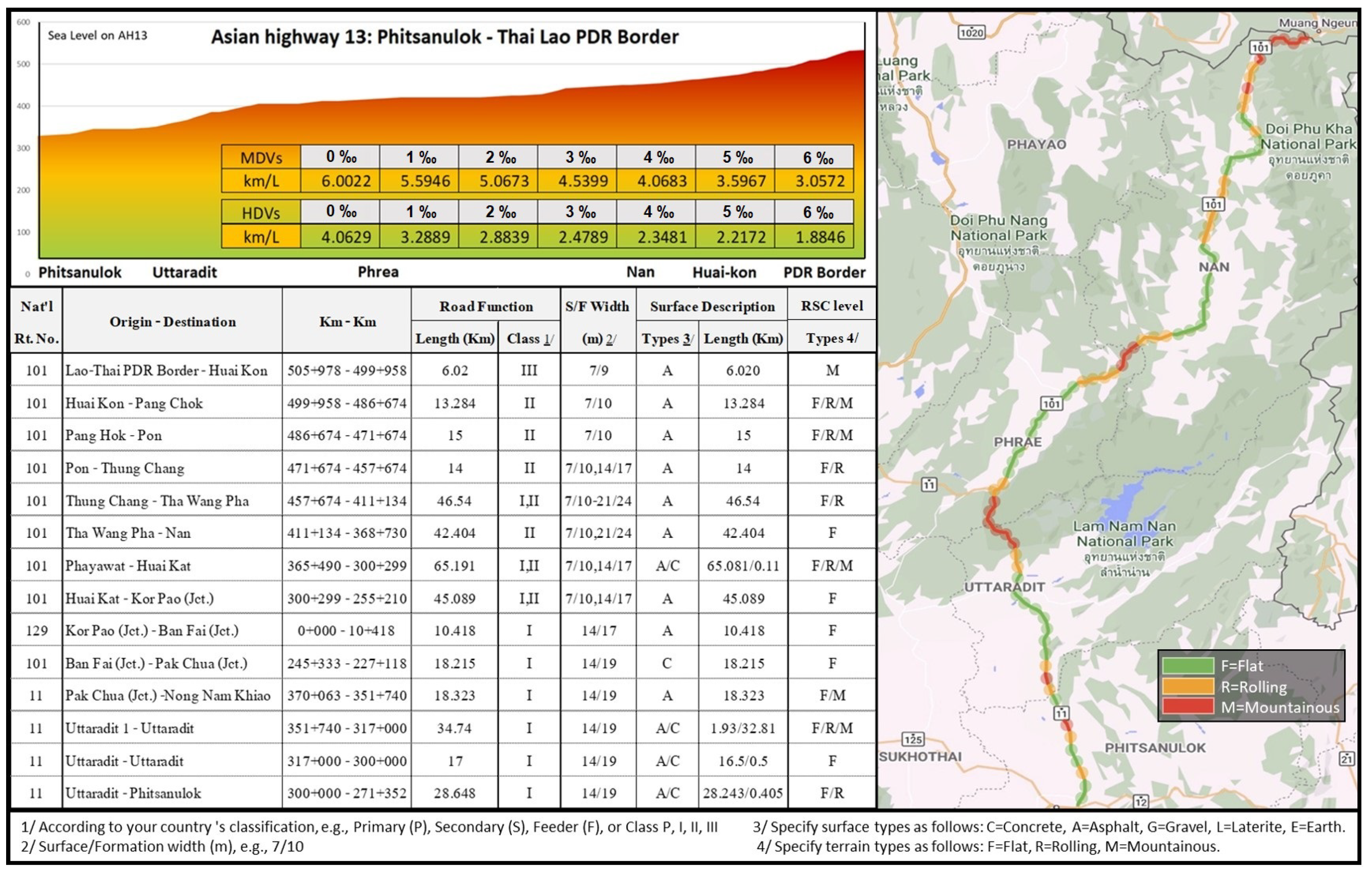
RSC levels can be separated into 3 categories including Flat, Rolling and Mountainous, with RSC levels from 0–6‰. CO${}_2$ emission with RSC collected data includes dates, types of vehicles based on their licenses, distance covered for different areas and average fuel consumption rates for all routes. These data are archived as travel history and are to be used for further route-specific analyses.

4.8. CO${}_2$ Emission Assessment

Calculation of carbon dioxide throughout the journey can be calculated using the following equation

$$TotalC{O}_{2}Emission=(FC·EF·D·V)$$

(6)

FC = fuel consumption per km. (L./Km.)

EF = CO${}_2$ emission coefficient (KgCO${}_2$/Liter of fuel) depends on type of fuel.

D = distance (km.)

V = number of vehicles.

From collecting and mapping the data from the Department of Highways, GPS and ECU consisting of the road data, slope and distance resulting in CO${}_2$ emissions in units KgCO${}_2$/Km.

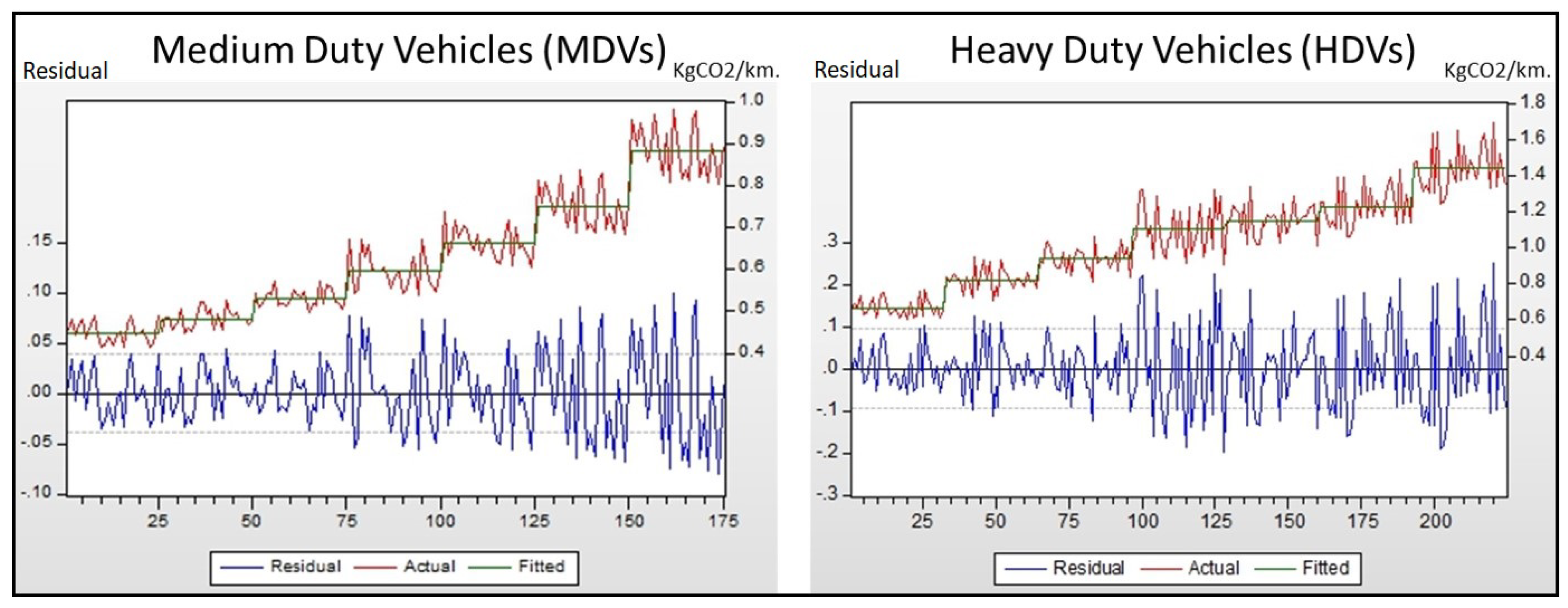
Once the MHDV’s CO${}_2$ emission data has been collected for each slope road, the data obtained are then plotted in the graph to analyze the data format in order to find the most suitable model for calculation as shown in Figure 15.

Based on data from the MDVs and HDVs’ database analyzed with multiple regression methods, the coefficient values can be defined by the estimate regression equation as follows:

$$Y_{MDVs}=0.449+0.032x_1+0.082x_2+0.146x_3+0.214x_4+0.302x_5+0.434x_6$$

(7)

$$Y_{HDVs}=0.665+0.157x_1+0.271x_2+0.435x_3+0.486x_4+0.556x_5+0.772x_6$$

(8)

where the $X_i$ are explanatory variables for value of CO${}_2$ emission for each road slope ($Y_i$):

• at 0 % slope, explanatory variables of $x_1$,$x_2$,$x_3$,$x_4$,$x_5$,$x_6$ = 0,
• at 1 % slope, explanatory variables of $x_1$ = 1, otherwise = 0,
• at 2 % slope, explanatory variables of $x_2$ = 1, otherwise = 0,
• at 3 % slope, explanatory variables of $x_3$ = 1, otherwise = 0,
• at 4 % slope, explanatory variables of $x_4$ = 1, otherwise = 0,
• at 5 % slope, explanatory variables of $x_5$ = 1, otherwise = 0,
• at 6 % slope, explanatory variables of $x_6$ = 1, otherwise = 0.

From Equations (7) and (8), $y_i$ = CO${}_2$ emission per 1 km. at i % slope, then

CO${}_2$ emission of MHDV per 1 km. at i% slope (unit: KgCO${}_2$/km.)

• at 0 % slope, $y_{0\left(MDV\right)}$ = 0.449,          $y_{0\left(HDV\right)}$ = 0.665
• at 1 % slope, $y_{1\left(MDV\right)}$ = 0.449 + 0.032 = 0.481,  $y_{1\left(HDV\right)}$ = 0.665 + 0.157 = 0.822
• at 2 % slope, $y_{2\left(MDV\right)}$ = 0.449 + 0.082 = 0.531,  $y_{2\left(HDV\right)}$ = 0.665 + 0.271 = 0.936
• at 3 % slope, $y_{3\left(MDV\right)}$ = 0.449 + 0.146 = 0.595,  $y_{3\left(HDV\right)}$ = 0.665 + 0.435 = 1.100
• at 4 % slope, $y_{4\left(MDV\right)}$ = 0.449 + 0.214 = 0.663,  $y_{4\left(HDV\right)}$ = 0.665 + 0.486 = 1.151
• at 5 % slope, $y_{5\left(MDV\right)}$ = 0.449 + 0.302 = 0.751,  $y_{5\left(HDV\right)}$ = 0.665 + 0.556 = 1.221
• at 6 % slope, $y_{6\left(MDV\right)}$ = 0.449 + 0.434 = 0.883,  $y_{6\left(HDV\right)}$ = 0.665 + 0.772 = 1.437

Then, the CO${}_2$ emission all route from Equation (6) can be written in a generic form as equation

$${\widehat{y}}_i=\sum _{i=0}^6{y}_i{D}_i=\sum _{i=0}^{6}EF·F{C}_i·D_i$$

(9)

where EF is the CO${}_2$ emission coefficient dependent on type of fuel, and $D_i$ is the total distances (km) at i % slope, i = 1, 2, 3, 4, 5, 6.

All $y_i$ are composed of $y_0$ while $EF·F{C}_0$, when the $F{C}_0$ of fuel consumption at 0% slope = 1.669 for MDV and 0.247 for HDV (liter/km.)

Therefore, the total CO${}_2$ emission with RSC of MHDVs is equal to

$${\widehat{y}}_{i\left(MDV\right)}=EF·F{C}_0\left(D_0+1.0713·D_1+1.1826·D_2+1.3252·D_3+1.4766·D_4+1.6726·D_5+1.9666·D_6\right)$$

(10)

$${\widehat{y}}_{i\left(HDV\right)}=EF·F{C}_0\left(D_0+1.2361·D_1+1.4075·D_2+1.6541·D_3+1.7308·D_4+1.8361·D_5+2.1609·D_6\right)$$

(11)

Formulate in the generic form

$${\widehat{y}}_i=EF·F{C}_0\left({\lambda }_0·D_0+{\lambda }_1·D_1+{\lambda }_2·D_2+\dots +{\lambda }_6·D_6\right)$$

(12)

or

$${\widehat{y}}_i=\sum _{i=0}^6({\lambda }_i·F{C}_0·EF·D_i)\left(KgC{O}_2\right)$$

(13)

However, the total CO${}_2$ emission includes traffic of MHDVs, therefore

$${\widehat{y}}_i=\sum _{i=0}^6({\lambda }_i·F{C}_0·EF·D_i·V_i)\left(KgC{O}_2\right)$$

(14)

where

${\widehat{y}}_i$ is total CO${}_2$ emission (KgCO${}_2$),

${\lambda }_i$ is CO${}_2$ emission coefficient,

$F{C}_0$ is fuel consumption (liter/km.),

EF is emission coefficient of fuel (KgCO${}_2$),

$D_i$ is the total distance (km.) at i % Slope, i = 0,1,2,3,4,5,6.

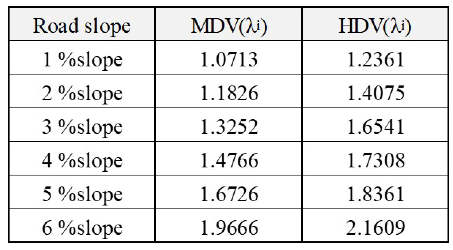
Thus, the summary of the MHDV coefficients are shown in Figure 16.

From Figure 16 it is shown that the CO${}_2$ emission values of MDV for 1–6% slope are greater than flat road (0% slope) at 1.0713, 1.1826, 1.3252, 1.4766, 1.6726 and 1.9666 times, respectively. For HDV, the CO${}_2$ emission values for 1–6% slope are greater than flat road (0% slope) at 1.2361, 1.4075, 1.6541, 1.7308, 1.8361 and 2.1609 times, respectively.

4.9. Studying Health Effects

The study of health effects of CO${}_2$ emission is a continuation of the empirical study on carbon emission from engine combustion of cargo transport vehicles, and the study of articles relating to CO${}_2$ emission coefficients, with the aim to provide data to health professionals. In-depth interviews are used as the favored approach, employing a naturalistic inquiry method. Participants of this process are provided a pollution estimate of each checkpoint and CO${}_2$ density in the air (given in the from of CO${}_2$ part per million: ppm)

CO${}_2$ concentrate calculation is as follows;

CO${}_2$ in 1 ppm = 1.80 mg CO${}_2$/$m_3$

So,

$$C{O}_{2}ppm=\left(\frac{mgC{O}_2}{1.8·D·L·2.5·96}\right)$$

(15)

where

mgCO${}_2$ = Molecular weight of CO${}_2$ (mg).

1.8 = 1.8 mg. CO${}_2$/$m^3$ = 1 ppm of CO${}_2$.

D = Distances: Range of road exploration in meter unit (m).

L = Length: Length of road exploration in meter unit (m).

2.5 = The height used to calculate CO${}_2$ density (m).

96 = CO${}_2$ per a quarter of an hour (min).

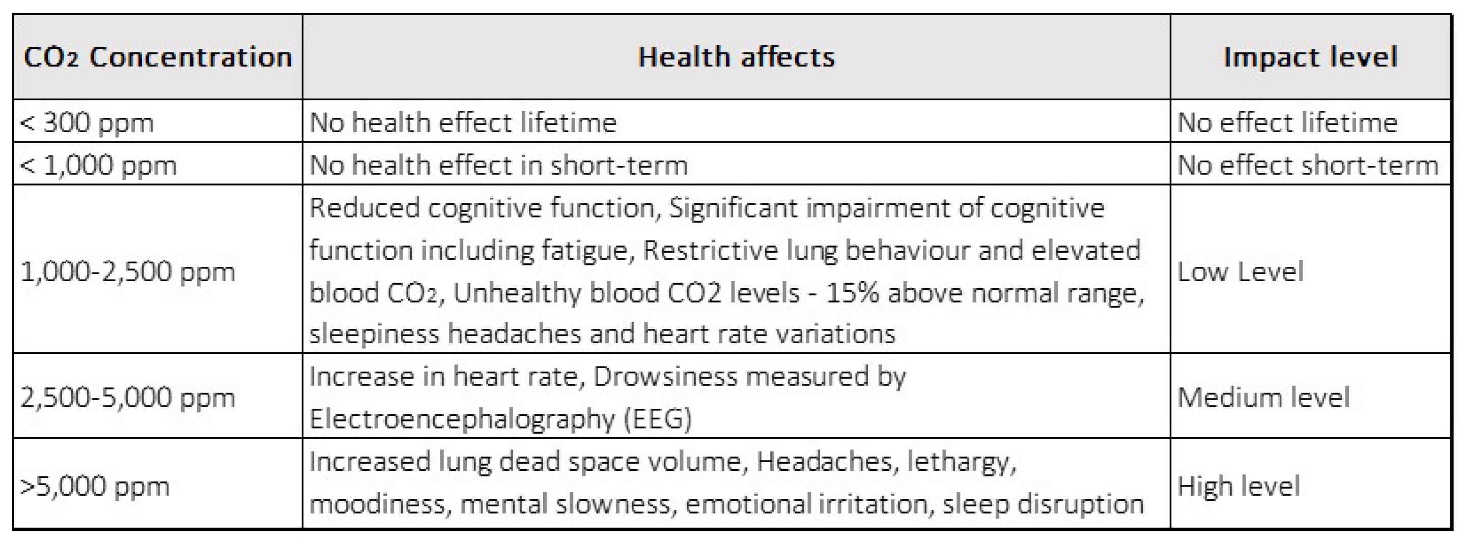
When calculating the amount of CO${}_2$ concentration in the air, the data obtained are analyzed with the results in Figure 17 for use in the analysis of the affects of CO${}_2$ emission.

4.10. CO${}_2$ Emission Assessment for Asian Highway

The different CO${}_2$ coefficient values for different RSC levels of terrains point to an average of high CO${}_2$ emission in the immediate areas of the Asian highway, enough to potentially cause health complications to the residents of said areas. This study hence focuses on the number of MHDVs to determine the CO${}_2$ emission levels on the Asian highway and the health effects to the residents, as shown in Figure 18.

It can be observed from the above diagram that emission estimations in certain areas are done so without taking into account the slopes. These estimations are therefore inaccurate and may prove to be of no use, or even harmful, to the populace in the areas when it comes to health concern management.

4.11. Health Effect Result

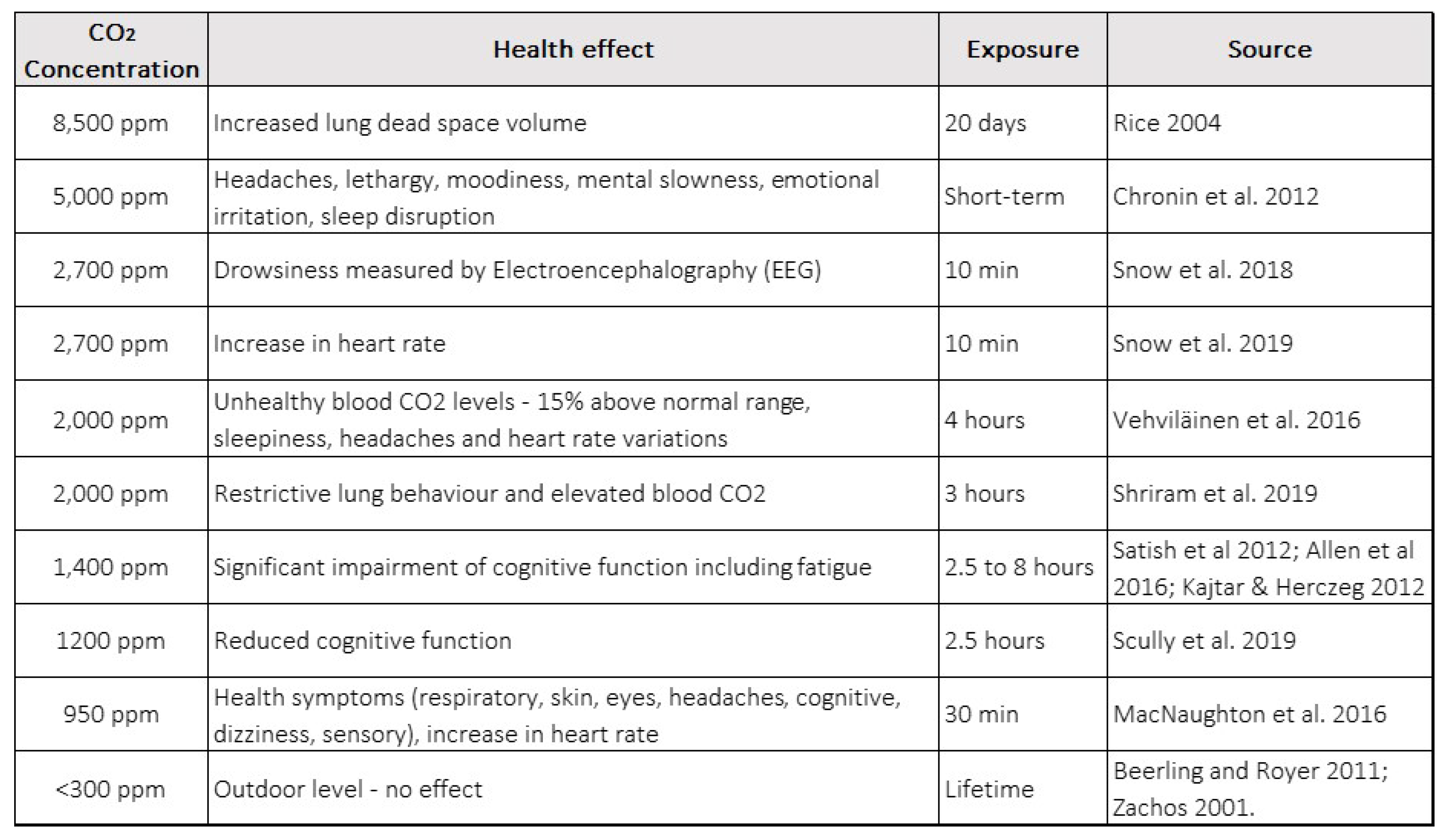
Studies of health effect from CO${}_2$ emission on the Asian highway by physicians shows that when residents along the road transport area inhale a certain amount of carbon dioxide, carbon dioxide binds to hemoglobin 20 times more in erythrocyte than oxygen. This will lessen the ability of blood to carry oxygen from the lungs to other tissues of the body or reduce oxygen in the blood. If we inhale 2500–5000 ppm of carbon dioxide continuously for 15 min, it may decrease our ability to see, induce headache or cause drowsiness and tiredness; if we are to inhale constantly for 8–12 h, this may progress to abnormal movement [48], severe headaches and slight intoxication depending on the exposure time; and if we are exposed repeatedly for 6 weeks, it will affect heart and brain structures. However, if a person inhales 40,000 ppm consistently for only 5 min, he or she may be in a risk of death. Even though oxygen is necessary to carry out cell functions, it is not the lack of oxygen that stimulates breathing. Breathing is stimulated by an excess of CO${}_2$. If an individual breathes too slowly (bradypnea), does not breathe deeply enough (dyspnea) or is exposed to excessive CO${}_2$ levels, too much CO${}_2$ can build up. This causes increased breathing and the other physiological responses discussed above [49].

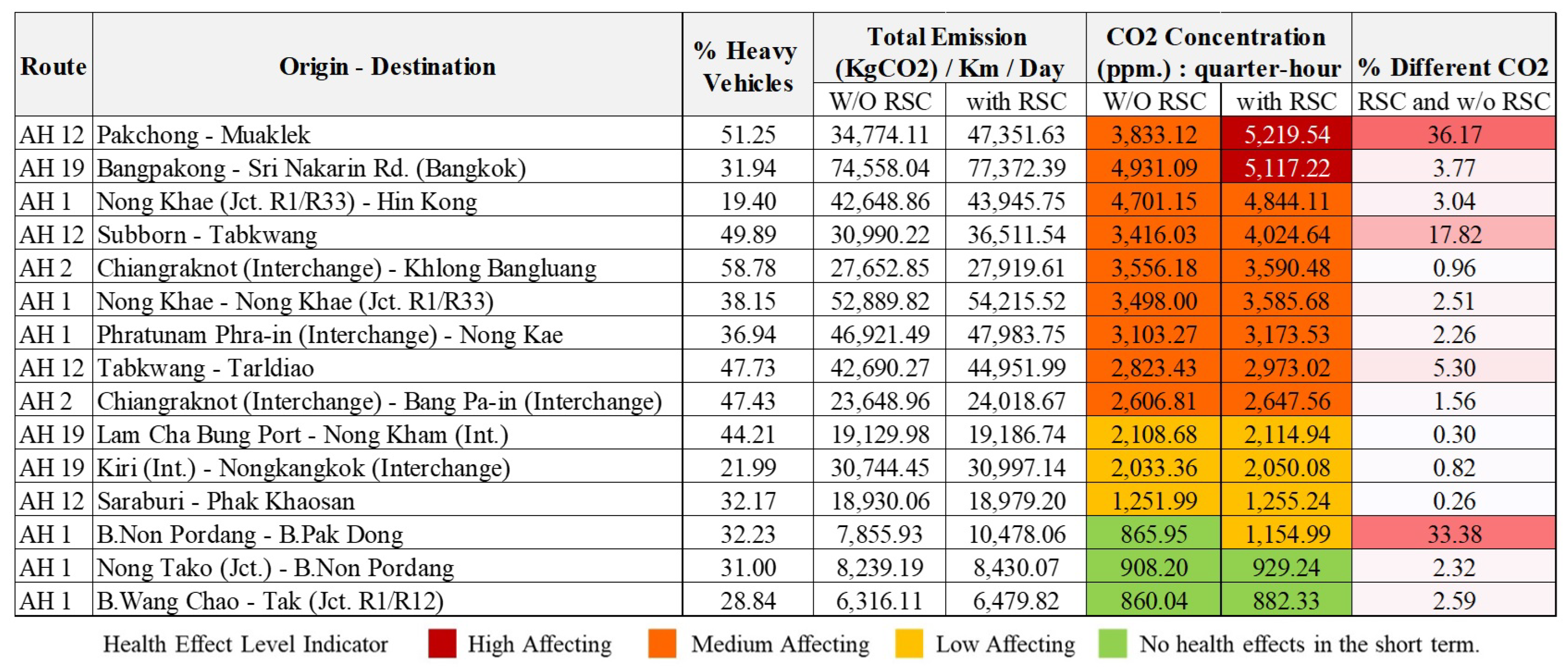
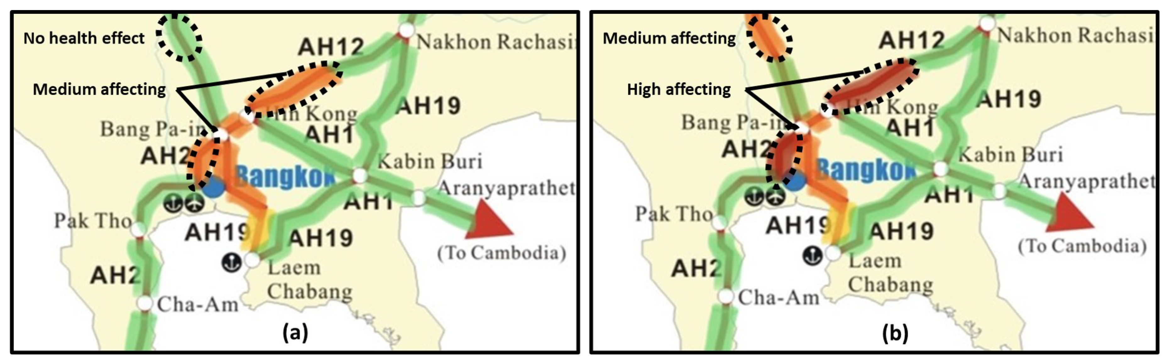
The map (Figure 19) shows that residents of areas with low RSC levels or none are subject to low or no health effects. Conversely, areas with high RSC levels and areas with high traffic amount are subject to CO${}_2$ emission of high concentration. For example, AH12 route, which begins at Muaklek district, Saraburi province, and ends at Pakchong district, Nakhon Ratchasima province, consists mainly of a long climb uphill, and a large number of vehicles, making up of 36.17% of those that use the route, are MHDVs, making it one of the areas in Thailand with the residents most likely to be affected health-wise by CO${}_2$ emission. This is especially true during festivals, where traffic buildups are an issue even more prevalent.

5. Conclusions and Suggestions

The development of a CO${}_2$ emission coefficient with varying topography conditions for MHDVs addition to consideration of health effects on the people was conducted. The study area is the part of the Asian highway in Thailand passing through different, highly geographically diverse regions of the country in order to analyze and create the model showing the CO${}_2$ emission coefficient in each road slope. The coefficient of CO${}_2$ emission will be determined by the multiple linear regression and validated by Huber–White robust standard errors for heteroscedasticity. Results from the study of CO${}_2$ emission by calculating a road slope condition resulting in a higher CO${}_2$ emission than 36.17% without a road slope condition, which affects the ability to formulate policies and plans for populations affected by pollution that is less than reasonable have been.

Stakeholders must be accountable for reducing CO${}_2$ emission on all parts of the Asian highway and the health ramifications implicit with the issue. The public sector can approach alleviating this issue by way of adjusting cargo truck routes and operating time to prevent cargo trucks, particularly MHDVs, from operating during peak hours with high level of traffic. Aid programs should also be offered by both the public sector and private entities accountable for the emission. Suggestions and opinions by experts and the writer are collected herein and offered as follows.

Suggestions for the government: The government should have in place a policy on protection and developing a plan against the pollution created by land cargo transports as depicted in this study. It should also offer aid to those residing in areas affected by high emission of CO${}_2$ by the aforementioned transports, and offer legal support for those suffering long term effects of air pollution. Moreover, a tax should be imposed on cargo trucks entering areas with high CO${}_2$ amount to encourage drivers to take alternative, less CO${}_2$-dense routes, which in this instance will have lower tax rates imposed upon (Carbon Tax for Road Transport). In this vein, alternative routes to reduce traffic density and help with avoiding precipitous areas should also be built. Tax for agencies working to lessen the emission of CO${}_2$ by transports likewise should also be reduced.

Suggestions for the private sector: The private sector should take responsibility in reducing carbon emission by transport vehicles and to manage transport routes to the effect that traffic-congested routes and precipitous areas are less clogged. A back-hauling system should also be in place to lessen the amount of carbon emission.

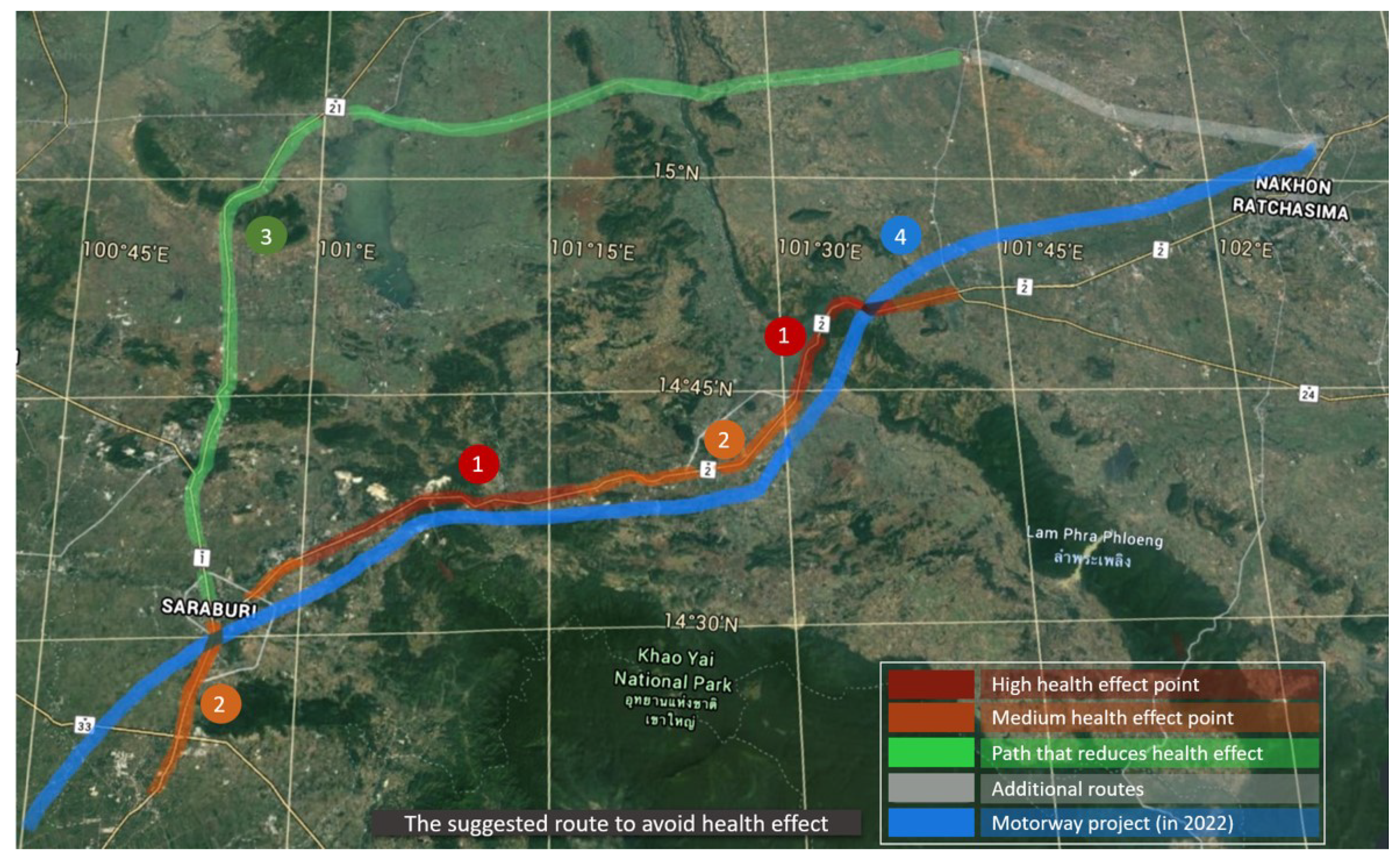
As shown in the health impact minimization map for cargo transport routes (Figure 20), the red (Circle no.1) and orange (Circle no.2) lines indicate spots where residents near the Asian highway are subjected to health risks from CO${}_2$ emission. The green line (Circle no.3) represents the route that leads into Road number 21 (Saraburi–Lomsak), which then leads into Road number 2256 heading towards Nakhon Ratchasima. The route is slated in the future to merge back into the Asian highway eventually but as of now a direct route into the province is unavailable. This study suggests that a road be constructed along the white line covering 44 km distance as an alternative route. The blue line (Circle no.4) represents the planned motorway by the Department of Highways estimated to begin operating from 2022–2023. The motorway, however, will present tolls for usage, which will add to cargo transportation expenses. 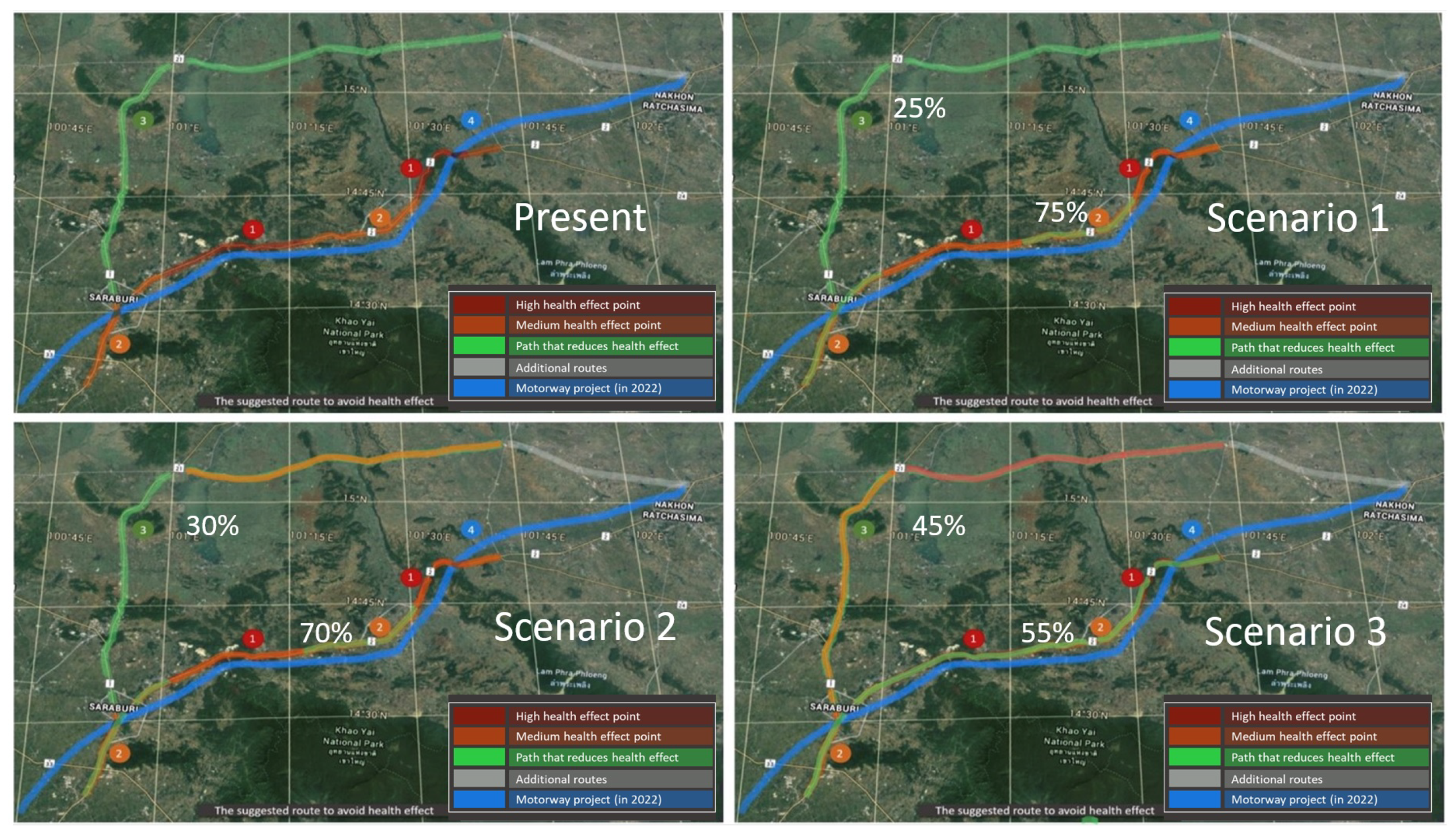Using the alternative route, which will ideally not be subjected to toll, should help alleviating this issue and reducing CO${}_2$ emission by MHDVs (Figure 21), with health risk level projected to reduce from high to medium level should 25% of vehicles (Scenario 1) travel on alternative routes instead, and to low level should 30% of vehicles (Scenario 2) do so. Should more than 45% of vehicles (Scenario 3) choose to traverse the alternative route, however, residents along the route may begin to be subjected to increased health risks instead.

The study thus suggests that specific time windows for usage of the Asian highway be imposed, and that more than one alternative suggested route be created for traveling during festivals or heavy traffic conditions to reduce the health affect from CO${}_2$ on the main highway. Vehicle emission should also be rigorously checked before vehicles are allowed into the area, and entrepreneurs should be made conscious of health impacts cargo transportations bring to the populace of the areas their cargos travel through.