A Trade-off Analysis of Economic and Environmental Aspects of a Disruption Based Closed-Loop Supply Chain Network

Abstract

Closed-loop supply chain networks are gaining research popularity due to environmental, economic and social concerns. Such networks are primarily designed to overcome carbon footprints and to retrieve end of life products from customers. This study considers a multi echelon closed-loop supply chain in the presence of machine disruption. A multi-objective model is presented to optimize the total cost, the total time and emissions in a closed-loop supply chain network. The aim is to analyze the trade-off between the objectives of cost, time, and emissions and how these decisions are impacted by the selection of different available machines. A number of solution approaches are tested on a case study from the tire industry. The results suggest the improved performance of the hybrid heuristic and the importance of controlling disruption in a closed-loop supply chain network. Furthermore, there is a trade-off between the different objective functions which can help the decision maker to choose a particular solution according to the preference of an organization. Finally, conclusion and future research avenues are provided.

1. Introduction

Supply chain management (SCM) integrates different parties involved in the business network. It considers various aspects of decisions such as acquisition of raw materials and the delivery of finished goods [1]. Traditionally, supply chains involved the analysis primarily based on cost; however, recent advents have demonstrated the integration of several other aspects such as environmental sustainability and well-being of employees, to name a few [2]. Besides, a constant pressure is being exerted by government agencies and society to limit the environmental footprints of production and supply chain networks [3]. The supply chain is thought to be the leading source of global warming, environment degradation and carbon emissions [4].

Traditionally, the forward supply chain was focused to provide the goods to end consumers using cost-effective and responsive mechanisms. Such supply chains were based on forward logistics without taking into account the end-of-life (EOL) treatment of products retrieved from the end consumer. As logistics has received more attention from law makers and customers, businesses have embedded the reverse logistics into their practices. The reverse logistics can take a cross-company dimension as well where in-house operations such as return, disassembly and remanufacturing are prioritized. This is done to reduce environmental impact and improve the carbon footprint of businesses.

Van Hoek et al. [5] argue that the inclusion of reverse logistics is not enough, and businesses need to incorporate the idea of green supply chains to become more sustainable in their practices. The leap from reverse logistics to the supply chain concept is defined by a shift from reactive approaches to value seeking approaches. For instance, the manufacturing system can react to the environmental footprint concerns by taking initiatives for mitigating the emissions, etc. On the other hand, if the environmental aspects are considered as an opportunity to seek value, the businesses can take a pro-active approach to define its long-term vision for green supply chains. Thus, a sustainable edge, cost cutting and innovation base can be formed.

The green supply chain starts at the supply source and its scope extends towards the packaging, product transportation, distribution and end customer. Furthermore, at the end of life, the products are called back to the manufacturing system where they are re-manufactured or used for value extraction. Thus, a holistic perspective of supply chain system is taken into account which provides a long lasting impact on green practices. Such perspective ensures that the manufacturing system takes full responsibility for product re-use to play a strategic role in minimizing the environmental impacts by integrating environmental activities.

Together, the forward and reverse logistics make up a closed-loop supply chain (CLSC). An effective CLSC needs to be managed, controlled and run to enhance the profit values and reduce the anticipated costs throughout the life cycle of the product [6]. The manufacturing system can consider various challenges which hinder the boost of an efficient CLSC. These challenges can be in the form of facility deployment, designing the product flow, cost reduction and environmental protection [7,8]. Though the CLSC analysis has been considered from different viewpoints, the analysis of time, number of machines, production disruption and different market niche, to name a few, are missing in the concerned literature.

This study designs a sustainable CLSC network by integrating various aspects related to sustainability and environmental factors. The aim of this study is two-fold. First, a keyword analysis is presented to highlight existing gapes in the relevant literature. Secondly, a deterministic model and solution approaches are proposed to fill the existing gapes. We analyze a CLSC problem by considering different echelons/level in the form of supplier, production, cross-dock, distribution, customer location, repository for return, secondary and tertiary markets. An important aspect of the analysis is to consider the production disruption which can potentially generate in-house waste and thus a liability on the part of manufacturer. A multi-objective model is presented for optimizing the total cost, the total time and the carbon emission. We want to understand the trade-off between the three objectives and how they are impacted when a different set of disruptive machines are selected.

The rest of the study is organized as follows. Section 2 offers a detailed literature related to different aspects of the considered problem. Section 3 provides the problem statement and mathematical model. Section 4 contains the detail of different solution approaches. Section 5 provides the results and discussions. Section 6 contains the conclusion and future research recommendations.

2. Literature Review

2.1. Closed-Loop Supply Chain

A CLSC can be defined as “a supply chain system entailing design and implementation for enhancing the useful value throughout the product life cycle while dynamically extracting value from different returned products” [3]. CLSC has been attaining research attention and recent comprehensive reviews to this field have been offered by [7,8,9]. There are different contributions offered towards the analysis of the CLSC network. For example, Pazhani et al. [10] proposed a multi-objective model that included the objectives of cost and efficiency to analyze the performance of a CLSC. The synthesis was based on decisions of locating warehouses, production and distribution of goods.

The environmental aspects have been receiving an increasing amount of research focus to cater the emission and footprint issues. There have been different contributions to analyze the environmental aspects of a CLSC. A multi-echelon CLSC was considered in [11] by using an incentive plan and retrieval of used products based on different quality levels. A multi-objective model was presented to optimize the total cost and the environmental impact of the CLSC. Yavari and Gerali [12] studied the CLSC for perishable goods by presenting and analyzing a multi-product, multi-period and multi-echelon model. A multi-objective model was presented to minimize the total cost and the environmental pollutants.

Soleimani et al. [13] analyzed the objectives of profit maximization, reduction of lost working days and environmental aspects. Different recycling strategies i.e., product, component and material recycling were analyzed using a genetic algorithm. Zhen et al. [14] proposed a stochastic bi-objective model to optimize the operating cost and environmental aspects of a CLSC network. A multi-echelon and low-carbon based network was designed that included the decisions regarding production, recovery, distribution, disassembly and customer locations. Zhalechian et al. [15] studied a sustainable CLSC problem and considered the aspects of CO₂ emission, fuel consumption and social concerns of a new job opening. Mohammed et al. [16] analyzed the environmental impact and total cost by proposing a multi-period and multi-product based CLSC. A trade-off was proposed between CO₂ emission and the cost of a supply chain network. Although an adequate amount of research has been offered towards the establishment of an efficient CLSC, there still is a dearth of literature to address the environmental concerns of CLSC, emission, etc. [17]. A detailed procedure was adopted to extensively analyze the concerned literature and it is discussed below.

Although supply chains are a classical subject, the debate on closed loop supply chains and their optimization efforts have been gaining attention in the past two decades. Thus, we collected the associated literature published in the last 20 years. We identified the list of articles, conferences, books and thesis in the databases of ProQuest and Scopus. The articles were sorted using the keyword of “closed loop supply chain” and further filtered using “optimization keyword”. The list of articles was shared with two experts to obtain an informed view on inclusion/exclusion of articles based on relevance to the current topic.

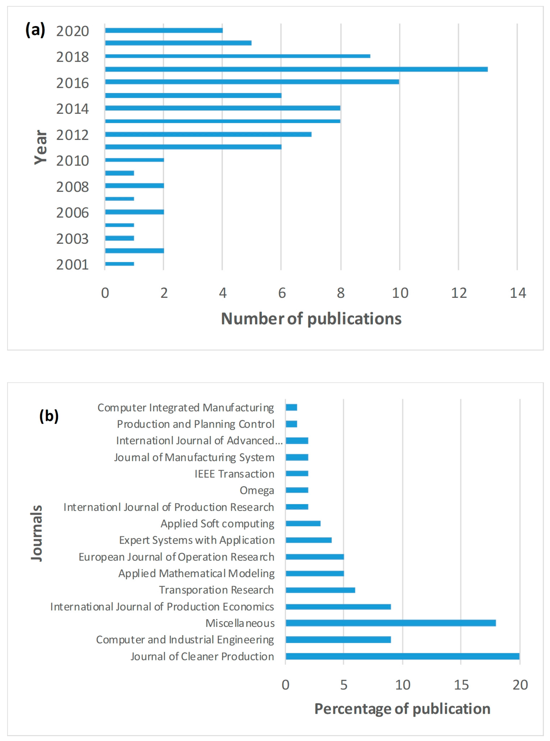
The distribution of accumulated literature with respect to the year of publication and journals is provided in Figure 1. From Figure 1a, we can observe that there has been a growing trend of publication, especially in the last 10 years. We expect that this trend will continue and extend in the next years. Figure 1b describes the percentage of publication in different journals. In particular, the Journal of Cleaner Production has the highest percentage of publication on optimization efforts in CLSC networks (20%), followed by Computer and Industrial Engineering (9%) and International Journal of Production Economics (9%).

Following this, each article was thoroughly analyzed using five (05) criteria. These criteria were: embedded factors, choice of objective function, solution approaches, additional aspects and the level of markets for products.

• The embedded factors include re-manufacturing, energy extraction and disposal.
• The selected choices of objective functions contain cost, environmental/social aspects and time.
• The selected articles were scrutinized against the solution approaches of heuristics, multi-heuristics and hybrid heuristics approaches.
• The additional set of aspects comprised the analysis of vehicle speed and disruption.
• The target markets were identified at three levels i.e., primary, secondary and tertiary market.
• The analysis results are presented in Figure 2. These are further discussed in the following sections.

2.2. Embedded Factors and Market Levels

The CLSC operates in a way to collect the products once they have completed their useful life. If the product is of adequate quality, it is re-manufactured to make it as good as (or almost as good as) a new product. Secondly, if the product is non-repairable, maximum level of energy is extracted from it which is subsequently fed to the production processes. Thirdly, the product is disposed of after acquiring energy from it, or if it is in such a poor state of quality that it cannot offer any useful amount of energy. Thus, the embedded factors considered here relates to re-manufacturing, energy extraction and disposal. The distribution of embedded factors is provided in Figure 2a. It can be observed that re-manufacturing is the most opted strategy adopted for returned products (56% articles) (refer to [18,19,20] etc.,) compared to energy extraction (8%) [21,22] and disposal (36%) [23,24]. It might be due to the fact that legislators and customers are constantly pushing for minimizing the carbon footprint of products through re-manufacturing. Similarly, there is a dearth of literature focusing on the integration of all three factors (e.g., [25,26,27,28]. This study considers the integration of the aforementioned factors in the CLSC analysis.

The market levels refer to the number of times the product is re-launched in different quality conditions. Initially, a perfect quality product is supplied to primary market and upon completion of the useful life, it is retrieved, refurbished and then supplied to the secondary market. The product launched in the secondary market is somewhat inferior in quality compared to the products launched in the primary market. We introduce the notion of tertiary market based on quality differentiation where the maximum amount of energy is attained and the remaining is disposed. The CLSC literature distribution according to market levels is provided in Figure 2d. As is obvious, most of the optimization studies in CLSC launch the products initially to the primary market (85%) [29,30] as opposed to distribution to secondary (14%) [31,32] and tertiary market (1%) [18]. The current study considers the three embedded factors and the three market levels for optimization analysis of the CLSC network.

2.3. Choice of Objective Functions and Additional Aspects

From the managerial perspective, it is important to support the design of a CLSC network by optimizing it against certain criteria. These criteria can be in the form of cost, time, responsiveness, etc. For the current analysis, we surveyed the associated literature with respect to the objectives of cost, environment and social aspects and time. The relevant results are provided in Figure 2b. Cost has been more often chosen as the choice of objective function to optimize the performance of a CLSC network (77%) [32,33,34]. The aspects of cost used in the analysis comprises, but are not limited to transportation, purchasing, re-manufacturing, capacity cost, etc. [23,35]. Until now, the concerned literature has lacked in analyzing the cost related to disruptive performance of machine. The proposed objective function of cost considers novel cost components related to failed and re-work products due to machine disruption.

Beside cost, the second choice of objective function is environment and social aspects (23%). The environmental aspects considered in the published literature are: energy spent, emissions, environmental impacts, trading price of carbon emission, etc. [25,36,37]. The social aspects considered for the CLSC optimization are based on the selection of a responsible supplier, societal development, job security and wages. etc. [27,28].

An important point to note is that none of the CLSC studies have optimized the network design on the basis of time. Time is an essential aspect of a production system/supply chain as it impacts the throughput and responsiveness towards the customers. This study performs a thorough analysis of time of CLSC by integrating components of transportation time between various echelons, production time, lost production time and re-work time.

We also reviewed the associated literature with respect to the additional aspects of vehicle speed and disruption. The aspect of vehicle speed plays a sensitive role in the performance of CLSC as beside other factors, it affects the time to deliver a product. The existing literature analyzes the vehicle speed; however, the sensitivity analysis of such parameters on the performance of the CLSC network performance is observed less often. Similarly, disruption in the supply chain can affect the performance of the latter and it has been analyzed in only a few studies. The existing literature considers disruptions such as supplier disruption and demand disruptions. Certain disruption related issues are also addressed in the open supply chain literature in the form of demand disruptions and manufacturing cost disruptions. To the best of our knowledge, none of the existing studies in the CLSC literature have addressed the issue of machine disruption. We posit that the machine may be disrupted due to inadequate maintenance and thus cannot meet the required level of optimal quality products. Thus, the number of machines is to be increased in order to cope with the required quantity.

2.4. Solution Approaches

A list of solution approaches can be found in the relevant literature for the optimization of CLSC problems. These approaches are in the form of exact solution approaches such as MIP/MILP based on solver/CPLEX and non-exact approaches such as genetic algorithms, Tabu search, simulated annealing, fuzzy approaches and memetic algorithm to name a few. The MIP and MILP are considered powerful approaches towards the analysis of CLSC performances [28]. The application of such methods can be found in [38,39,40,41].

The non-exact approaches can be highlighted as heuristics, multi-heuristics and hybrid solution approaches. In terms of heuristics/algorithms, genetic algorithm is the frequently used approach. For instance, Kannan et al. (2010) [42] used a genetic algorithm to formulate a strategy for retrieving the EOL products, distribution and inventory related tasks. The literature distribution of CLSC problems according to the adopted solution approaches is provided in Figure 2c. The application of heuristics (85%) have outnumbered the multi-heuristic approaches (7%) and hybrid solution approaches (8%). The application of heuristics to CLSC problems can be found in [43]. The multi-heuristics represent the application of multiple heuristics and their application can be found in [44]. The hybrid heuristic approaches combine two meta-heuristics into a unified approach and their application can be found in [45]. Given the fact that there is scarcity of application of multi-heuristics and hybrid approaches in the context of CLSC problems, this study uses two meta-heuristics and a hybrid solution approaches to solve the problem.

Based on the presented literature, the list of contributions offered by this study can be summarized as:

• A multi-objective analysis is presented to analyze the multiple levels of a closed-loop supply chain. The considered objectives are: the total cost, the total time and the carbon emissions.
• A consolidated analysis is presented by integrating the factors of re-manufacturing, energy extraction and disposal. Also, three market levels are considered for minimizing the level of waste.
• We examine the impact of machine disruption on the performance of CLSC. Also, the impact of vehicle speed on the transportation performance of a CLSC problem is presented.
• The solution is attained using multi-heuristics and hybrid approaches. Furthermore, three performance evaluation metrics are used to evaluate the solution efficiency of the considered approaches.
• The objective is to analyze the trade-off behavior of cost, time and emissions. In other words, how these decisions can be controlled while fulfilling customer demand. Secondly, in the presence of machine disruption, which production facility can help accomplishing an overall optimal solution.

3. Problem Statement

The considered problem involves the analysis of multiple levels of a closed-loop supply chain (CLSC) such as suppliers, production machines, cross-docking points, distribution points, customer locations, repository for return products, secondary and tertiary markets.

The schematic of problem is given in Figure 3 which describes the different levels in the CLSC. The flows i.e., forward, return, secondary and tertiary flows are denoted by different lines. We consider single supplier, single repository for return, single secondary market and a single tertiary market.

The supplier provides the raw materials to production machines for processing them into finished products. A distinct number of machines are available to process the products. Each machine j works perfectly well and is able to produce the quantity of production using its available capacity ca_j. However, due to inadequate maintenance, it starts disruption defined by probability value ${\lambda }_j$. Due to disruption, the state of the machine can be divided into “in-control” and “out-of-control” states. The production in the control state results in optimal quality products while the out-of-control state produces moderate quality products and failed products due to machine disruption. The failed units are discarded while the moderate quality products are re-worked to make them conforming. Since the production capacity is fixed, we select the minimum number of appropriate machines j to meet the demand quantity after discarding the failed units.

After production, the products are sent to cross-docking point for sorting and later dispatched to customer locations (m) through distribution points (l). At the end of life, the products are retrieved to the repository for return products (n). Here, the products are inspected and further divided into conforming and non-conforming units. The conforming units are of considerable quality and are re-manufactured at j and shipped to secondary market (o). The non-conforming products are in a bad quality state and these cannot be re-manufactured. Thus, they are shipped to the tertiary market where maximum energy is extracted out of them and the remaining are disposed as waste. The model details and objective functions are provided below.

Indices
i	set of suppliers	i = {1,2,…, I}
j	set of production machines	j = {1,2,…, J}
k	set of cross-docking points	k = {1,2,…, K}
l	set of distribution points	l = {1,2,…, L}
m	set of customer locations	m = {1,2,…, M}
n	set of repository for product return	n = {1,2,…, N}
o	set of secondary markets	o = {1,2,…, O}
p	set of tertiary markets	p = {1,2,…, P}
Parameters
$q_j$	quantity of raw materials fed to production machine j
$c_j$	cost of manufacturing per unit product on machine j
$c{e}_j$	cost of exploiting machine j
$t{p}_j$	per unit production time at j
$e_j$	per unit production energy used at j
$d{x}_{jk}$	distance between machine facility j and cross-dock point k
$c{e}_m$	carbon emitted during production per unit product
$c_{tv}$	carbon emitted during transportation per kilometer
$t{r}_c$	transportation cost per kilometer distance travelled
$Fc{a}_j$	feasible production capacity of machine j
$Nc{a}_j$	non-feasible production capacity of machine j
${\lambda }_j$	probability of machine disruption
$d{y}_{kl}$	distance between cross-dock point k and disruption point l
$r{w}_j$	cost of re-work at machine facility j
$c{w}_j$	failed product cost per unit due to machine disruption
$c{p}_p$	penalty cost of discarded product at tertiary market
$d{z}_{lm}$	distance between distribution point l and customer location m
$d{d}_{mn}$	distance between customer location m and respiratory n
$d{f}_{nj}$	distance between respiratory n and production facility j
$\Psi$	fraction of conforming products at n
$1-\Psi$	fraction of non-conforming products at n
$f$	fraction of non-conforming products used for energy extraction
$1-f$	fraction of non-conforming products discarded as waste
$d$	required level of demand
$V$	vehicle speed in kilometer per hour
$c{r}_m$	cost of re-manufacturing per unit
$ee$	energy extracted per unit product at tertiary market
$t{t}_j$	re-work time per unit product at production facility j
$tr{m}_j$	remanufacturing time per unit product at production facility j
$ew$	energy wasted due to carbon emission at tertiary market
$Z$	A big number
Decision variables
$M_j$	1, if machine facility j is used for production, else 0
$X_{jk}$	1, if products are shipped between j and k, else 0
$Y_{kl}$	1, if products are transported between k and l, else 0
$Z_{lm}$	1, if products are transported between l and m, else 0
$L_{mn}$	1, if m is used to transport products to n, else 0
$S_{jo}$	1, if products are launched into secondary market o, else 0
$N_{np}$	1, if products are sent to tertiary market, else 0
$NM$	number of machines required for production
$F_{nj}$	1, if conforming products are sent from n to j, else 0
$MN{M}_j$	Auxiliary variable
$XN{M}_j$	Auxiliary variable

3.1. Minimize Total Cost (TC)

The first objective is to minimize the total cost of the CLSC network. It comprises production cost, transportation cost, failed units cost and re-work cost, as given in (1). The expression for each cost component is discussed in detail.

$$TC=PC+TRC+FC+RC$$

(1)

3.1.1. Production Cost (PC)

PC expression calculates the cost of machine exploitation, production and re-manufacturing cost of return products. Its expression is given in (2) as:

$$PC={\displaystyle \sum _{j=1}^J{M}_j}.NM.c{e}_j+{\displaystyle \sum _{j=1}^J{M}_j}.c_j.q_j+{\displaystyle \sum _{j=1}^J{\displaystyle \sum _{n=1}^N{F}_{nj}}}.c_{rm}.\Psi .d$$

(2)

The first portion of PC expression calculates the machine exploitation cost of using a number of machines. For a perfectly working production system, the number of machines can be calculated as the ratio of demand to production capacity. On the other hand, we are considering the disruption in the machine which causes failed product units. Thus, the number of machines is calculated by subtracting the failed product units from the available capacity of machines. This ensures the availability of enough machines to produce the required level of optimal quality products. The relationship for number of machines (NM) is provided in (3) as:

$$NM={\displaystyle \sum _{j=1}^J{M}_j}.\left(\frac{d}{Fc{a}_j+(1-{\lambda }_j)Nc{a}_j}\right)$$

(3)

The second and third portions of the PC relationship respectively calculates the production and remanufacturing costs.

3.1.2. Transportation Cost (TRC)

The TRC expression calculates the cost of transportation between machine facilities, cross-docking, distribution points, customer locations and repository for return. The expression for TRC is given in (4) as:

$$\begin{array}{l}TRC={\displaystyle \sum _{k=1}^K{\displaystyle \sum _{j=1}^J{X}_{jk}.d{x}_{jk}.t{r}_c+}}{\displaystyle \sum _{l=1}^L{\displaystyle \sum _{k=1}^K{Y}_{kl}.d{y}_{kl}.t{r}_c+}}{\displaystyle \sum _{m=1}^M{\displaystyle \sum _{l=1}^L{Z}_{lm}.d{z}_{lm}.t{r}_c+}}\\ {\displaystyle \sum _{n=1}^N{\displaystyle \sum _{m=1}^M{L}_{mn}.d{d}_{mn}.t{r}_c+}}{\displaystyle \sum _{j=1}^J{\displaystyle \sum _{n=1}^N{F}_{nj}.d{f}_{nj}.t{r}_c}}\end{array}$$

(4)

3.1.3. Failed Units Cost (FC)

The FC expression takes into account the cost of failed products due to machine disruption and the cost of disposed product units. Its expression is given in (5) as:

$$FC={\displaystyle \sum _{j=1}^J{M}_j}.{\lambda }_{j}Nc{a}_j.c{w}_j+{\displaystyle \sum _{p=1}^P{\displaystyle \sum _{n=1}^N{N}_{np}}}.(1-f)(1-\Psi ).d.c{p}_p$$

(5)

3.1.4. Re-work Cost (RC)

The RC expression entails the re-work cost of moderate quality products produced during the “out of control” state of machine j. Its expression is given in (6) as:

$$RC={\displaystyle \sum _{j=1}^J{M}_j}.(1-{\lambda }_j).Nc{a}_j.r{w}_j$$

(6)

3.2. Minimize Total Time (TT)

The second objective of this study is to minimize the total time of the CLSC network. Logically, a low-cost system will consume more time and vice versa. Thus, we aim to analyze the time needed for production, transportation, lost time due to failed production and re-work time to assist the manager in the selection of a cost-efficient and responsive solution. Its expression is given in (7), which contains the components of production time (PT), transportation time (TRT), lost production time (LT) and re-work time (RT).

$$TT=PT+TRT+LT+RT$$

(7)

3.2.1. Production Time (PT)

The PT expression contains production time for the primary market and the re-manufacturing time for the secondary market, as given in (8):

$$PT={\displaystyle \sum _{j=1}^J{M}_j.NM.t{p}_j.q_j+{\displaystyle \sum _{j=1}^J{\displaystyle \sum _{n=1}^N{F}_{nj}.tr{m}_j.\Psi .d}}}$$

(8)

3.2.2. Transportation Time (TRT)

The TRT expression, as given in (9), considers the travelling time between different levels of the supply chain. The transportation time has been expressed as the ratio of distance travelled to the speed of vehicle (V = s/t).

$$\begin{array}{l}TRT={\displaystyle \sum _{k=1}^K{\displaystyle \sum _{j=1}^J{X}_{jk}}}.\left(\frac{d{x}_{jk}}{V}\right)+{\displaystyle \sum _{l=1}^L{\displaystyle \sum _{k=1}^K{Y}_{kl}}}.\left(\frac{d{y}_{kl}}{V}\right)+{\displaystyle \sum _{m=1}^M{\displaystyle \sum _{l=1}^L{Z}_{lm}}}.\left(\frac{d{z}_{lm}}{V}\right)+\\ {\displaystyle \sum _{n=1}^N{\displaystyle \sum _{m=1}^M{L}_{mn}}}.\left(\frac{d{d}_{mn}}{V}\right)+{\displaystyle \sum _{j=1}^J{\displaystyle \sum _{n=1}^N{F}_{nj}}}.\left(\frac{d{f}_{nj}}{V}\right)\end{array}$$

(9)

3.2.3. Lost Production Time (LT)

Failed units are produced due to disruptive performance of the machine, which result in lost time of production and its expression is given in (10).

$$LT={\displaystyle \sum _{j=1}^J{M}_j}.{\lambda }_j.Nc{a}_j.t{p}_j$$

(10)

3.2.4. Re-Work Time (RT)

The RT expression considers the re-work time of moderate quality products during the out-of-control state of the machine. Its relationship is given in (11).

$$RT={\displaystyle \sum _{j=1}^J{M}_j}.(1-{\lambda }_j).Nc{a}_j.tr{m}_j$$

(11)

3.3. Minimize Carbon Emission (CE)

The goal of a sustainable CLSC is to minimize the environmental footprints, carbon emissions and to become more economical. The emission of carbon can also be regarded as the unwanted energy released out of the system. Thus, in this objective function, we consider the carbon emission during production and transportation and energy wasted during disposal. We subtract the useful energy extracted in the tertiary market to balance the expression between outgoing/released energy and incoming/extracted energy. The expression for CE is given in (12) as:

$$CE=CP+CTR+CW-UE$$

(12)

3.3.1. Carbon Emission during Production (CP)

The CP expression considers the carbon emitted during production and re-manufacturing. Its relationship is provided in (13) as:

$$CP={\displaystyle \sum _{j=1}^J{M}_j}.NM.c{e}_m.q_j+{\displaystyle \sum _{j=1}^J{\displaystyle \sum _{n=1}^N{F}_{nj}}}.c{e}_m.\Psi .d$$

(13)

3.3.2. Carbon Emission during Transportation (CTR)

The CTR expression calculates the total emission during transportation of products in the CLSC. Its relationship is provided in (14) as:

$$\begin{array}{l}CTR={\displaystyle \sum _{k=1}^K{\displaystyle \sum _{j=1}^J{X}_{jk}.d{x}_{jk}.c_t+}}{\displaystyle \sum _{l=1}^L{\displaystyle \sum _{k=1}^K{Y}_{kl}.d{y}_{kl}.c_t+}}{\displaystyle \sum _{m=1}^M{\displaystyle \sum _{l=1}^L{Z}_{lm}.d{z}_{lm}.c_t+}}\\ {\displaystyle \sum _{n=1}^N{\displaystyle \sum _{m=1}^M{L}_{mn}.d{d}_{mn}.c_t+}}{\displaystyle \sum _{j=1}^J{\displaystyle \sum _{n=1}^N{F}_{nj}.d{f}_{nj}.c_t}}\end{array}$$

(14)

3.3.3. Carbon Emitted Due to Waste (CW)

The network discards portion of non-conforming products as waste which aids to the environmental degradation. Thus, Equation (15) calculates the carbon impact of the disposed units.

$$CW={\displaystyle \sum _{p=1}^P{\displaystyle \sum _{n=1}^N{N}_{np}.}}(1-f)(1-\Psi ).d.ew$$

(15)

3.3.4. Useful Energy Extraction (UE)

In contrast to the above mentioned expressions, UE calculates the useful amount of energy extracted from the non-conforming units. Since it is a positive source of energy, it is subtracted from the total emission relationship.

$$UE={\displaystyle \sum _{p=1}^P{\displaystyle \sum _{n=1}^N{N}_{np}.}}(1-f)(1-\Psi ).d.ee$$

(16)

A list of constraints (17)–(23) are presented, which are to be respected by the generated solutions. Equation (17) ensures a one-to-one relationship between machine facility and a cross-dock. This constraint warrants production in only one of the available machine facilities at a time. Equation (18) states that the customer demand is to be met using one distribution center. Equation (19) ensures that the number of optimal quality products should meet demand. Equations (20) and (21) are used to ascertain that no quantity of product is retained at the cross dock and repository, respectively. Lastly, Equations (22) and (23) are domain constraints of binary and non-negative variables, respectively.

$${\displaystyle \sum _{k=1}^K{\displaystyle \sum _{j=1}^J{X}_{jk}}}=1$$

(17)

$${\displaystyle \sum _{l=1}^L{Z}_{lm}}=1\forall m\in M$$

(18)

$$Mj.NM(Fc{a}_j+(1-{\lambda }_j)Nc{a}_j\ge d\forall j$$

(19)

$${\displaystyle \sum _{k=1}^K{\displaystyle \sum _{j=1}^J{X}_{jk}.NM(Fc{a}_j+(1-{\lambda }_j)Nc{a}_j)-{\displaystyle \sum _{l=1}^L{\displaystyle \sum _{k=1}^K{Y}_{kl}}}}}.NM(Fc{a}_j+(1-{\lambda }_j)Nc{a}_j)=0$$

(20)

$${\displaystyle \sum _{n=1}^N{\displaystyle \sum _{m=1}^M{L}_{mn}}}.d={\displaystyle \sum _{o=1}^O{\displaystyle \sum _{j=1}^J{S}_{jo}}}.\Psi .d+{\displaystyle \sum _{p=1}^P{\displaystyle \sum _{n=1}^{N}Nnp}}(1-\Psi )d$$

(21)

$$M_j,X_{jk},Y_{kl},Z_{lm},L_{mn},S_{jo},N_{np},F_{nj}\in \{0,1\}$$

(22)

$$NM,Z\ge 0$$

(23)

The presented model is in non-linear form as it contains the product of $M_j$ and $NM$ variables (e.g., Equations (2), (8) and (13)). Also, constraint (20) contains the product of $X_{jk}$ and $NM$. The MINLP model is converted into a linear model (MILP) using the following relationships.

$$MN{M}_j=M_j\times NM$$

(24)

$$MN{M}_j\le M_j$$

(25)

$$MN{M}_j\le Z.NM$$

(26)

$$MN{M}_j\ge M_j-Z(1-NM)$$

(27)

$$XN{M}_j=X_{jk}\times NM$$

(28)

$$XN{M}_j\le X_{jk}$$

(29)

$$XN{M}_j\le Z.NM$$

(30)

$$XN{M}_j\ge X_{jk}-Z(1-NM)$$

(31)

where $MN{M}_j$ and $XN{M}_j$ are auxiliary variables and Z is a big number.

The following assumptions are considered for simplifying the problem.

• A deterministic model is used where demand is met in the current period and back ordering is not allowed.
• The delivery locations of customers are known in advance. All of the delivered products d are sent back at the completion of the useful life of products.
• The problem considers a single supplier, single product, single cross-dock, single repository for return, single secondary market and single tertiary market.
• There are multiple machines available to produce the same product. Also, since the capacity of each machine is pre-defined, a number of copies of the selected machine can be used to fulfil the required level of demand. Each machine has a different production capacity. The distribution of capacity into the control and out of control states is different for different machines. Similarly, the production, remanufacturing, rework costs varies between the available machines.
• The probability of machine disruption has the same value for every machine. There is no cost of inspection. The capacity at return repository is unlimited.
• The distances might vary but travelling cost per km is same for every two selected levels. The transportation costs, emission and distances are known in advance.

4. Solution Approaches

4.1. The $\mathsf{\epsilon }$-Constraint Approach

It transforms a multi-objective model into a mono-objective model by considering all, except one function, as constraints. A high priority is given to a preferential objective and the rest of them are treated as constraints. The proposed model contains the objective functions of TC, TT and CE. We give utmost priority to the total cost (TC) function, as it is an integral part of the CLSC network design. The remaining objectives of TT and CE are treated as $\epsilon$-constraints. The equations and constraints are given below:

$$Min\hspace{1em}TC$$

(32)

$$TT\le {\epsilon }_1$$

(33)

$${(TT)}^{\min }\le {\epsilon }_1\le {(TT)}^{\max }$$

(34)

$$CE\le {\epsilon }_2$$

(35)

$${(CE)}^{\min }\le {\epsilon }_2\le {(CE)}^{\max }$$

(36)

The rest of the constraints remain intact. The $\epsilon$-constraint method is applied using the following steps:

• Implement the model in CPLEX to identify the upper and lower bounds of TT and CE.
• Using (34) and (36), adjust the values of ${\epsilon }_1$ and ${\epsilon }_2$ between the respective upper and lower bounds.
• Solve the problem using basic version of genetic algorithm (GA) to acquire the non-dominated solutions of mono-objective TC.
• Reduce the values of ${\epsilon }_1$ and ${\epsilon }_2$ by an amount ${\epsilon }_1={\epsilon }_1^{°}-\Delta TT$ and ${\epsilon }_2={\epsilon }_2^{°}-\Delta CE$, where ${\epsilon }_1^{°}>$ ${\epsilon }_1$ and ${\epsilon }_2^{°}>$ ${\epsilon }_2$.
• If respectively ${\epsilon }_1$ and ${\epsilon }_2$ are less than TT and CE then stop the procedure, otherwise re-run step 3.

4.2. Multi-Heuristic Approaches

4.2.1. Ant Colony Optimization

ACO is inspired by the movement of ants in search of food where a nest of ants starts moving towards a target point. Each ant tends to find the shortest route between a pair of nodes in a graph. The behavioral simulation of a colony of ants is carried out to investigate real life problems. This algorithm provides a number of solutions using different iterations. At each iteration, a complete solution is constructed by the ants using information and experiences of previous ants. Those experiences are represented by a pheromone trail which is deposited on the member of solution. During the implementation of ACO, different ants are selected using the relationship;

$$s={\arg }_{U\in J_r^k}\max [{\tau }_i{(r,u)}^{\alpha }\delta {(r,u)}^{\beta }]\mathrm{if} q\le q_o$$

(37)

where k = specific ant, r = starting state of the ant movement, s = next state of the ant, q = uniform probability between 0 and 1, ${\tau }_i\left(r,u\right)$ = concentration of pheromone between r and s, $\delta$ = information required using greedy heuristic value and $\alpha ,\beta$ = control parameters. The movement of ant from state r to s is guided by the probability function (38):

$$P_k(r,s)=\{{}_{\begin{array}{l}\\ \\ otherwise 0\end{array}}^{\frac{{\tau }_i{(r,s)}^{\alpha }\delta (r,s)\beta }{{\displaystyle {\sum }_{U\in J_r^k}{\tau }_i{(r,u)}^{\alpha }\delta {(r,u)}^{\beta }}}}\mathrm{if} s\in J_r^k$$

(38)

where $J_r^k$ = possible neighborhood of ant k. The pheromone trail is updated to improve the quality of solutions. This involves updating both local and global solutions. The local trail is updated using the following relationship.

$$\tau (r,u)=(1-p)\tau (r,s)+{\displaystyle \sum _{k=1}^K\Delta {\tau }_k}(r,s)$$

(39)

p = evaporation rate of pheromone, $\Delta {\tau }_k\left(r,s\right)$ = amount added to the pheromone trail edge and it is calculated using (40):

$$\Delta {\tau }_k(r,s)=\{{}_{\begin{array}{l}\\ \\ otherwise 0\end{array}}^{\frac{Q}{L_k}}(r,s)\in {\pi }_k$$

(40)

Q = constant parameter, $L_k$ = distance of the sequence ${\pi }_t$ covered by ant in time $\Delta t$.

The lowered values of the pheromone result into a compromised solution and higher values of the pheromone yields improved solutions. The algorithm performs up until the stopping criteria is met. For implementing the ACO, certain input parameters of the model as well as input parameters of the ACO are needed. The input values of the model are based on the data of capacity of machines, disruption profile, capacity distribution, customer locations, demanded quantity, conformance, re-manufacturing, distances, speed of delivery, costs, emissions, etc. The ACO needs the following input parameters: number of ants (m), number of iterations (NI), constant values ($\alpha ,\beta )$, value of constant to control the pheromone movement (Q), evaporation rate (p) and starting quantity of pheromone in each edge of the graph (${\tau }_o$).

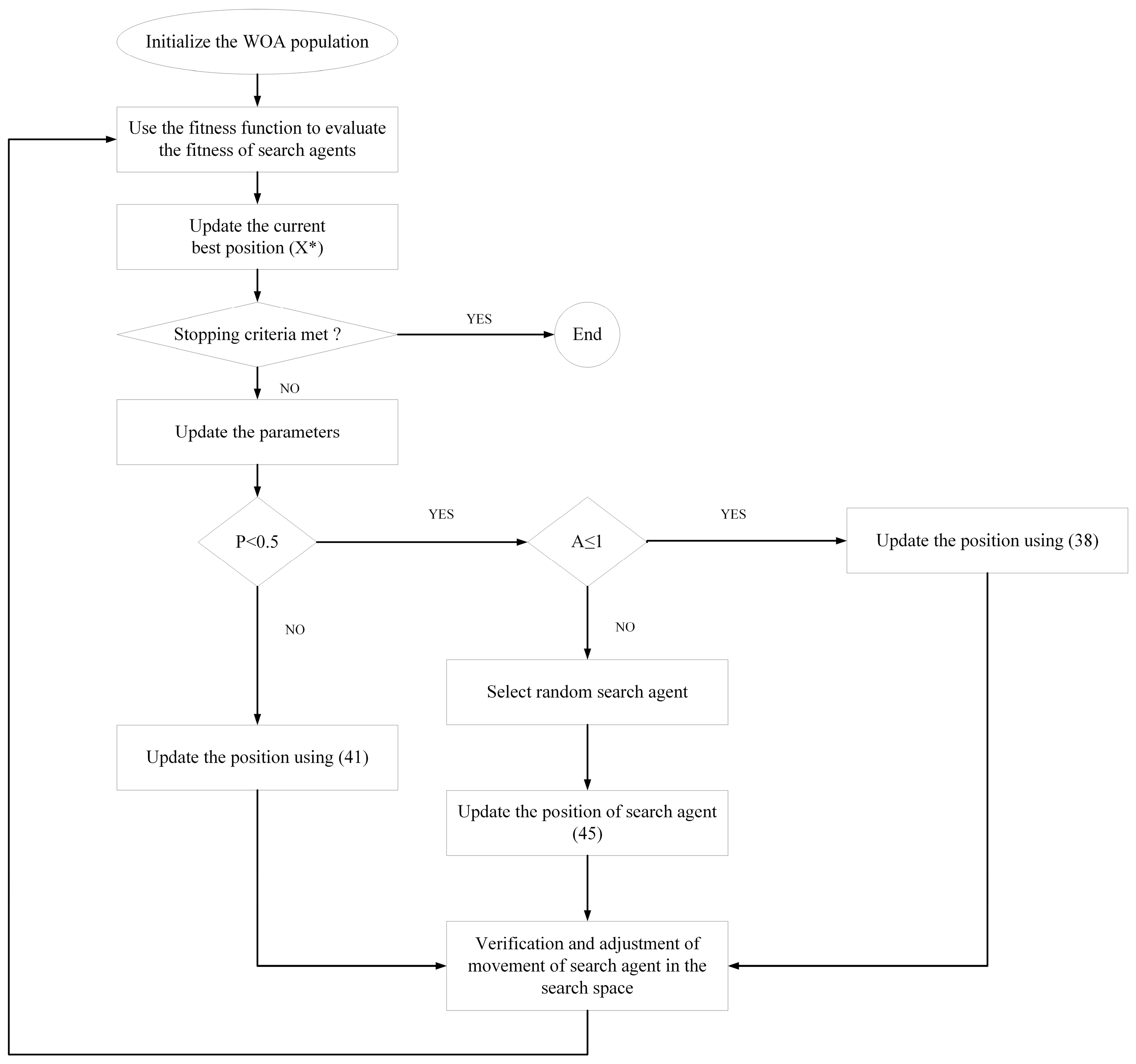
4.2.2. Whale Optimization Algorithm

The whale optimization algorithm (WOA) is inspired by the hunting behavior of humpback whales. The whale is one of the largest species of mammals and preys on small fishes. The humpback whale is one of the giant whales. Its working can be distinguished between the exploration and exploitation stages. The exploration stage is based on the bubble-net behavior of humpback whales. The mathematical function of this stage selects the spiral updating position and shrinking encircling mechanism.

Humpback whales detect their prey position and make a circle around them. As the optimal solution is not known a priori, the algorithm assumes that the current solution is an optimal solution. The remaining search agents adapt their positions according to the optimal solution. The positions of search agents and the position vectors are calculated using (41) and (42), respectively.

$$\overrightarrow{D}|\overrightarrow{c.}\overrightarrow{X^{*}}(t)-\overrightarrow{X}(t)|$$

(41)

$$\overrightarrow{X}(t+1)=\overrightarrow{X^{*}}(t)-\overrightarrow{A}.\overrightarrow{D}$$

(42)

where $\overrightarrow{D}$ = position of search agent, t = current iteration, $\overrightarrow{A}$,$\overrightarrow{C}$ = co-efficient vectors, $\overrightarrow{X^{*}}$ = position vector of current best solution, $\overrightarrow{X}$ = position vector. The relationships for co-efficient vector $\overrightarrow{A}$ and $\overrightarrow{C}$ are given as:

$$\overrightarrow{A}=2\overrightarrow{a}.\overrightarrow{r}-\overrightarrow{a}$$

(43)

$$\overrightarrow{C}=2.\overrightarrow{r}$$

(44)

$\overrightarrow{r}$ = random number (r $\in \left[0,1\right]$), $\overrightarrow{a}$ = linearly decreasing co-efficient between two and zero.

The updated position of search agent is between the current position and the current best candidate position. On the other hand, the spiral updating of position is based on following relationship:

$$\overrightarrow{X}(t+1)=\overrightarrow{D^t}.e^{bl}.\cos (2\pi l)+\overrightarrow{X^{*}}(t)$$

(45)

where $\overrightarrow{D^t}$ = distance between whale and the prey. This distance can be calculated at the ith iteration as:

$$\overrightarrow{D^t}=\left|X^{*}(t)-\overrightarrow{X}(t)\right|$$

(46)

B = constant for spiral shape, l = random number between [−1,1].

The whales in WOA circle around their prey in a shrinking manner and they also move along in a spiral shape. The probability that the whale uses encircling or spiral movement is not assumed apriori and it is tuned for considering the optimal performance. The flowing relationship is used for updating the position of whales considering their handling behavior:

$$\overrightarrow{X}(t+1)=\{{}_{\overrightarrow{D^t}.e^{bl}.\cos (2\pi l)+\overrightarrow{X^{*}}(t) \mathrm{if} p \ge 0.5}^{\overrightarrow{X^{*}}(t)-\overrightarrow{A}.\overrightarrow{D} \mathrm{if} p < 0.5}$$

(47)

Compared to the exploitation stage, a random search for the prey is performed by the whales in the exploration stage by tracing the position of each other. It helps the algorithm to perform a global search using the following relationship:

$$\overrightarrow{D}=\left|\overrightarrow{c.}\overrightarrow{X_{rand}}(t)-\overrightarrow{X}(t)\right|$$

(48)

$$\overrightarrow{X}(t+1)=\overrightarrow{X_{rand}}(t)-\overrightarrow{A}.\overrightarrow{D}$$

(49)

where $\overrightarrow{X_{rand}}$ is a random position vector.

During implementation, the algorithm creates an initial population of humpback whales. The flow chart of WOA algorithm is provided in Figure 4. The pseudo code of WOA is provided in our Appendix A (Figure A1). The main steps of WOA involve initiation, fitness value calculation and updating the position using the abovementioned relationships.

4.3. Hybrid NSGA-II and MOPSO

The purpose of hybridizing two algorithms is to extract and combine the positive aspects of either algorithm. Thus, it helps in solving complex problems more efficiently. Although a multitude of algorithms have been employed to solve complex problems, each approach is restricted by certain shortcomings. The aim of this section is to use a hybrid form of NSGA-II and MOPSO.

The non-sorting genetic algorithm (NSGA-II) is a non-domination based technique which is used for multi-objective analysis. The advantages offered by NSGA-II are improved sorting, no a priori requirement of sharing parameter and the inclusion of an elitism approach. NSGA-II has demonstrated an improved computational efficiency. The level of complexity it can undertake is defined by O (NP²) where N is the number of objectives and P represents the population size. It uses the following five operators: initializing, sorting, crossover, mutation and elitist comparison.

The particle swarm optimization (PSO) is a single objective based optimization algorithm. It is quite popular, due to its simplicity, use of relatively less parameters and an equal emphasis on local and global exploration. PSO is inspired by the behavior of birds flocking and fish schooling. During implementation, a bird is represented by a particle for single solution and the set of birds is represented by a swarm. During flight, each particle can be defined in terms of its position ($x_{ij}^t$) and velocity ($v_{ij}^t$). These are updated in each iteration of the algorithm.

The hybrid approach offers a compromise between exploration and exploitation. It divides the population into two halves. Once the ranking of non-dominated Pareto fronts is performed, the best half is used by NSGA-II while MOPSO uses the other half. The NSGA-II improves its half while MOPSO uses its half to converge them around the best possible solutions. Furthermore, the NSGA-II executes the exploration while exploitation is performed by MOPSO. The task of exploration helps the hybrid approach to reasonably assess the global solutions. The exploitation helps MOPSO to enhance the orientation of lower ranked particles towards a global solution.

It is to be noted that both approaches use different search techniques. For example, NSGA-II employs elitism and crowding distance sorting for attaining spread and diversity of Pareto optimal. On the other hand, MOPSO does not use the genetic operators and rather velocity and inertia weights are used to update the particle positions. Also, its parameters are constantly updated to escape local optima issues. The flowchart of hybrid NSGA-II MOPSO is given in Figure 5.

4.4. Parameter Tuning

The parameters of meta-heuristics are highly sensitive towards changes and thus they should be properly calibrated/tuned to ensure optimal performance. This section tunes the input parameters of ACO, WOA, NSGA-II and MOPSO. Three levels of input parameters were defined for each solution approach (

Table 1. Level of parameters for ACO.

Parameters	Level 1	Level 2	Level 3
Nu. of ants (m)	200	150	100
Nu. of iterations (NI)	200	300	400
Control parameter (Q)	100,000	200,000	300,000
Evaporation Rate (p)	0.3	0.5	0.7

,

Table 2. Level of parameters for WOA.

Parameters	Level 1	Level 2	Level 3
Number of whales (W)	100	200	300
Max. number of iterations (MI)	300	500	700
Probability of movement (pe)	0.4	0.5	0.6

,

Table 3. Level of parameters for NSGA-II.

Parameters	Level 1	Level 2	Level 3
Population size (pop size)	60	80	100
Number of iterations (Max. It)	600	800	1000
Crossover probability (pc)	0.2	0.4	0.6
Mutation probability (pm)	0.7	0.5	0.3

and

Table 4. Level of parameters for MOPSO.

Parameters	Level 1	Level 2	Level 3
Swarm size (P)	60	80	100
Maximum intertia (max. I)	0.9	0.7	0.5
Minimum inertia (min. I)	0.4	0.3	0.2
Maximum iterations (max. It)	600	800	1000

). A Taguchi design of experiment was conducted in Minitab V 19.2 to select optimal level of input parameters. Since no benchmark experiments were available in machine disruption based CLSC, a set of experiments was generated and each was run 10 times to obtain average values. Furthermore, since all objective functions were to be minimized, a smaller-the-better signal-to-noise (S/N) ratio approach was selected. The resulting main effect plots are provided in Figure 6. The optimal level values of input parameters were selected and they are provided in

Table 5. Optimal values of input parameters.

Algorithm	Set of Input Parameters	Optimal Values
ACO	(m, NI, Q, p)	(100, 400, 100,000, 0.5)
WOA	(W, MI, pe)	(300, 500, 0.6)
NSGA-II	(pop size, Max. it, pm, pc)	(100, 800, 0.4, 0.3)
MOPSO	(P, max. I, min. I, max. It )	(100, 0.9, 0.4, 1000)

.

Furthermore, in order to compare the performance of heuristics, we use the matrices of data envelopment analysis (DEA), mean ideal distance (MID) and computation time. The former two are desirable when their values are large while computation time is preferred to have a minimal value.

5. Data analysis and Results

5.1. Case Study

We used data related for a rubber tire manufacturing company in Pakistan to analyze the performance of various approaches and to implement the model. The company operates in the Punjab province of Pakistan and supplies locally manufactured tires to different customers and distribution centers. We selected the tire manufacturing company due to its extensive usage and environmental and health concerns. Recent reports indicate that more than 295 million tires are disposed of annually and about 20% of these tires are dumped in a way which harms the environment [46]. Also, the demand of tires increased by more than 4% in 2019 to a total number of around 3 billion worldwide [47].

The company produces tires for small vehicles (primarily cars) and we selected such a company due to the increased demand for cars and tires in Pakistan. The automotive industry is on the rise in Pakistan as it is becoming more affordable for each class in society due to the availability of financing through banks and other entities and the abundance of compressed natural gas (CNG) which is used as fuel. According to statistics, in Pakistan, over 11,900 cars were sold only in July 2020. Accordingly, the use and replacement of tires has also been increased in the recent years. The company aimed to reduce its overall cost, time and emissions by maximum recycling of the used tires instead of solely relying on the supplier for raw material.

The supply chain of the selected case study considers single supplier, multiple distribution points, multiple customers and a single repository for return for the case of a single product of car tires. The company uses steel wire and rubber powder as a raw material for tire manufacturing. The finished products are supplied to local distribution centers which are used to deliver the products to end users. The returned tires lot is inspected and sorted at the repository. This helps the management in selecting the repairable tires. There are a number of available machines to repair/re-manufacture the tires and the retread tires are supplied to the secondary market. The remaining tires are sent to a tertiary market where they are evaluated against the feasible options of energy extraction and land filling, etc.

The company archives provided details on supply to variable distribution centers and a number of customers using different sets of machine facilities. For experimentation purposes, we divided the archived and current supply chain data into different problem sizes (small, medium and large). The relevant data is provided in

Table 6. Different problem sizes and their associated data.

Problem Size	Test Problem	Machine Facilities	Distributors	Customers
Small	1	2	2	4
	2	4	4	6
	3	5	5	8
Medium	4	10	8	10
	5	15	8	15
	6	20	10	20
Large	7	40	12	30
	8	50	14	40
	9	60	16	45
	10	70	20	55

which contains distribution points varying between 2 to 20 centers for 4 to 55 classes of customers.

The production capacity of each machine facility is restricted to 1000 units/machine. For each test instance, the concerned data of machine disruption varies. As an example, we provide the machine data related to the 4th test problem (10 machine facilities) in

Table 7. Machine related data of Test problem 4.

	Machine	Capacity		Cost				Time
		Facj	Ncaj	cej	cj	cwj	rwj	tpj	ttj	trmj
Test Problem 4	M1	75	25	500	165	180	45	25	12	18
	M2	60	40	400	150	200	38	22	11	16
	M3	80	20	575	180	325	55	29	14	18
	M4	68	32	365	155	145	35	24	12	15
	M5	72	28	460	170	170	48	27	13	15
	M6	70	30	445	165	185	50	32	17	16
	M7	65	35	400	130	135	45	23	14	15
	M8	62	38	430	145	130	55	20	12	13
	M9	75	25	485	160	190	65	32	18	15
	M10	83	17	600	195	345	65	38	20	17

. The capacity of production (feasible and non-feasible) is in unit of production and cost and time data are given in USD and minute, respectively. The CLSC is designed to meet the required demand quantity of 10,000 units of tires.

5.2. Results

The approaches were implemented in LINGO 14.0 and Matlab 2014a (for $\epsilon$-constraint method) and Matlab 2014a for meta-heuristics and hybrid algorithms. A system with specifications Intel Core i5, 8th generation with 8 GB RAM was used for different procedures. Initially, a set of problems was tested and their computation time was noted against each problem size. Figure 7 displays the results of computational time (CPU) of various approaches. The analysis was repeated 10 times in order to gain statistical confidence. As can be seen, $\epsilon$-constraint is an ideal approach for small problem sizes (1–3) and it takes less time to solve the problem. For medium and large problems, hybrid NSGA-II-MOPSO takes relatively less time followed by WOA and ACO.

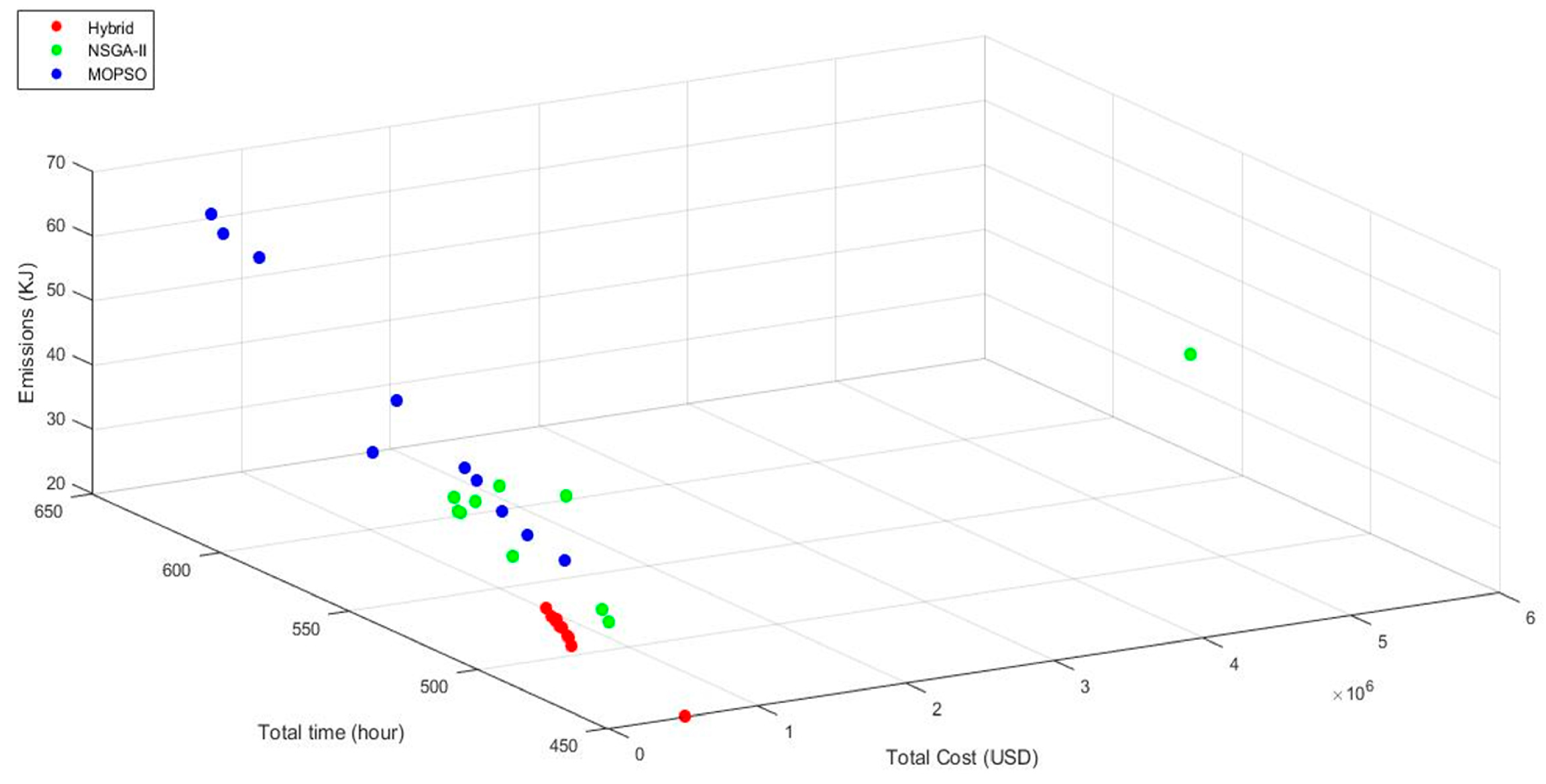
Algorithms in the hybrid approach are based on non-domination of Pareto optimal solutions. We tested results of the hybrid approach in comparison with NSGA-II and MOPSO. The test problem 7 was used for the analysis and top 10 Pareto Fronts (PF) for each approach are plotted in Figure 8. The analysis was re-iterated 10 times for statistical purposes. As can be observed, more solutions of hybrid approach are closer to origin. In other words, the hybrid approach offers more choices of optimal candidate solutions, which is primarily due to the merger of the external archive and repository of NSGA-II and MOPSO, respectively. The division of population in the hybrid approach helps in mitigating a pre-mature convergence and refinement to achieve more optimal solutions. NSGA-II solutions are somewhere between the hybrid and MOPSO solutions. In comparison, the solutions of MOPSO show more deviation and provides less solutions for the choice of optimal PFs.

In order to evaluate the performance of each algorithm against the used matrices, a relative deviation index (DI) measure was used. A smaller value of DI is preferred and it is given by (50) as:

$$relative deviation index (DI)=\frac{A_{sol}-B_{sol}}{M_{sol}-Mi{n}_{sol}}\times 100$$

(50)

where A_sol = value obtained by the algorithm, M_sol = max. value of performance measure, Min_sol = minimum value of performance measure, B_sol = best solution among the algorithms. The DI was calculated using the interval plot in Minitab V 19.2 and respective results are provided in Figure 9. It can be observed that in all sub-figures (Figure 9a–d), there is no statistical difference in the performance of NSGA-II and MOPSO. The hybrid approach is more robust in terms of DEA, MID and CPU. Also, compared to ACO, WOA performs well in terms of DEA, MID and CPU matrices. Lastly, an increasing shift of deviation is observed in all approaches when problem size is increased from medium to large scale.

The literature suggests that the probability of mutation in the hybrid algorithm affects the population. To demonstrate this, a sensitivity analysis of different mutation values was performed, and the results are displayed in Figure 10. The plot is provided between the number of iterations and population percentage. It can be observed that the mutation values affect the population i.e., higher the rate of mutation, a large number of iterations are taken to diminish the effect of mutation rate on the population. For instance, for m = 0.1, the algorithm does not affect the population beyond 95 iterations while m = 0.4 needs 255 iterations to diminish the effect on the population.

Similarly, we analyzed the effect of combination of crossover and mutation values in NSGA-II on the convergence of solution. The results are plotted for different problem sizes in Figure 11. The value of m = 0.6 refers to mutation probability value = 0.6 and crossover probability value = 0.4. It can be observed that as the problem size increases and the mutation probability value decreases, the convergence decreases. It can be argued that a higher value of mutation probability is needed for higher convergence. The convergence affects the quantity of Pareto optimal solutions i.e.; higher convergence warrants an increased number of Pareto optimal solutions.

Sensitivity Analysis

In this study, beside other aspects, we analyzed machine disruption and total time of a CLSC network. We analyzed the effect of changing values of disruption probability on LT, RT, RC, FC and NM and the respective results are provided in Figure 12. It can be observed that by increasing the probability of disruption, re-work cost and time (RC and RT) increases. This is because more products fail and are discarded due to higher disruption, and hence less quantity is available for re-working. On the other hand, by increasing the probability value, an increase in the percentage of FC, LT and NM is observed. It means that higher disruption leads to more failed units and hence an increase in the number of machines (NM) to compensate for the failed units. Similarly, more failed units lead to higher failed units cost (FC) and more production time (LT). These graphs can provide valuable insights to managers for a trade-off analysis. For example, as disruption increases, the re-work cost (RC) decreases while the failed cost (FC) increases and a trade-off is achieved between them at ${\lambda }_j$ = 0.47. Similarly, a trade-off can be achieved between lost time (LT) and re-work time (RT) at ${\lambda }_j$ = 0.52.

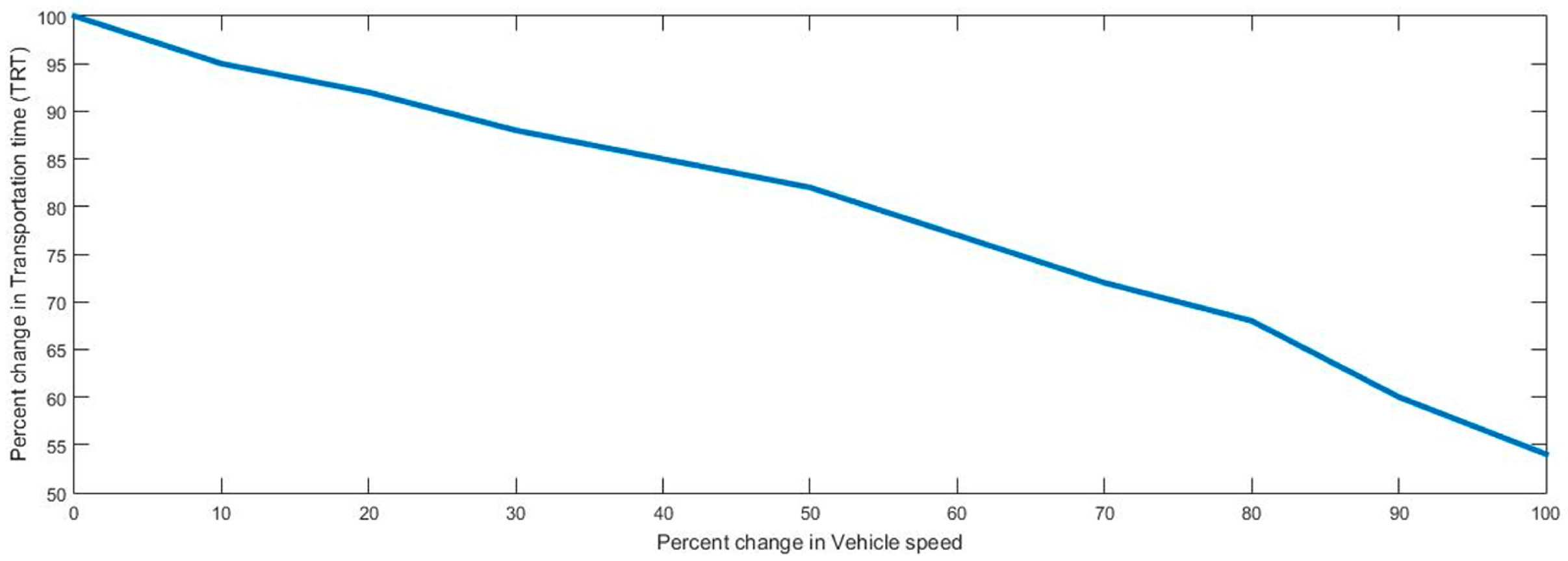
The effect of an increase in vehicle speed on the total transportation time (TRT) was analyzed, and the respective results are provided in Figure 13. By doubling the vehicle speed (i.e.; 100% increase), the TRT can be approximately reduced by 45%. The managers can increase the vehicle speed to achieve better results, however, its effect on the emissions and carbon footprints can be alarming.

We used different combinations of disruptive machines of test problem 4 (Table 7) and analyzed the variation in different objective functions. In order to do so, we relaxed Equation (17) (which requires the production using only one machine) and re-analyzed the problem. The relevant results are provided in Figure 14. For a cost sensitive CLSC network, manufacturing system can use minimum number of machines (set 3), however, a long queue of products will be resulted due to the availability of less machines which will elevate the total time. Similarly, due to limited options of machines, the manufacturing plant will not be able to shift the products from more disruptive to relatively stable machines. This will result in an increased emission due to machine disruption. On the other hand, by using more machines (set 5), the manufacturing plant can divide the work to minimize the total time at the expense of additional cost. Also, it will have the opportunity to control the emissions by shifting the work to other machines.

To summarize, the CLSC primarily focuses on an outward looking approach where efficiency of the network is maximized by optimizing transportation, using carbon cap policy and analyzing supplier competition. For example, performance enhancement through cost and efficiency analysis [10], incentive plans for retrieving different quality products [11], environmental analysis [12,16] and analyzing the disruptions in demand [48] are some of the relevant cases. Compared to these studies, we have embedded an inward looking approach by analyzing the impact of machine disruptions on overall efficiency of the CLSC network.

5.3. Managerial Implications

CLSC is normally considered an outward looking approach for dealing with buyer and suppliers and their associated disturbances, however, our findings have shown the impact of in-house disruption in production on the overall efficiency of CLSC network. We have the following implications which are not only applicable to the tire industry but they can also be applied to the supply chain of any good industry.

The objective of cost, time and emission are in conflict with each other; however, an efficient CLSC of tire manufacturing industry can be designed by controlling the emissions (Figure 8). In other words, cost and time savings can be achieved by reducing the overall emissions.

The manufacturing system agreed that besides other aspects, emissions can be controlled by using an adequate number of machines and devising an efficient transportation mechanism. We shared the optimal OBV values i.e., TC = 700,000 USD, TT = 451 hours and CE = 21.3 KJ with the industry and these values were compared with their baseline data. On average, our results proved to be more than 16% effective as our analysis pointed out which machines, distribution centers and potential customer locations to choose in the CLSC network.

When less machines are used, the manufacturing plant will have a tighter transportation mechanism to deliver the products responsively. This might necessitate a faster speed of delivery which will further add to the overall emissions. When more machines are used for production, the manufacturing plant will be able to complete demand before the due date. This will provide an opportunity to complete any backorders to take maximum advantage of the available machine facilities. Also, a normal delivery will take place which can also help in controlling the emissions.

The managers can consider the following operation rule for controlling the in-house waste. For low to moderate disruption of machine, the product demand can be accomplished with the use of 10% less machines. Doing so will help accomplishing remarkable cost and time saving and less emissions. The tire transportation can be accomplished by using an increased vehicle speed, however, it might require efficient driving skills.

Our current observation of the archived data informs that the failed units are discarded which are taken away by local villagers. These tires are used for storing ice and carrying water in far flung areas. It is to be noted that the water filled tires are a hotspot for mosquitoes and such practices increase the chances of spread of Dengue virus [49], especially in the Punjab province of Pakistan. Since the failed units of tires due to machine disruption are discarded, it is recommended to use them in other areas of application. Such as, they can be used in the sports fields, making shoes and paving the roads.

6. Conclusions and Suggestions for Future Research

This study analyzed a CLSC supply chain using the objectives of cost, time and emissions. To the best of our knowledge, this is a first attempt to analyze the machine disruption and total time of the network. Different solution approaches were implemented on test problems and a detailed analysis was presented regarding the aspects of solution approaches and the presented model. The findings highlight the impact of machine disruption on the trade-off analysis of different decision variables and the effect of input parameters on the performance of solution approaches. In particular, the results reported that for a different set of disruptive machines, the objective function values varied. For instance, when more machines are employed, the total cost goes up; however, the demand is fulfilled using less time and less emissions and vice versa. The trade-off between different choices will help the practitioners select the appropriate set of machines when facing delivery schedules and meeting back-orders. The literature weighs more on out-of-production entities in the CLSC network design. Our findings provide an inward looking approach and will help practitioners to emphasize on the role of production and machine selection on the supply chain performance.

This study contains certain limitations. Firstly, we analyzed a deterministic model without considering dynamic behavior of the CLSC. Secondly, a single supplier was used and hence there was no competition among the suppliers. Thirdly, although inspection was used, its impact was not considered in the analysis. It was assumed that inspection does not incur any cost.

We provide the following recommendations for future research. Currently, we analyzed the case of a single product while modern supply chains are focusing on multiple products [50]. Thus, future research can aim at the integration of different products in a multiple supplier, cross-docks and multiple markets of a closed loop supply chain. The presented analysis can be extended by analyzing the stochastic behavior of input parameters. For example, in industrial settings, the disruptive profile of machine is usually non-deterministic. Thus, including the fuzzy nature of such variables can bring the implications much closer to reality. Also, competitiveness in the supply chain is gaining more popularity. Such competition exists either among multiple suppliers, multiple manufacturing system or among supplier and manufacturing system. Game theory and Nash equilibrium approaches can be used for analyzing such competitive closed loop supply chains. Lastly, this study was a first attempt towards the hybridization of powerful meta-heuristics (such as, NSGA-II and MOPSO) in the context of CLSC networks. This generic framework can be applied to different case studies, as well as compared with other hybrid heuristics. Also, the findings of the algorithms can be compared with other solution approaches such as archived multi-objective simulated annealing and bees’ algorithm for optimal performance.