An Integrated Procedure for Ex-Ante Evaluations of Refurbishment Costs in Healthcare Facilities

Abstract

This paper focuses on the valuation of refurbishment costs for healthcare facilities. The determination of the more reliable approach for experimental verification is a research topic of great interest, especially because previous literature on the matter is limited. This study examines ex-ante cost valuations in the refurbishment of healthcare buildings while using similarity to estimate the costs that are based on the amount of already accomplished renovations. The methodology involved a desk analysis deter-mining the technical valuation of intervention needs, and similarity coefficient applications providing a refurbishment cost valuation. The application was conducted in the Friuli—Venezia Giulia Region in Italy, where hospitals show structural, layout, and plants deficits with respect to current regulations, and a technical deepening to identify critical issues is required to prepare a multi-year intervention plan. The case study results showed that this procedure requires little initial information to run analyses and its application can support investment budget planning purposes.

1. Introduction

Construction cost ex-ante evaluations is a topic of great practical interest for both the private and public sectors, as a cost estimate is the starting point for any convenience evaluation. For private operators, the construction cost is essential for estimating the expected profit, while, for public operators, it is essential for efficient public financial resource allocations. Normally, a building’s construction cost can be estimated through (1) an analytical-reconstructive procedure, which, starting from the detailed building project, identifies the necessary elementary work entities and calculates the total construction cost, or (2) a synthetic-comparative process that identifies the construction market’s costs and compares the chosen building with similar buildings to estimate the costs. Although the first procedure has the advantage of considering all of the building’s peculiarities, it requires a detailed project and does not consider the discounts usually offered by construction companies. This is aimed at determining the order of magnitude of the monetary amount of the construction cost of the workings [1]. The second procedure begins with a brief description of the needed work and, based on the actual incurred costs for similar buildings, embeds the most probable rebates and contingencies. It is usually used to determine the order of magnitude of the budget [1]. In other words, the analytical procedure does not take into account the uncertainties of establishing contracts and completing the building, while the synthetic procedure is based on a less precise building description. As such, determining which approach is more reliable for experimental verification is a research topic of great interest, especially because previous literature on the matter is limited. The synthetic-comparative approach can produce an ex-ante valuation of the construction cost based on this description, as the executive design is not yet available. Moreover, only this approach can be used when the cost estimate aims to support the planning of a multi-annual investment budget. There are several studies that provide parametric costs that can be useful for synthetic estimates of retrofitting intervention. Among these, we mention those proposed by Di Ludovico et al. [2], which focus on reconstructions following seismic events, and Dell’Anna et al. [3], which focused on the energy requalification of residential buildings. The synthetic cost estimation procedures are also used in the evaluation of the benefits that derive from seismic retrofit and integrated seismic and energy interventions [4,5].

The appraisal discipline has developed various approaches in the last century to effectively compare the value of goods with similar, but not identical, characteristics. In appraisal theory, Jev-ons’s law of indifference can produce the most probable market or production value estimation: ‘when a commodity is perfectly uniform or homogeneous in quality, any portion may be indifferently used in place of an equal portion: hence, in the same market, and at the same moment, all portions must be exchanged at the same ratio’ [6]. In other words, they have the same value. The law of indifference is very intuitive and easily applicable when the commodity market is competitive, as the subject characteristics are then identical to those of the goods with known price. However, when the goods are not homogeneous, the application becomes more problematic. In these cases, it is necessary to adopt one or more comparison criteria capable of incorporating the differences between the chosen good and similar ones for which the cost is known.

The methodology has been developed referring the valuation of intervention costs for healthcare facilities in the Friuli-Venezia Giulia region, in the north-east of Italy. Many of these hospitals show structural, layout, and plants deficits with respect to current regulations. This methodology attempts to resolve this relevant problem. Moreover, the Regional Administration has begun a technical deepening on the existing facilities in order to identify the critical issues and prepare a multi-year intervention plan.

Although the concept of similarity is pervasive in appraisal, there are few published contributions that propose similarity measures as a comparison method for assessing an evaluated object and similar objects of known value. Further, to our knowledge, similarity measures have never been used for the appraisal of building construction and refurbishment costs. Thus, in this study, we explore the possibility of applying the law of indifference for a cost ex-ante valuation of building refurbishment interventions. In other words, as we know the renovation costs for the existing buildings (comparable elements), we attempt to estimate the cost of refurbishing a healthcare building based on its similarities with the comparable elements, while using an evaluation model that adopts qualitative and quantitative similarity coefficients. We hypothesize that we can estimate the cost from similar intervention costs, and that the degree of similarity between the intervention itself and similar ones represents the weights that the latter assumes in the assessment. Using the same parameters as the similarity inquiry, we will also provide a quick method for the technical assessment of refurbishment needs through a desk analysis determining the building units and technical systems that are in need of refurbishment.

2. An Overview of Similarity Coefficients

Similarity coefficients are normally used to solve assignment, classification, and/or clustering problems in various fields [7,8], such as biology [9,10], ethnology [11], taxonomy [12], image retrieval [13], geology [14], chemistry [15], and ecology [16,17,18]. Similarity and its inverse distance measures can be classified in various ways according to the data used in qualitative, semi-quantitative, and quantitative studies. Similarity coefficients, which are usually devoted to qualitative data, provide a measure of analogy degrees between 0 and 1. Qualitative similarity measures are based on the qualities present in the considered objects. Obviously, the greater the number of similar qualities, the greater the degree of similarity.

Another important element in the classification of similarity measures concerns the used information’s degree of completeness in the measure calculations. In fact, the absence of a certain quality can signify certainly absent or a lack of information on that specific characteristic. In this regard, it is useful to distinguish between the symmetrical and asymmetrical similarity measures. Thus, a distinction must be made between sure and missing data when the information is incomplete. Symmetric measures consider absence as certain data, while asymmetric ones consider it as lack of information. In these different cases, one would choose symmetric similarity coefficients and asymmetric similarity coefficients, respectively.

2.1. Qualitative Similarity Coefficients

Qualitative similarity coefficients normally adopt a binary coding of the information that is used to calculate the similarity degree. For example, if we consider two objects, j and k, and assume x_i characteristics, with i = n and where x_i is 1, the object has the i-th characteristic; otherwise, it is 0. In symmetric coefficients, the value 0 represents the sure absence of the feature.

Table 1. Scheme for symmetric and asymmetric similarity coefficients.

Object k	Object j
	1	0
1	a	b
0	c	d

summarizes the two objects comparison with respect to the x_i characteristics:

a:

number of qualities present in both objects

d:

number of qualities absent in both objects

b:

number of qualities present in object k and absent in object j

c:

number of qualities present in object j and absent in object k.

In the symmetric coefficients, if we assume that the x_i characteristics completely describe the objects, then the present (1/1: a) and absent (0/0: d) qualities in both objects express their degree of similarity. The most common symmetric coefficients are calculated from the ratio between the number of coincident descriptors (a + d) and the total number of descriptors n. However, they are distinguished by the different weight attributed to the concordant and discordant descriptors.

The simple matching coefficient (1) does not discern between 0 and 1 and it is given by the simple ratio between the number of descriptors with the same value (a, d) and the total number of descriptors (n) [12]. The Rogers & Tanimoto coefficient (2), a variant of the previous one that doubles the weight of discordances (b, c), considers more similar observations with fewer discordances [19]. Finally, the Sneath & Sokal coefficient (3) is a further variant of the previous coefficients, as it is conceptually opposite, because it gives a double weight to the concordances (a, d) and considers more similar observations with the largest number of concordances [20].

$$\mathrm{Simple}\mathrm{Marching}{S}_{jk}=\frac{a+d}{a+b+c+d}$$

(1)

$$\mathrm{Rogers}\&\mathrm{Tanimoto}{S}_{jk}=\frac{a+d}{a+2b+2c+d}$$

(2)

$$\mathrm{Sneath}\&\mathrm{Sokal} S_{jk}=\frac{2a+2d}{2a+b+c+2d}$$

(3)

The asymmetric similarity coefficients, as mentioned above, consider the absence of a characteristic as a lack of information. In other words, this method does not exclude the possibility that the characteristic is present. In this case, the various coefficients are calculated from the ratio between the number of features that are present in both objects (a) and the number of characteristics certainly in agreement (a) added to the discordant ones (b, c). Among the asymmetric coefficients, the Jaccard coefficient (S4) is strikingly similar to the simple matching coefficient, but it does not consider the discordances (d) and it represents the ratio between the concordances and the number of non-zero values [21]. The Sørensen coefficient (5) gives double weight to the concordances, emphasizing the asymmetric criterion [22]. The last two coefficients are used in data samples with uncertain representativeness due to a lack of information.

$$\mathrm{Jaccard}{S}_{jk}=\frac{a}{a+b+c}$$

(4)

$$\mathrm{Sørensen}{S}_{jk}=\frac{2a}{2a+b+c}$$

(5)

2.2. Semi-Quantitative and Quantitative Similarity Coefficients

Semi-quantitative and quantitative similarity coefficients are used when the ordinal or cardinal variables describe the compared objects. The quantitative coefficients are distinguished from the qualitative ones to consider not only the presence or absence of a given characteristic, but also its size. For this reason, they are an interesting method to evaluate similarity with respect to the characteristics that influence the market value or production costs.

The Steinhaus coefficient [23], Rudjichka coefficient [24], and Kulczynski coefficient [25] propose similarity measures, starting from a summation of the minimum values found in the compared objects, but they adopt different normalization procedures.

The Steinhaus coefficient (6) normalizes for the summation of the descriptor values, while the Rudjichka coefficient (7) normalizes for the maximum value of each descriptor. Finally, the Kulczynski coefficient (8) represents the ratio between the summation of the minimum values recorded in the two objects’ descriptors and their respective summations.

The quantitative Jaccard coefficient [21], also known as the Tanimoto coefficient [26], the Dice coefficient [27], and the Cosine coefficient, instead, propose similarity coefficients, starting from the summations of the products between each descriptor. Jaccard (9) normalizes the product by summing the squares of the product’s diminished descriptors. Dice (10) normalizes the product’s double among the descriptors with the sum of the descriptors’ squares. Finally, the Cosine measure (11) normalizes the product between the descriptors with the summation’s square roots of each descriptor’s squares.

$$\mathrm{Steinhaus}{S}_{jk}=\frac{2{\sum }_{i=1}^n\min (x_{ij},x_{ik})}{{\sum }_{i=1}^n{x}_{ij}+x_{ik}}$$

(6)

$$\mathrm{Rudjichka}{S}_{jk}=\frac{{\sum }_{i=1}^n\min (x_{ij},x_{ik})}{{\sum }_{i=1}^n{x}_{ij}+x_{ik}}$$

(7)

$$\mathrm{Kulczynski}{S}_{jk}=\frac{1}{2}\left[\frac{{\sum }_{i=1}^n\min (x_{ij},x_{ik})}{{\sum }_{i=1}^n{x}_{ij}}+\frac{{\sum }_{i=1}^n\min (x_{ij},x_{ik})}{{\sum }_{i=1}^n{x}_{ik}}\right]$$

(8)

$$\mathrm{Jaccard}{S}_{jk}=\frac{{\sum }_{i=1}^n{x}_{ij}{x}_{ik}}{{\sum }_{i=1}^n{x}_{ij}{}^2+{\sum }_{i=1}^n{x}_{ik}{}^2-{\sum }_{i=1}^n{x}_{ij}{x}_{ik}}$$

(9)

$$\mathrm{Dice}{S}_{jk}=\frac{2{\sum }_{i=1}^n{x}_{ij}{x}_{ik}}{{\sum }_{i=1}^n{x}_{ij}{}^2+{\sum }_{i=1}^n{x}_{ik}{}^2}$$

(10)

$$\mathrm{Cosine}{S}_{jk}=\frac{{\sum }_{i=1}^n{x}_{ij}{x}_{ik}}{\sqrt{{\sum }_{i=1}^n{x}_{ij}{}^2}\sqrt{{\sum }_{i=1}^n{x}_{ik}{}^2}}$$

(11)

3. Current Applications of Similarity Coefficients

Most of the existing literature proposes examining similarity for the selection of comparable items or to implement the adjustment grid method. Isakson [28] developed the Nearest Neighbours Appraisal Technique (NNAT) as both an improvement of, and an alternative to, adjustment grid methods for house value estimations. Supposing that all of the properties in a particular market are rank-ordered by value, the subject property’s value can be expressed, as in Equation (12), where the weights represent the nearness/similarity of the subject to the comparable properties. The weight associated with each comparable item is calculated, starting from the inverse of the Malahanobis distance [29], which allows for the method to consider, in the similarity’s estimation, the presence of correlations among the descriptors. In further applications on different properties (dwelling building, industrial properties, office buildings, and retail, etc.), Isakson [30] pitted the NNAT against the traditional real estate appraisal process and the ordinary least square (OLS). The results showed that the NNAT was significantly more accurate than the other two estimates for retail and other miscellaneous properties, but not for other property types.

$$\widehat{P_i}={\sum }_{j=1}^k{W}_{ij}{P}_j\mathrm{with}{w}_{ij}=\frac{\left(\raisebox{1ex}{$1$}\!\left/ \!\raisebox{-1ex}{${\mathrm{D}}_{ij}^2$}\right.\right)}{{\sum }_{i=1}^k\left(\raisebox{1ex}{$1$}\!\left/ \!\raisebox{-1ex}{${\mathrm{D}}_{ij}^2$}\right.\right)}$$

(12)

where

$\widehat{P_i}$ is the expected price the of house,

$P_j$is actual the price of the house j,

$W_{ij}$is the nearness of house j to house i,

$k$ is the number of comparable items,

$D_{ij}$ is the Mahalanobis distance between property i and j.

Other studies assessed the comparable sample’s similarity and reliability degrees in the market-oriented appraisal method, particularly the Market Comparison Approach (MCA) [31,32,33,34]. These studies introduced two different similarity coefficients, a reliability coefficient and two second level indexes, which combine similarity and reliability measures. The similarity indexes are calculated with respect to the differences between the considered objects’ descriptors, while the reliability coefficient is calculated, instead, based on the differences in the correct prices. These studies propose the adoption of these indexes in MCA’s reconciliation phase if the corrected price diverge. In particular, they suggest weighting the corrected prices with (i) similarity coefficients if the divergence of the corrected price is related to real estate characteristics, (ii) reliability coefficients if the divergence is related to market prices, or (iii) second level indexes if the divergence is related to both real estate characteristics and market prices.

Kulczycki and Ligas [35] presented a procedure for assessing the similarities between properties when they are described by qualitative attributes. They used a computational procedure to transform a nominal attribute into a corresponding set of dummy binary attributes. Subsequently, they applied different similarity coefficients for qualitative data and compared the results by ranking and grouping the sample properties that were derived from different coefficients. Finally, they determined the best similarity coefficients for real estate market application.

Zyga deepened the relationship between estimate validity and comparable item similarities, showing that estimated prices using statistical approaches often ‘do not always meet the requirements of statutory definition of market value’ [36]. Moreover, the author stressed the need to apply statistical approaches to similarly preselected data sets with the object of the estimate, because ‘for the purpose of real estate appraisal itself, the selection of data is more useful than searching for a price model’ [37].

This review shows how, for estimative purposes, incorporating similarity in the evaluation process is fundamental for obtaining good estimates, even in the presence of limited market data. In fact, in the presence of limited random data, statistical approaches are not usable, and mathematical attempts often provide results that contrast the market evidence. For similarity analysis, using a comparison criterion or refining an estimate for MCA can be a useful support tool. The above considerations essentially concern evaluations of building market values, but they can easily be extended to examining construction costs, as this also represents a value that is formed in a market.

4. Materials and Methods

Ex-ante evaluation of a healthcare building’s refurbishment costs is important for the administration of public finances, as health spending represents 9.8% of the GDP in European Union countries and 75% of it is financed by member states [38]. Furthermore, old buildings with significant structural, energy, and plant deficits require urgent and expensive redevelopment [39]. Therefore, the ability to forecast refurbishment expenditures is of great importance to efficiently plan budgetary commitments. This need is even greater in areas at risk of earthquakes, where it is necessary to guarantee the full functionality of health facilities, especially first aid facilities.

The operational phase implies performing maintenance and refurbishments on built heritage sites due to progressive performance lacks. Thus, building asset management becomes increasingly complicated and requires specific knowledge [40]. In healthcare facilities, building conditions are a challenging task involving data acquisition and performance assessments due to their physical systems, special plants, and diverse functional spaces [41].

In the present research, implementing a technical evaluation of the current building status is crucial, as budget estimation in the refurbishment of a healthcare building requires a quick method to assess building conditions based on relevant key performance indicators [42]. This method, applied by a competent assessor, does not replace the analytic-reconstructive procedure that prepares a detailed project. However, it provides asset managers and decision-makers a lean tool for investigating building conditions and activating appropriate interventions based on visual inspections and document availabilities [43].

The proposed methodology investigates a healthcare facility built in a heritage building and considers the criteria that drive refurbishment, adjustment, and modernization policies for large healthcare facilities [44]. The evaluation methodology aims to achieve two targets:

A.

identifying the intervention needs of the considered healthcare context (subject) that has deteriorated according to the standards. These interventions can identify the areas in which it will be necessary to operate to refurbish the subject (Technical Assessment); and,

B.

estimating the costs of the subject’s refurbishments, made possible by the performance data derived from the first phase (Economic Valuation).

Specifically, we performed the valuation of intervention costs for health facilities in the Friuli–Venezia Giulia region, in north-eastern Italy. Many of these hospitals have structural, layout, and plants deficits with respect to current regulations. Thus, the Regional Administration has begun focusing on the existing facilities in order to identify the critical issues and prepare a multi-year intervention plan.

4.1. Technical Assessment

To achieve target A and the research purpose, we developed a Quick Requirement Assessment (QRA) method that can be broken down into the following phases:

• Assessing refurbishment needs.
• Defining the appropriate Standard Interventions (SI).
• Identifying intervention needs through the activation of one or more SIs.

The assessment involves both documentation study and non-invasive evaluations, and it contains a Quick Subject Survey (QSS), a Standard Intervention Definition (SID), and a Quick Technical Evaluation (QTE) (Figure 1). The QRA procedure is based on the hypothesis that a hospital, a structure of the highest complexity, requires a very high maintenance level that is constantly performed according to advanced commissioning standards. Consequently, the QRA assumes that the building construction or extraordinary repairs/refurbishments/re-developments of its subsystems have achieved a verified level of regulatory compliance. The complexities and extent of the envisioned verifications for the accreditation of hospitals justify this hypothesis.

4.1.1. QSS (Subroutine A.1)

According to the QRA’s hypothesis, it is possible to achieve a quick evaluation of the subject’s intervention needs. Experienced personnel that have access to the technical documentation behind the subject’s construction and total interventions can perform this first subroutine (QSS). The QSS consists of three steps, coded as QSS.1, QSS.2, and QSS.3, and it represents the collection of technical information: subject history reconstruction, site condition evaluations, and integrative technical findings.

The first step, QSS.1, aims to overview the subject’s history, highlighting its construction period and all significant interventions concerning its technological systems, given the importance of key hospital equipment [41].

Table 2. Section QSS.1: documented history.

QSS—Section QSS.1
Features	Possible Options
	1	2	3	4	5	6
QSS.1.1. Construction period	<1900	1901–1938	1939–1967	1968–1996	1997–2000	>2000
QSS.1.2. Latest interventions in structural adjustments/improvements	<1975	1975–1986	1987–1996	1997–2003	2004–2008	>2009
QSS.1.3. Latest energy refurbishments of opaque envelope	<1976	1977–1991	1992–2005	2006–2015	>2015	-
QSS.1.4. Latest energy refurbishment of transparent envelope	<1976	1977–1991	1992–2005	2006–2015	>2015	-
QSS.1.5. Installation period or latest requalification of HVAC systems and plants	<1991	1992–2005	2006–2011	2012–2015	>2015	-
QSS.1.6. Installation period or latest requalification of fire-extinguishing and fire-detection plants	<1984	1985–2002	2003–2012	2013–2015	>2015	-
QSS.1.7. Installation period or latest requalification of special and electric plants	<1971	1971–1990	1991–2008	>2008	-	-
QSS.1.8. Installation period or latest requalification of elevators and lift systems	<1997	1997–2005	2006–2017	>2017	-	-
QSS.1.9. Installation period or latest requalification of medical gas plants	<1997	1997–2010	2010–2017	>2017	-	-
QSS.1.10. Latest intervention for layout adjustments/architectural barrier removals	<1978	1978–1996	>1996	-	-	-
QSS.1.11. Latest interventions adjusting the infrastructures for contaminated waste disposal and waste storage areas	<1996	1997–2006	>2007	-	-	-

lists the significant features that essentially describe the subject through the time periods representing the typological and technological evolutions of hospitals. QSS.1.1 offers the significant dates in which technological developments and regulatory updates had an impact on the hospital’s design in the Italian context [45,46,47,48].

We determined up to six possible options for each feature QSS.1.2–QSS.1.11, as it is essential to identify the most recent interventions on the subject’s spatial and technological systems. Every option refers to the issues of legislative regulations that updated design criteria, and a technological system’s implementation and management. It is reasonable to assume that these regulations have driven previous interventions for refurbishment, maintenance, and adaptation. The considered features involve the following:

• structural adjustments and improvements [49,50,51,52,53];
• building envelope refurbishments [54,55,56,57];
• HVAC system installations and requalifications [55,56,57,58];
• fire-detection system installations and adjustments [59,60,61,62];
• electrical and special equipment installations and requalifications [63,64,65];
• renovation and enhancement of lifting plants and facilities [66,67];
• renovation and enhancement of medical gas plants [68,69];
• indoor layout renovations and adjustments, and architectural barrier removals [70,71]; and,
• sanitary waste treatment and storage area improvements [72,73,74,75].

For each feature, we assigned a value between a variable range to each option. The options are valued in accordance with their maximum number (Table 2). A more recent refurbishment/improvement/adjustment intervention assigns a higher value to the feature and this value increases the more that the subject appears to follow the regulatory requirements for performance levels at the time of the QSS.

Step QSS.2 defines the site conditions of the subject location (seismic risk, climate, rainfall, present use, and emergency risk profiles) and provides functional distribution and structural system categorizations [53,62,76].

Table 3. Section QSS.2: integrative information concerning the status quo.

QSS—Section QSS.2
Features	Thresholds
	1	2	3	4	5	6
QSS.2.1. Ground acceleration * [m s−2]	<0.125∙g	≥0.125∙g	-	-	-	-
QSS.2.2. Heat degree, days * [°C]	<2200	2200–2400	2400–2600	>2600	-	-
QSS.2.3. Dry periods, 5-mm-cumulative rainy days per year * [mm]	<60	60–75	>75	-	-	-
QSS.2.4. Rainfall intensity * [mm]	<55	55–70	>70	-	-	-
QSS.2.5. Activity risk profile **	A2–A3	B	Ciii3	D1	D2	-
QSS.2.6. Intended use of the space/area	Facilities	Visitors/Residence	Ambulatory clinic	Laboratory	Patient	Emergency
QSS 2.7. Structural typology	Masonry	Concrete	Steel	Composite	-	-
QSS 2.8. Functional typology	Mono-block	Poly-block	Court	Tower	Slab	Backbone

Notes: * depends on building location; ** stated with reference to D.M. 3 August 2015. With reference to activity risk profile assessments, the letter within the alphanumeric code identifies occupants’ characterizations: (A) occupants who are awake and aware of the activities being held, (B) occupants who are not aware of the activities being held, (C) occupants who may be asleep, and (D) patients. The number identifies the fire growth rate, proportionally.

lists the QSS.2 features and the related options. QSS.2.6, QSS.2.7, and QSS.2.8 are used for comparable intervention selection during the pursuit of target B’s economic valuation.

The QSS.3 step allocates additional information to complete the intervention needs framework (

Table 4. Section QSS.3: integrative information concerning the status quo.

QSS—Section QSS.3
Features	Options
	1	2	3	4
QSS.3.1. Balanced mechanical ventilation	None			Installed
QSS.3.2. Renewable energy systems for thermal energy production	None			Installed
QSS.3.3. Renewable energy systems for electricity production	None			Installed
QSS.3.4. Efficiency of thermal energy production system	<0.85	0.85–0.95	>0.95	Derived by RES for at least 20%
QSS.3.5. Efficiency of DHW production system	<0.80	0.80–0.90	>0.90	Derived by RES for at least 50%
QSS.3.6. Dangerous materials in outdoor spaces/areas	Absent			Present
QSS.3.7. Dangerous materials in indoor spaces/areas	Absent			Present
QSS.3.8. Availability of relevant parking areas compared to gross cubic volume [m2 m−3]	≤0.8			>0.8

).

The QSS subroutines use 27 features that were defined by two to six value options. Their valorization offers an indicator that can be used to define the subject’s intervention needs.

4.1.2. SID (Subroutine A.2)

The QSS subroutine provides data that must be structured in a framework that can perform an intervention’s economic valuation. In the SID, we proposed a set of 38 SIs. Each SI is independent, while being applicable to every subject, and it involves a combination of construction works, whose coordination satisfies an intervention need or a criticality of one or more building sub-systems.

Three attribute categories characterize each SI.

• Scope: the need within the SI to perform its purpose. SIs are grouped into seven scopes.
• Relevant categories of construction works.
• Partial allocation coefficients for each category, defined according to an expert-based approach. The coefficients represent a category’s technical burden that contributes to performing the SI.

A SI consists of at least one main construction work category and, where applicable, ancillary categories to perform a complete and functional intervention.

Table 5. SI framework defined during the Standard Intervention Definition (SID) subroutine.

Scope Codes	Scopes	SI Codes	Standard Interventions (SI)
SS	Seismic Safety	SS1	Global seismic reinforcement
		SS2	Seismic adjustment of HVAC systems and plants
		SS3	Seismic adjustment of sanitary and fire-extinguishing plants
		SS4	Seismic adjustment of medical gas plants
		SS5	Seismic adjustment of special and electric plants
FS	Fire Safety	FS1	New fire compartmentalization/fire protection works
		FS2	Installation of fire-extinguishing hydrant plant/network
		FS3	Installation of fire-extinguishing sprinkler plant/network
		FS4	Sectioning of medical gases network
		FS5	Installation of fire-detection plant
		FS6	Installation of fire escape elevator
LS	Flooding Safety	LS1	Improvement of storm water disposal system
		LS2	Flooding protection works
		LS3	Installation of flooding protection pumps
RF	Routine Functionality	RF1	Works for architectural barrier removals
		RF2	Functional adjustment of indoor and outdoor spaces
		RF3	Substitution of HVAC systems and plants
		RF4	Modification of HVAC systems and plants
		RF5	Substitution of sanitary and fire-extinguishing plants
		RF6	Modification of thermal sanitary and fire-extinguishing plants
		RF7	Substitution of medical gas plants
		RF8	Modification of medical gas plants
		RF9	Substitution of special and electric plants
		RF10	Modification of special and electric plants
		RF11	Lift system adjustment
EE	Energy Efficiency	EE1	Thermal insulation of opaque building envelope
		EE2	Enhancement of transparent building envelope
		EE3	New HVAC systems and plants for higher efficiency
		EE4	New DHW production systems for higher efficiency
		EE5	New power production systems for higher efficiency
ES	Environmental Sustainability	ES1	Improvement of infrastructures for contaminated waste disposal
		ES2	Improvement of outdoor areas for waste storage
		ES3	Removal of dangerous materials from outdoor spaces
		ES4	Removal of dangerous materials from indoor spaces
		ES5	Installation of renewable energy system for thermal energy production
		ES6	Installation of renewable energy system for electricity production
		ES7	Installation of a storage and reuse system for rainwater
FA	Facilities	FA1	New parking areas

shows the SIs and their related scopes.

Table 6. Construction work categories considered in the technical assessment and relevant measure units.

Category Codes	Construction Works Categories	Measure Units for each Category
A	Excavations	m2—building sediment
B	Foundation structures	m2—building sediment
C	Elevation structures	m3—building gross volume
D	Thermal systems and HVAC plants	m3—building gross volume
E	DHW production, sanitary, active fire protection systems	m2—building gross area
F	Medical gas plants and distribution networks	m2—building gross area
G	Power plants, electric systems, and special installations	m2—building gross area
H	Lift systems	m3—building gross volume
I	Floorings and floor roughs	m2—building gross area
J	Indoor wall finishes	m3—building gross volume
K	Vertical envelope closures and indoor partitions	m3—building gross volume
L	External frames, fixtures, and glazing	m2—opaque envelope surface
M	Envelope thermal insulation	m2—glazing envelope surface
N	External finishes	m2—building envelope surface
O	Ceilings	m2—building gross area
P	Internal frames, fixtures, and glazing	m3—building gross volume
Q	Roofing	m2—building sediment
R	Outdoor works	m3—building gross volume
S	Dangerous material removals	m3—building gross volume
T	Parking	stall

explains the construction work categories and their relevant units of measure, while

Table 7. Construction work categories considered in the technical assessment and relevant measure units for Seismic Safety, Fire Safety, and Flooding Safety scopes.

Category Codes	Scopes/SI Codifications (SID)
	SS					FS						LS
	1	2	3	4	5	1	2	3	4	5	6	1	2	3
A	0.15	-	-	-	-	-	-	-	-	-	-	0.05	0.05	-
B	0.20	-	-	-	-	-	-	-	-	-	-	-	-	-
C	0.45	-	-	-	-	-	-	-	-	-	-	-	-	-
D	-	0.05	-	-	-	-	-	-	-	-	-	-	-	-
E	-	-	0.05	-	-	-	0.30	0.30	-	0.30	-	-	-	0.05
F	-	-	-	0.05	-	-	-	-	0.10	-	-	-	-	-
G	-	-	-	-	0.05	-	-	-	-	-	0.10	-	-	-
H	-	-	-	-	-	-	-	-	-	-	0.30	-	-	-
I	0.05	0.05	0.05	0.05	0.05	0.05	0.05	0.05	0.05	0.05	0.05	-	0.25	-
J	0.05	0.05	0.05	0.05	0.05	0.20	0.05	0.05	0.05	0.05	0.05	-	0.15	-
K	-	-	0.05	-	-	0.25	0.05	-	-	0.05	0.15	-	0.15	-
L	-	-	-	-	-	-	-	-	-	-	-	-	0.10	-
M	0.10	-	-	-	-	-	-	-	-	-	-	-	-	-
N	0.10	-	-	-	-	-	-	-	-	-	-	-	0.20	-
O	0.10	0.05	0.05	0.05	0.05	0.10	0.05	0.05	0.05	0.05	0.05	-	-	-
P	-	-		-	-	0.10	-	-	-	-	0.10	-	-	-
Q	-	-	-	-	-	-	-	-	-	-	-	0.10	0.20	-
R	-	-	-	-	-	-	-	-	-	-	-	0.15	-	-
S	-	-	-	-	-	-	-	-	-	-	-	-	-	-
T	-	-	-	-	-	-	-	-	-	-	-	-	-	-
SI Overall Intensity	1.20	0.20	0.25	0.20	0.20	0.70	0.50	0.45	0.25	0.50	0.80	0.30	1.10	0.05

,

Table 8. Construction work categories considered in the technical assessment and relevant measure units for Routine Functionality scope.

Category Codes	Scopes/SI Codifications (SID)
	RF
	1	2	3	4	5	6	7	8	9	10	11
A	0.05	-	-	-	-	-	-	-	-	-	-
B	0.05	-	-	-	-	-	-	-	-	-	-
C	-	-	-	-	-	-	-	-	-	-	-
D	-	0.10	1.00	0.50	-	-	-	-	-	-	-
E	-	0.10	-	-	1.00	0.50	-	-	-	-	-
F	-	0.10	-	-	-	-	1.00	0.50	-	-	-
G	-	0.10	-	-	-	-	-	-	1.00	0.50	-
H	1.00	-	-	-	-	-	-	-	-	-	1.00
I	-	0.10	0.05	0.05	0.05	0.05	0.05	0.05	0.05	0.05	-
J	-	0.50	0.05	0.05	0.05	0.05	0.10	0.10	0.05	0.05	-
K	-	0.40	-	-	-	-	-	-	-	-	-
L	-	-	-	-	-	-	-	-	-	-	-
M	-	-	-	-	-	-	-	-	-	-	-
N	-	-	-	-	-	-	-	-	-	-	-
O	-	0.10	0.10	0.05	0.10	0.10	0.05	0.05	0.10	0.10	0.05
P	-	0.50	-	-	-	-	-	-	-	-	-
Q	-	-	-	-	-	-	-	-	-	-	-
R	0.05	-	-	-	-	-	-	-	-	-	-
S	-	-	-	-	-	-	-	-	-	-	-
T	-	-	-	-	-	-	-	-	-	-	-
SI Overall Intensity	1.15	2.00	1.20	0.65	1.20	0.70	1.20	0.70	1.20	0.70	1.05

and

Table 9. Construction work categories considered in the technical assessment and relevant measure units for Energy Efficiency, Environmental Sustainability, and Facilities scopes.

Category Codes	Scopes/SI Codifications (SID)
	EE					ES							FA
	1	2	3	4	5	1	2	3	4	5	6	7	1
A	-	-	-	-	-	-	-	-	-	-	-	0.05	0.025
B	-	-	-	-	-	-	-	-	-	-	-	-	-
C	-	-	-	-	-	-	-	-	-	-	-	-	-
D	-	-	0.30	-	-	-	-	-	-	0.15	-	-	-
E	-	-	-	0.15	-	-	-	-	-	-	-	0.10	-
F	-	-	-	-	-	-	-	-	-	-	-	-	-
G	-	-	-	-	0.40	-	-	-	-	-	0.15	-	0.15
H	-	-	-	-	-	-	-	-	-	-	-	-	-
I	-	-	-	-	-	-	-	-	0.10	-	-	-	0.075
J	-	0.05	-	-	-	-	-	-	0.20	-	-	-	-
K	-	0.05	-	-	-	-	-	-	-	-	-	-	-
L	0.05	1.50	-	-	-	-	-	-	-	-	-	-	-
M	1.20	-	-	-	-	-	-	-	-	-	-	-	-
N	-	0.05	-	-	-	-	-	-	-	-	-	-	-
O	-	-	-	-	-	-	-	-	-	-	-	-	-
P	-	-	-	-	-	-	-	-	-	-	-	-	-
Q	0.25	-	-	-	-	-	-	-	-	-	-	0.10	-
R	-	-	-	-	-	0.20	0.20	-	-	-	-	0.05	0.05
S	-	-	-	-	-	-	-	1.00	1.00	-	-	-	-
T	-	-	-	-	-	-	-	-	-	-	-	-	0.70
SI Overall Intensity	1.50	1.65	0.30	0.15	0.40	0.20	0.20	1.00	1.30	0.15	0.15	0.30	1.00

report the full set of partial allocation coefficients in all SIs. The sum of the partial allocation coefficients may exceed 1.00 for each SI.

As the database is obtained from new construction interventions, existing building refurbishments assume that the technical burdens and costs may be higher than for new buildings. The SI’s overall intensity represents the sum of the partial coefficients.

4.1.3. QTE (Subroutine A.3)

The goal of the last subroutine is to define ways to activate one or more SIs through intervention need feedback. In the QTE subroutine, we organized the information that was collected in the QSS and associated it to specific SIs.

Table 10. Essential information on the Quick Technical Evaluation (QTE) subroutine based on Quick Subject Survey (QSS) results and SID codifications (Seismic Safety, Fire Safety, and Flooding Safety scopes).

Indicators	Scopes/SI Codifications
	SS					FS						LS
	1	2	3	4	5	1	2	3	4	5	6	1	2	3
VH, max	6
VH	Choices among the options in the QSS.1.1 feature
Specific QSS feature	1.2	1.5	1.6	1.9	1.7	1.6	1.6	1.6	1.9	1.6	1.6	2.3	2.3	2.3
VI, min	1	1	1	1	1	1	1	1	1	1	1	1	1	1
VI, max	6	5	5	4	4	5	5	5	4	5	5	3	3	3
Correction factor on QSS feature	2.1	2.1	2.1	2.1	2.1	2.5	2.5	2.5	-	2.5	2.5	2.4	2.4	2.4
FC	0.15	0.15	0.15	0.15	0.15	0.25	0.15	0.15	-	0.15	0.15	0.20	0.20	0.20

,

Table 11. Essential information on the QTE subroutine based on QSS results and SID codifications (Routine Functionality scope).

Indicators	Scopes/SI Codifications
	RF
	1	2	3	4	5	6	7	8	9	10	11
VH, max	6
VH	Choices among the options in the QSS.1.1 feature
Specific QSS feature	1.10	1.10	1.5	1.5	1.6	1.6	1.9	1.9	1.7	1.7	1.8
VI, min	1	1	1	1	1	1	1	1	1	1	1
VI, max	3	3	5	5	5	5	4	4	4	4	4
Correction factor on QSS feature	-	-	3.1	1.5	2.5	2.5	-	-	-	-	-
FC	-	-	0.15	-	0.25	-	-	-	-	-	-

and

Table 12. Essential information on the QTE subroutine based on QSS results and SID codifications (Energy Efficiency, Environmental Sustainability and Facilities scopes).

Indicators	Scopes/SI Codifications
	EE					ES							FA
	1	2	3	4	5	1	2	3	4	5	6	7	1
VH, max	6
VH	Choices among the options in the QSS.1.1 feature
Specific QSS feature	1.3	1.4	3.4	3.5	1.7	1.11	1.11	3.6	3.7	1.5	3.3	2.3	3.8
VI, min	1	1	1	1	1	1	1	0	0	1	0	1	0
VI, max	5	5	4	4	4	3	3	1	1	5	1	3	1
Correction factor on QSS feature	2.2	2.2	-	-	-	-	-	-	-	3.2	-	-	-
FC	0.3	0.3	0.3	0.3	0.3	-	-	-	-	0.15	-	-	-

report all of the matches among the QSS features and SIs, along with the essential parameters for model activation. In accordance with Table 2, Table 3 and Table 4, the following information is assigned to each SI:

• A V_H score equal to the QSS.1.1 feature score, depending on the subject construction period and varying in range [1,2,3,4,5,6]. The maximum attributable score is V_{H, max} = 6 and the QSS.1.1 feature values are common to all SIs.
• A feature-specific V_I score that characterizes a SI (Table 10). Similar to the QSS.1.1 scores, each SI has a maximum value V_{I, max}, depending on the option number declared for the specific QSS feature.

For each SI, we defined an Effective Score S_E based on this formula:

$$S_E=0.5·\left[\left(1+\lambda \right)·V_H\right]·\left[\left(1-\lambda \right)·V_I\right]·\left(1-F_C\right)$$

(13)

where λ is a coefficient that allows us to consider the intervention’s flexibility and F_C is a correction factor for the site conditions.

Coefficient λ varies in range [−0.5–0.5] for each SI and considers the relationship between the QSS.1.1 and the SI specific features. With λ = 0, the subject construction and the last adjustment/renovation intervention periods have the same importance. If λ > 0, the construction typology, functional distribution, and system layout prevail over any further interventions. Thus, a renovation/adjustment intervention can hardly overcome the original subject’s peculiarities. This applies to global structural seismic reinforcements (SS1) or architectural barrier removals (RF1). When λ < 0, previous interventions on a specific subsystem complied with the refurbishment needs, thereby reducing the probability of a new intervention. For example, we can attribute a λ < 0 to flood protection plant installations or building envelope improvements. In general, λ tends to be 0.5 the more recent the construction or the higher the attributed value to the QSS feature, specifically the considered SI. Conversely, λ tends to be −0.5 the older the subject and the more dated the relevant historical interventions.

The F_C correction factor considers the site conditions (step QSS.2) that may make it more desirable to activate a SI. For example, a higher peak ground acceleration value increases the need for seismic adjustments (SS2-SS5). Further, a higher probability of intense rainfall increases the flooding risk and, consequently, the activation probability of SIs that belong to the LS scope.

For each SI, we defined a Reference Score S_R:

$$S_R=0.5·V_{H, max}·V_{I, max}$$

(14)

It shows the conditions of a new building, with regular maintenance, in which the maximum possible value of each feature is reached. An SI’s activation occurs if

$$S_E<S_R·F_B= S_A$$

(15)

where F_B < 1 is a benchmark factor and S_A is the Standard Activation Score. With F_B, the expert evaluator can appropriately reduce the S_R, thereby obtaining an S_A. Without an evaluator’s autonomous decision, the F_B can be expressed, as follows:

$$F_B= \left(\frac{1}{2}·\frac{v_{H, max}-v_H}{v_{H, max}}\right)+\left(\frac{1}{2}·\frac{v_{I, max}-v_I}{v_{I, max}}\right)$$

(16)

The entire QRA procedure allows for the activation of SIs corresponding to the surveyed intervention needs. Each SI offers specific partial coefficients of allocation for one or more construction work categories that define SI intensity. An expert evaluation of spatial dimensions that characterize refurbishment needs completes the QRA procedure. Therefore, the subject area in which the SI itself should be performed is associated to each activated SI. Through a technical inspection, the expert evaluator must identify the areas that should undergo refurbishment SIs, being expressed by a percentage of the overall gross area. Therefore, the QRA procedure discloses a dataset containing the following:

• Activated SIs embedding the construction work allocation coefficients into categories.
• Extensions of areas subjected to each SI.

Thus, the technical assessment is based on a comparison using a set of features defining the deviations between the ideal building situation, based on the current regulations and required standards, and the actual situation. Assessment outputs emerge with an appropriate set of SIs for refurbishment. Each activated SI contains two attributes:

• Intensity: a percentage that estimates the work charge for a complete refurbishment of the building sub-system that is involved in the SI.
• Extension of the subject areas involved in the SI.

The intensity, multiplied by the extension, defines the entity of an activated SI.

4.2. Refurbishment Cost Valuation

The refurbishment cost valuation (Target B) is based on the QRA procedure’s output: activation of SIs with specific construction work categories.

The methodology for intervention cost estimation involves the following:

• Collecting technical and economic data related to previous refurbishment interventions con-ducted on hospital and healthcare facility buildings: Historic Intervention Database Population (HIDP).
• Selecting a scheduled Historic Intervention (HI) to identify the interventions that are similar to the subject building: Case Based Reasoning (CBS).
• Data elaborations establishing the similarity between the interventions conducted on the buildings identified in phase B.2 and the interventions to be carried out on the subject, characterized by the QRA procedure’s results.

4.2.1. HIDP (Subroutine B.1)

A database on previous health care facility refurbishments, adjustments, and modernizations is needed to perform a CBR analysis. These interventions must be located in the same geographical context as the subject to hypothesize the comparability of average costs: level NUTS2 in the Nomenclature of Territorial Units for Statistics is considered to be a homogeneous context [77]. Three sections represent the scheduling process, concerning the number of historic interventions for relevant data collection (HIDP). The first one (HIDP.1) involves the entire hospital institution and reports general information, such as reference health authorities, provided services, and buildings that are included in the hospital district (

Table 13. General information concerning hospital institution (section HIDP.1).

Type of General Information	Examples/Notes
HIDP.1.1. Local Health Department	Corresponding to the health government/authority
HIDP.1.2. Health facility	Corresponding to the hospital/health institution’s denomination
HIDP.1.3. Typology of hospital	Mono-block, Poly-block, Backbone, Pavilions, etc.
HIDP.1.4. Main period of construction	The intended period in which the hospital was operationalized
HIDP.1.5. Buildings	Offices, Laboratory, Operational Units, etc.
HIDP.1.6. Provided services	Administration, Emergency, Hospitalization, Specialization Services, etc.

).

In the second phase (HIDP.2), the collected information is essential for performing the economic valuation, as this process highlights the parameters for comparable intervention selection. HIDP.2 includes the synthesis of previous healthcare facility interventions, in the NUTS2 context, and collects the relevant features of each refurbishment intervention (

Table 14. Scheduling features concerning each comparable historic intervention (section HIDP.2).

Type of General Information	Examples/Notes
HIDP.2.1. Building subjected to comparable intervention	Name of the building/building part/building complex
HIDP.2.2. Main construction period	As per feature QSS.1.1—QRA procedure
HIDP.2.3. Complexity of prevailing provided service	As per feature QSS.2.6—QRA procedure
HIDP.2.4. Structural typology	As per feature QSS.2.7—QRA procedure
HIDP.2.5. Functional typology	As per feature QSS.2.8—QRA procedure
HIDP.2.6. Comparable intervention naming	Project documents’ reported definition
HIDP.2.7. Intervention operation year	Project documents’ reported year
HIDP.2.8. Comparable intervention code	Identifying number/codeapplied by NUTS sanitary administration
HIDP.2.9. Detail levels of project documents	Preliminary plan/Study feasibility	Final draft	Executive	As built
HIDP.2.10. Synthetic comparable intervention description	Project’s technical reports
HIDP.2.11. Gross area of the intervention	Project documents
HIDP.2.12. Gross volume of the intervention	Project documents
HIDP.2.13. Total building gross area	Project documents
HIDP.2.14. Total building gross volume	Project documents
HIDP.2.15. Overall glazing area [m2]	Project documents
HIDP.2.16. Overall sediment area [m2]	Project documents
HIDP.2.17. Overall vertical envelope area [m2]	Project documents

). The availability of each intervention’s technical and economic information attributes costs to specific construction work categories.

In the third phase (HIDP.3), according to the definitions reported in Table 6, Table 7, Table 8 and Table 9, each construction work category is attributed an SI that better complies with the effective actions conducted on the building and the extension of each relevant category, expressed by the percentage of the gross area that is subjected to the intervention.

4.2.2. CBS (Subroutine B.2)

It is possible to perform an Economic Valuation once the HIDP is complete and a suitable intervention is determined (QRA). First, a CBS must be performed. The variables used to identify the subject intervention and the comparable items with known costs aim to describe all of the factors influencing the intervention cost. The CBS is conducted with reference to the features evaluated in the HIDP, particularly HIDP.2.2, HIDP.2.3, HIDP.2.4, and HIDP.2.5, whose possible values are defined in the QSS (Table 2 and Table 3). These features are selected due to their influence on refurbishment costs and their ability to select comparable items with the most similar features as the subject.

The binary asymmetric similarity coefficients that we used to perform the comparison are the Jaccard coefficient [21] and the Sørensen coefficient [22]. We chose asymmetrical coefficients, because, if we chose a set of characteristics not present in the evaluated building as the descriptors, this list would be greater, and the more symmetrical coefficients would tend to be 1. This would distort the real degree of similarity between the subject and the various comparable items. If the Jaccard coefficient and Sørensen coefficient averages are greater than 0.5, then the intervention is assumed to be a good comparison, otherwise the following steps would exclude it. The quantity and quality of available data scheduled during HIDP could gradually raise this threshold.

4.2.3. Final Cost Valuation (Subroutine B.2)

After the CBS, we performed the Final Cost Valuation (FCV), which involves the valuation of similarities between the interventions selected as comparable items and the subject whose refurbishment intervention must be evaluated. We identified a series of descriptors to define a complex intervention and construction work categories (Table 6) to perform the QRA procedure.

We assumed the following parameters:

e_jk 

is the extension interested in the j-th construction work category, expressed as a percentage of the overall k-th building comparable item’s gross area [%].

i_jk 

is the intensity of the j-th construction work category, expressed as a percentage ratio of the k-th building (comparable item) same category’s corresponding intensity in the new construction [%].

Cu_j 

is the average unit market prices for the j-th work category applied to the new construction, expressed in the pertinent unit of measure [€/u.m.] (Table 6).

E_jk 

is the entity of the j-th work category referred to the k-th comparable [-].

S_0k,l

is the l-th similarity coefficient between the valuation object 0 (subject) and the k-th comparable [-].

ce_k 

is the entitary cost of the k-th comparable [€/entity].

ce_l 

is the entity cost of the subject building’s refurbishment intervention calculated by the l-th similarity coefficient [€/entity].

A₀

is the subject building’s total area [m²].

I₀

is the total intensity of the refurbishment work for the subject building [%].

C 

is the total cost of the subject building’s refurbishment [€].

The average unit market costs for new constructions Cu_j are easily derived from direct and indirect sources, applicable to the NUTS2 reference level. Each descriptor is valued by the entity E_jk, which is defined as the product between the extension e_jk of the j-th work category. It refers to the k-th comparable and it is expressed in percentage terms—considering the total area of the building as 100%—multiplied with its intensity i_jk [%] to the average unit market prices, referring to new buildings for the specific processing category Cu_j [€/u.m.]:

$$E_{jk}=e_{jk}·i_{jk}·C{u}_j$$

(17)

The intensity i is related to the same j-th category in refurbishment interventions as compared to the j-th category applied to the new construction. The product among the extension of a work category, its intensity, and its average unit cost for the new construction is called the entity. Thus, each descriptor will be valorized by its entity. The entity varies between 0 and 1.6, depending on the specific construction work category, as we assume that the processing of some work categories could be more expensive for refurbishment than new construction. We estimate the similarity of the valuation object (subject) with respect to each comparable item according to the entity of each descriptor (each work category involved in refurbishing the building).

The quantitative similarity coefficients chosen for this step are the Steinhaus, Rudjichka, Kulczynski, Jaccard, Dice, and Cosine coefficients.

For example, with reference to the Steinhaus coefficient, the application becomes the following:

$$S_{0k,1}=\frac{2{\sum }_{j=1}^n\min (E_{j0},E_{jk})}{{\sum }_{j=1}^n{E}_{j0}+E_{jk}}$$

(18)

Each l-th similarity coefficient is used to weigh the costs of the selected comparable item ce_l interventions in the following way:

$$c{e}_l=\frac{{\sum }_{k=1}^m{S}_{0k,l}·c{e}_k}{{\sum }_{k=1}^m{S}_{0k,l}}$$

(19)

The obtained result is used in order to estimate the total cost for the modernization of the valuated health facility subject by multiplying the total cost calculated by each l-th similarity coefficient for the area and the overall intensity of the intervention:

$$C=\frac{{\sum }_{l=1}^{p}c{e}_l}{p}·A_0·I_0 \left[€\right]$$

(20)

To perform the calculation, we need to evaluate I₀. This parameter is calculated, as follows:

$$I_0=\frac{{\sum }_{j=1}^n\left(C{u}_j·A_{0,j}·\delta e_j·\delta i_j\right)}{{\sum }_{j=1}^n\left(C{u}_j·A_{0,j}\right)}$$

(21)

where

Cu_j 

is the average unit market prices for the j-th work category applied to new construction, expressed as the pertinent unit of measure [€/u.m.] (Table 6).

A_0,j

is the appropriate dimension interested in the j-th work category [u.m.] (Table 6).

δe_j 

is a coefficient that considers the combination of each work category’s extensions, embedded in all activated SIs [-] (Table 5, Table 7, Table 8 and Table 9).

δi_j 

is a coefficient that considers the combination of each work category’s intensities, embedded in all activated SIs [-] (Table 5, Table 7, Table 8 and Table 9).

The evaluation of I₀ is based on the SI and the related construction work categories. Whenever the QRA procedure assesses the activation of more than one SI, it is possible that the same construction work category would activate within two or more SIs. Thus, it is necessary to combine activated Sis in order to avoid the double counting effects on costs related to categories recurring more than twice in the activated SIs.

The coefficient for the extension combination δe_j is expressed for the j-th work category, as follows:

$$\delta e_j={\alpha }_j·\left(\max e_s\right)+\left(1-{\alpha }_j\right)·\left({\sum }_s{e}_s\right)$$

(22)

where e_s is the extension of the s-th SI [%], as derived by QRA procedure, and α_j considers the overlap of the same j-th category in different SIs [-].

The α_j coefficient is calculated, as follows:

$$\mathrm{If} {\sum }_s{e}_s<100\% {\alpha }_j=0.5$$

(23)

$$\mathrm{If} {\sum }_s{e}_s\ge 100\% {\alpha }_j=\frac{arctan{\left({\sum }_s{e}_s\right)}^2}{\frac{\pi }{2}}$$

(24)

The function that gives α_j value has $\sum _s{e}_s$ as an independent variable. This function is continuous for $\sum _s{e}_s=1$, as shown in Figure 2.

In this way, if $\sum _s{e}_s<1$, then the most probable extension value of the combination of two or more SIs is the average between the maximum extension found among all activated SIs and the simple sum of the extensions. Contrarily, if $\sum _s{e}_s\ge 1$, the α_j value leans asymptotically to 1, giving priority to the contribution of the s-th SI, in which the j-th construction work category has the maximum extension (Figure 2).

The coefficient for the intensities combination δi_j is expressed, for the j-th work category, as

$$\delta i_j=\frac{{\sum }_i{e}_s·i_{js}}{{\sum }_i{e}_s}$$

(25)

where e_s is the extension of the s-th SI [%], as derived by the QRA procedure, and i_js is the intensity of the j-th work category in the s-th SI [%].

Thus, for each entity cost derived from the different similarity coefficients, it is possible to obtain a minimum–maximum range value of the total refurbishment cost.

5. Case Study

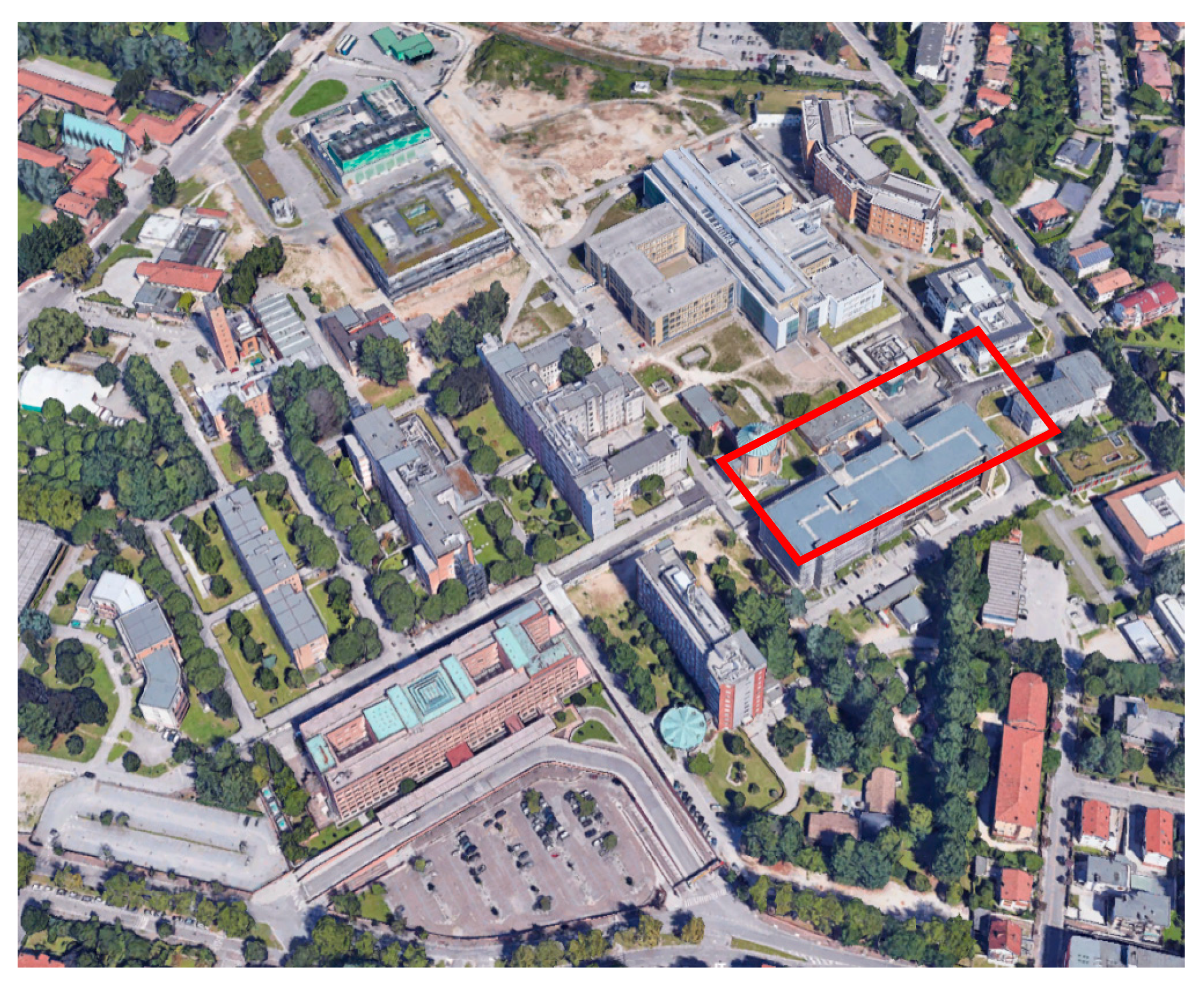
We applied the proposed model to a case study: pavilion No. 7 ‘Petracco’ of the ‘Santa Maria della Misericordia Hospital’ in Udine, Friuli—Venezia Giulia region, Italy (Figure 3). This application is a significant test, because pavilion No. 7 has been subjected to a final draft project to bring structural, fire safety, and technical plant adjustments up to regulation, due to the critical issues found in ordinary functionality.

This pavilion was built in 1980, and it consists of four above ground floors and a basement: a typical mono-block type with a load-bearing structure in reinforced concrete. The current use is mainly for patient hospitalization in Neonatal Pathology, Maxillofacial Surgery, and Orthopedics.

Table 15. General information concerning Santa Maria della Misericordia hospital in Udine.

Type of General Information	Notes
HIDP.1.1. Local Health Department	ASUIUD—Udine Integrated University Hospital
HIDP.1.2. Health facility	Santa Maria della Misericordia Hospital—Udine
HIDP.1.3. Typology of hospital	Pavilions
HIDP.1.4. Main period of construction	1924–1938; 1975–1985
HIDP.1.5. Buildings	No. 20 Pavilions
HIDP.1.6. Provided services	(1) Emergency, (2) Surgical Clinic, (3) Oncology, (4) Internal Medicine, (5) Anesthesia and Resuscitation, (6) Specialized Medicine, (7) Neurological and Neuroscience Clinic, (8) Diagnostic Imaging, (9) Cardiothoracic Surgery, (10) Transfusion Medicine, (11) Maternal and Child Department, (12) Laboratory, (13) Administration

and

Table 16. Scheduling subject features concerning each comparable historic intervention.

General Information on Subject Intervention
Intervention Features	Feature Characterization
Building subjected to intervention	Pavilion No. 7 ‘Petracco’
Main construction period	1968–1996
Complexity of prevailing provided service	Hospitalization
Structural typology	Concrete
Functional typology	Mono-block
Total building gross area [m2]	17,927.03
Total building gross volume [m3]	90,146.00
Overall glazing area [m2]	1441.40
Overall sediment area [m2]	3513.00
Overall vertical envelope area [m2]	7939.16

reveal the characteristics of the entire hospital and Pavilion No. 7 Petracco.

Table 17. Results for section QSS.1, concerning Pavilion No. 7.

QSS—Section QSS.1
Features	Selection	Values
QSS.1.1. Construction period	1968–1996	4
QSS.1.2. Latest intervention for structural adjustments/improvements	1987–1996	3
QSS.1.3. Latest energy refurbishment of opaque envelope	1977–1991	2
QSS.1.4. Latest energy refurbishment of transparent envelope	1977–1991	2
QSS.1.5. Installation period or latest requalification of HVAC systems and plants	2012–2015	4
QSS.1.6. Installation period or latest requalification of fire-extinguishing and fire-detection plants	2003–2012	3
QSS.1.7. Installation period or latest requalification of special and electric plants	1971–1990	2
QSS.1.8. Installation period or latest requalification of elevators and lift systems	<1997	1
QSS.1.9. Installation period or latest requalification of medical gas plants	2010–2017	3
QSS.1.10. Latest intervention for layout adjustment/architectural barrier removals	>1996	3
QSS.1.11. Latest intervention adjusting the infrastructures for contaminated waste disposal and waste storage areas	1997–2006	2

,

Table 18. Results for section QSS.2, concerning Pavilion No. 7.

QSS—Section QSS.2
Features	Selection	Values
QSS.2.1. Ground acceleration [m s−2]	≥0.125∙g	2
QSS.2.2. Heat degree, days [°C]	2200–2400	2
QSS.2.3. Dry periods, 5-mm-cumulative rainy days per year [mm]	60–75	2
QSS.2.4. Rainfall intensity [mm]	55–70	2
QSS.2.5. Activity risk profile	D2	5
QSS.2.6. Intended use of the space/area	Hospitalization	5
QSS 2.7. Structural typology	Concrete	2
QSS 2.8. Functional typology	Mono-block	1

and

Table 19. Results for section QSS.3, concerning Pavilion No. 7.

QSS—Section QSS.3
Features	Selection	Values
QSS.3.1. Balanced mechanical ventilation	None	1
QSS.3.2. Renewable energy systems for thermal energy production	None	1
QSS.3.3. Renewable energy systems for electricity production	None	1
QSS.3.4. Efficiency of thermal energy production system	<0.85	1
QSS.3.5. Efficiency of DHW production system	0.80–0.90	2
QSS.3.6. Dangerous materials in outdoor spaces/areas	Absent	1
QSS.3.7. Dangerous materials in indoor spaces/areas	Absent	1
QSS.3.8. Availability of relevant parking areas compared to gross cubic volume [m2 m-3]	>0.8	4
QSS.3.1. Balanced mechanical ventilation	None	1
QSS.3.2. Renewable energy systems for thermal energy production	None	1
QSS.3.3. Renewable energy systems for electricity production	None	1

report the results of the QSS subroutine applied to Pavilion No. 7, with the valorization of each feature necessary for the SI activation procedure.

Based on the SID and QTE subroutines,

Table 20. SIs activated by the QTE subroutine and related extensions.

SI Codes	Standard Interventions (SI)	Activation	Extension [%]
SS1	Global seismic reinforcement	YES	100
SS2	Seismic adjustment of HVAC systems and plants	no	-
SS3	Seismic adjustment of sanitary and fire-extinguishing plants	YES	100
SS4	Seismic adjustment of medical gas plants	no	-
SS5	Seismic adjustment of special and electric plants	YES	100
FS1	New fire compartmentalization/fire protection works	YES	90
FS2	Installation of fire-extinguishing hydrant plant/network	YES	20
FS3	Installation of fire-extinguishing sprinkler plant/network	YES	30
FS4	Sectioning of medical gases network	no	-
FS5	Installation of fire-detection plant	YES	100
FS6	Installation of fire escape elevator	YES	30
LS1	Improvement of storm water disposal system	no	-
LS2	Flooding protection works	no	-
LS3	Installation of flooding protection pumps	no	-
RF1	Works for architectural barrier removals	no	-
RF2	Functional adjustment of indoor and outdoor spaces	no	-
RF3	Installation/substitution of HVAC systems and plants	no	-
RF4	Modification of HVAC systems and plants	no	-
RF5	Installation/substitution of sanitary and fire-extinguishing plants	YES	20
RF6	Modification of thermal sanitary and fire-extinguishing plants	no	-
RF7	Installation/substitution of medical gas plants	no	-
RF8	Modification of medical gas plants	no	-
RF9	Installation/substitution of special and electric plants	YES	30
RF10	Modification of special and electric plants	no	-
RF11	Lift system adjustment	YES	80
EE1	Thermal insulation of opaque building envelope	YES	100
EE2	Enhancement of transparent building envelope	YES	100
EE3	New HVAC systems and plants for higher efficiency	YES	40
EE4	New DHW production systems for higher efficiency	no	-
EE5	New power production systems for higher efficiency	no	-
ES1	Improvement of infrastructures for contaminated waste disposal	no	-
ES2	Improvement of outdoor areas for waste storage	no	-
ES3	Removal of dangerous materials from outdoor spaces	no	-
ES4	Removal of dangerous materials from indoor spaces	no	-
ES5	Installation of renewable energy system for thermal energy production	no	-
ES6	Installation of renewable energy system for electricity production	YES	10
ES7	Installation of a storage and reuse system for rainwater	no	-
FA1	New parking areas	no

shows the activated SIs, associated with the relevant extensions and expressed in percentages: the ratio of the overall gross area of Pavilion No. 7. Thus, all of the activated SIs, characterized by each construction category’s intensity and the applied extensions, are available.

Table 21. Application of Case Based Reasoning (CBS) procedure to the case study: features optioneering.

Features		Construction Period (HIDP.2.2)	Service Complexity (HIDP.2.3)	Structural Typology (HIDP.2.4)	Functional Typology (HIDP.2.5)
Subject		1968–1996	First Aid/Operating Rooms/Intensive Care	Reinforced concrete	Mono-block
Comparable items	1	1968–1996	Hospitalization	Reinforced concrete	Tower
	2	1968–1996	Hospitalization	Reinforced concrete	Tower
	3	1968–1996	Hospitalization	Reinforced concrete	Tower
	4	1900–1938	Hospitalization	Masonry	Mono-block
	5	1939–1967	Ambulatory clinic	Reinforced concrete	Mono-block
	6	1939–1967	Ambulatory clinic	Reinforced concrete	Mono-block
	7	1939–1967	Laboratory	Reinforced concrete	Mono-block
	8	1968–1996	First Aid/Operating rooms/Intensive care	Reinforced concrete	Slab
	9	1968–1996	Laboratory	Reinforced concrete	Mono-block
	10	1939–1967	Laboratory	Reinforced concrete	Mono-block
	11	<1900	Ambulatory clinic	Masonry	Court
	12	<1900	Ambulatory clinic	Masonry	Court
	13	1968–1996	Ambulatory clinic	Reinforced concrete	Mono-block
	14	1968–1996	Laboratory	Reinforced concrete	Mono-block
	15	<1900	Ambulatory clinic	Masonry	Court
	16	1968–1996	Hospitalization	Reinforced concrete	Mono-block
	17	1968–1996	Hospitalization	Reinforced concrete	Mono-block
	18	1968–1996	Laboratory	Reinforced concrete	Backbone
	19	1968–1996	Hospitalization	Reinforced concrete	Mono-block
	20	1968–1996	Ambulatory clinic	Steel	Slab
	21	1968–1996	Hospitalization	Reinforced concrete	Tower

reports salient information for CBS procedure according to relevant data collected in HIDP, while

Table 22. Application of CBS procedure to the case study: individuation of similar interventions.

Coefficients		Jaccard	Sørensen	Average
Subject		(1.00)	(1.00)	(1.00)
Comparable items	1	0.50	0.67	0.58
	2	0.50	0.67	0.58
	3	0.50	0.67	0.58
	4	0.25	0.40	0.33
	5	0.50	0.67	0.58
	6	0.50	0.67	0.58
	7	0.50	0.67	0.58
	8	0.75	0.86	0.80
	9	0.75	0.86	0.80
	10	0.50	0.67	0.58
	11	-	-	-
	12	-	-	-
	13	0.75	0.86	0.80
	14	0.75	0.86	0.80
	15	-	-	-
	16	0.75	0.86	0.80
	17	0.75	0.86	0.80
	18	0.50	0.67	0.58
	19	0.75	0.86	0.80
	20	0.25	0.40	0.33
	21	0.50	0.67	0.58

reports the average score that was obtained in the application of qualitative similarity coefficients to individuate similar interventions. The similarity coefficients’ application excludes comparable items No. 4, 11, 12, and 15, as all the qualitative coefficients had a value below 0.5. Moreover, the Dice coefficient had values below 0.5 for all intervention comparable items.

Table 23. Calculated similarity coefficients and related estimated entitary costs.

Similarity Coefficients
		Steinhaus	Rudjichka	Kulczynski	Jaccard	Cosine	Dice
Selected comparable buildingsby CBS procedure	0–1	-	-	-	-	0.54	-
	0–2	-	-	-	-	0.54	-
	0–3	-	-	-	-	0.54	-
	0–5	-	-	-	-	0.72	-
	0–6	0.55	-	0.55	0.55	0.79	-
	0–7	-	-	-	-	0.52	-
	0–8	-	-	-	-	0.73	-
	0–9	0.53	-	0.53	-	0.79	-
	0–10	-	-	-	-	0.73	-
	0–13	-	-	-	0.54	0.74	-
	0–14	-	-	-	-	0.52	-
	0–16	0.56	-	0.68	-	0.58	-
	0–17	-	-	-	-	0.56	-
	0–18	-	-	-	-	0.5	-
	0–19	-	-	-	-	0.5	-
	0–21	0.68	0.51	0.7	0.65	0.88	-
Estimated entitary cost [€/entity]		836.36	1219.89	824.60	807.64	554.40	-
Average entitary cost [€/entity]		848.58

reveals entitary results according to Equation (19).

Finally, the cost of refurbishing the assessed building is calculated using an entitary cost (Equation (20)) through the non-zero value averages that were provided by the similarity coefficients.

$$C=\frac{{\sum }_{l=1}^{p}c{e}_l}{p}·A_0·I_0=848.58·17,927.04·51\%=7,728,222.31 €$$

(26)

6. Concluding Remarks

The proposed model shows the most probable cost of modernizing buildings. Furthermore, the reliability of the model’s result is strongly dependent on the number and quality of available intervention data. The greater the number of codified interventions, the greater the possibility of identifying similar/comparable interventions. It is also possible to subsequently raise the similarity coefficient’s threshold for the first and second phase selections. Generally, one must calibrate the threshold for both steps to have a sufficiently broad selection of similar comparable items.

The model’s validation is also important. Not much literature and price list data are available, as this study represents a cost valuation for modernizing special purpose facilities. Thus, we tested the model on a case for which refurbishment cost data is available. Starting from Jevons’ principle of indifference [6], we investigated the possibility of estimating modernizing costs for health facilities while using similarity coefficients that can weigh intervention costs, as comparable items based on their affinity with the examined building. We assessed coefficient use and their similarities in estimation, but their use is rather limited in this sense.

Overall, we presented a model that identifies modernization needs (technical performance evaluation) and estimates the costs. The first phase, using qualitative coefficients, selects the comparable items according to the building’s characteristics, while the second estimates the affinity between the compared and subject interventions using quantitative coefficients. The estimated similarity coefficient weighs the relevant intervention’s costs.

We believe that the model offers a good degree of reliability and a quick estimation based on a more detailed procedure when compared to simple parametric valuations. This approach can be used when the cost estimate aims to support the planning of a multi-annual investment budget for buildings refurbishment when they show structural, layout, and plants deficits with respect to current regulations. This tool can estimate the most probable cost of modernizing a special use building and partial interventions that do not concern overall modernization (substituting the performance evaluation). It can also help to estimate a financial budget for planning a series of actions and derive parametric costs for standard interventions.

The greater issue is the difficulties in finding a quick way to validate the results. In this case, the available refurbishment cost data for the examined building permitted the model’s validation. However, future studies should develop a validation that can serve for every application to increase the valuation results’ reliability Furthermore, it would be useful to test the model and verify its effectiveness on a greater number of buildings in order to use the results of the assessments to improve its applicability, reliability, and effectiveness.

References

- Morano, P.; Tajani, F.; di Liddo, F.; Anelli, D. A feasibility analysis of the refurbishment investments in the Italian residential market. Sustainability 2020, 12, 2503. [Google Scholar] [CrossRef] [Green Version]
- di Ludovico, M.; de Martino, G.; Prota, A.; Manfredi, G. Empirical damage and repair costs for the assessment of seismic loss scenarios. In XVIII ANIDIS Congress Seismic Engineering; Pisa University Press: Pisa, Italy, 2019. [Google Scholar]
- Dell’Anna, F.; Vergerio, G.; Corgnati, S.; Mondini, G. A new price list for retrofit intervention evaluation on some archetypical buildings. Valori Valutazioni 2019, 22, 3–17. [Google Scholar]
- Manganelli, B.; Mastroberti, M.; Vona, M. Evaluation of benefits for integrated seismic and energy retrofitting for the existing buildings. In New Metropolitan Perspectives ISHT 2018 Smart Innovation System Technologies; Springer: Cham, Switzerland, 2019; pp. 654–662. [Google Scholar] [CrossRef]
- Manganelli, B.; Vona, M.; de Paola, P. Evaluating the cost and benefits of earthquake protection of buildings. J. Eur. Real Estate Res. 2018, 11, 263–278. [Google Scholar] [CrossRef]
- Jevons, W.S. The Theory of Political Economy, 3rd ed.; Macmillan and Company: New York, NY, USA, 1888. [Google Scholar]
- Choi, S.-S.; Cha, S.-H.; Tappert, C.C. A survey of binary similarity and distance measures. J. Syst. Cybern. Inform. 2010, 8, 43–48. [Google Scholar]
- Trobisch, P.D.; Bauman, M.; Weise, K.; Stuby, F.; Hak, D.J. Histologic analysis of ruptured quadriceps tendons, Knee Surgery. Sports Traumatol. Arthrosc. 2010, 18, 85–88. [Google Scholar] [CrossRef] [PubMed]
- Hubalek, Z. Coefficients of association and similarity, based on binary (presence-absence) data: An evaluation. Biol. Rev. 1982, 57, 669–689. [Google Scholar] [CrossRef]
- Michael, E.L. Marine ecology and the coefficient of association: A plea in behalf of quantitative biology. J. Ecol. 1920, 8, 54–59. [Google Scholar] [CrossRef]
- Driver, H.E.; Kroeber, A.L. Quantitative Expression of Cultural Relationships; University of California Press: Berkeley, CA, USA, 1932. [Google Scholar]
- Sokal, R.R. A statistical method for evaluating systematic relationships. Univ. Kansas Sci. Bull. 1958, 38, 1409–1438. [Google Scholar]
- Smith, J.R.; Chang, S.-F. Automated binary texture feature sets for image retrieval. In Proceedings of the 1996 IEEE International Conference Acoustics Speech, Signal Processing Conference Proceedings, Atlanta, GA, USA, 7–10 May 1996; pp. 2239–2242. [Google Scholar]
- Hohn, M.E. Binary coefficients: A theoretical and empirical study. J. Int. Assoc. Math. Geol. 1976, 8, 137–150. [Google Scholar] [CrossRef]
- Willett, P.; Barnard, J.M.; Downs, G.M. Chemical similarity searching. J. Chem. Inf. Comput. Sci. 1998, 38, 983–996. [Google Scholar] [CrossRef] [Green Version]
- Forbes, S.A. On the Local Distribution of Certain Illinois Fishes: An Essay in Statistical Ecology; Illinois State Laboratory of Natural History: Champaign, IL, USA, 1907. [Google Scholar]
- Forbes, S.A. Method of determining and measuring the associative relations of species. Science 1925, 61, 518–524. [Google Scholar]
- Scardi, M. Data Analysis Techniques in Ecology. University of Rome, Department of Biology, 2009. Available online: http://www.michele.scardi.name/corsi/metodi.pdf (accessed on 24 July 2020).
- Rogers, D.J.; Tanimoto, T.T. A computer program for classifying plants. Science 1960, 132, 1115–1118. [Google Scholar] [CrossRef] [PubMed]
- Sneath, P.H.A.; Sokal, R.R. Numerical taxonomy. In The Principles and Practice of Numerical Classification; W.H. Freeman and Company: San Francisco, CA, USA, 1973. [Google Scholar]
- Jaccard, P. Étude comparative de la distribution florale dans une portion des Alpes et des Jura. Bull. La Société Vaud. Des. Sci. Nat. 1901, 37, 547–579. [Google Scholar]
- Sørensen, T.A. A method of establishing groups of equal amplitude in plant sociology based on similarity of species content and its application to analyses of the vegetation on Danish commons. Biol. Skr. Udg. Det K. Dan. Vidensk Selsk. 1948, 5, 1–34. [Google Scholar]
- Motyka, J. O Zadaniach i Metodach badań Geobotanicznych/Sur les buts et les Méthodes des Recherches Géobotaniques; Nakładem Uniwersytetu Marii Curie-Skłodowskiej: Lublin, Poland, 1947. [Google Scholar]
- Goodall, D.W. Sample Similarity and Species Correlation. In Ordination of Plant Communities; Whittaker, R.H., Ed.; Springer: Dordrecht, The Netherland, 1978; pp. 99–149. [Google Scholar] [CrossRef]
- Kulczyński, S. Die Pflanzenassoziationen der Pieninen; Bulletin de l’Académie polonaise des sciences. Série des sciences biologiques; Imprimerie de l’Université: Krakow, Poland, 1928. [Google Scholar]
- Tanimoto, T.T. IBM Internal Report 17th November 1957; IBM Company: Armonk, NY, USA, 1957. [Google Scholar]
- Dice, L.R. Measures of the amount of ecologic association between species. Ecology 1945, 26, 297–302. [Google Scholar] [CrossRef]
- Isakson, H.R. The nearest neighbors appraisal technique: An alternative to the adjustment grid methods. Real Estate Econ. 1986, 14, 274–286. [Google Scholar] [CrossRef]
- Mahalanobis, P.C. On the Generalized Distance in Statistics. Natl. Inst. Sci. India 1936, 2, 49–55. [Google Scholar]
- Isakson, H.R. Valuation analysis of commercial real estate using the nearest neighbors appraisal technique. Growth Chang. 1988, 19, 11–24. [Google Scholar] [CrossRef]
- Ciuna, M.; de Ruggiero, M.; Manganelli, B.; Salvo, F.; Simonotti, M. Automated Valuation Methods in Atypical Real Estate Markets Using the Mono-parametric Approach. In Computational Science Its Applications—ICCSA 2017; Gervasi, O., Murgante, B., Misra, S., Borruso, G., Torre, C.M., Rocha, A.M.A.C., Taniar, D., Apduhan, B.O., Stankova, E., Cuzzocrea, A., Eds.; Springer: Cham, Switzerland, 2017; pp. 200–209. [Google Scholar] [CrossRef]
- De Ruggiero, M.; Salvo, F. Misure di similarità negli adjustment grid methods. Aestimum 2011, 58, 47–58. [Google Scholar]
- Simonotti, M.; Salvo, F.; Ciuna, M.; de Ruggiero, M. Measurements of Rationality for a Scientific Approach to the Market-Oriented Methods. J. Real Estate Lit. 2016, 24, 403–427. [Google Scholar]
- Tajani, F.; Morano, P.; Salvo, F.; de Ruggiero, M. Property valuation: The market approach optimised by a weighted appraisal model. J. Prop. Investig. Financ. 2019. [Google Scholar] [CrossRef]
- Kulczycki, M.; Ligas, M. Qualitative similarity coefficients in real estate market analysis/Jakościowe współczynniki podobieństwa w analizie rynku nieruchomości. Geomat. Environ. Eng. 2014, 8, 33–41. [Google Scholar] [CrossRef]
- Zyga, J. Connection between similarity and estimation results of property values obtained by statistical methods. Real Estate Manag. Valuat. 2016, 24, 5–15. [Google Scholar] [CrossRef] [Green Version]
- Zyga, J. Data selection as the basis for better value modelling. Real Estate Manag. Valuat. 2019, 27, 25–34. [Google Scholar] [CrossRef] [Green Version]
- OCSE/Osservatorio Europeo Delle Politiche e Dei Sistemi Sanitari. Italia: Profilo Della Sanità 2019; OECD Publishing, Paris/European Observatory on Health Systems and Policies: Paris, France, 2019. [Google Scholar]
- Rosato, P.; Alberini, A.; Zanatta, V.; Breil, M. Redeveloping derelict and underused historic city areas: Evidence from a survey of real estate developers. J. Environ. Plan. Manag. 2010, 53, 257–281. [Google Scholar] [CrossRef] [Green Version]
- Flores-Colen, I.; de Brito, J.; Freitas, V. Discussion of criteria for prioritization of predictive maintenance of building façades: Survey of 30 experts. J. Perform. Constr. Facil. 2010, 24, 337–344. [Google Scholar] [CrossRef]
- Ali, A.; Hegazy, T. Multicriteria assessment and prioritization of hospital renewal needs. J. Perform. Constr. Facil. 2014, 28, 528–538. [Google Scholar] [CrossRef]
- Lavy, S.; Garcia, J.A.; Scinto, P.; Dixit, M.K. Key performance indicators for facility performance assessment: Simulation of core indicators. Constr. Manag. Econ. 2014, 32, 1183–1204. [Google Scholar] [CrossRef]
- Dejaco, M.C.; Cecconi, F.R.; Maltese, S. Key performance indicators for building condition assessment. J. Build. Eng. 2017, 9, 17–28. [Google Scholar] [CrossRef]
- Rechel, B.; Wright, S.; Edwards, N.; Dowdeswell, B.; McKee, M. Investing in Hospitals of the Future; WHO: Copenhagen, Denmark, 2009. [Google Scholar]
- Baraldi, G.; Capurso, L.; Costa, G.; Cuccurullo, F.; di Stanislao, F.; Gensini, G.; Guarini, R.; Mangia, R.; Mauri, M.; Montaguti, U.; et al. Principi guida tecnici, organizzativi e gestionali per la realizzazione e gestione di ospedali ad alta tecnologia e assistenza (Technical, organizational and managerial guiding principles for the construction and management of high technology hospitals). Monitor 2003, 6, 1–296. [Google Scholar]
- Head of Italian Government. Approval of Instructions for Hospital Construction; D.G.H. 20 July 1939; Head of Italian Government: Rome, Italy, 1939.
- Ministry of Public Works, Ministry of the Interior. Limits on Building Density, Height, Distance among Buildings and Maximum Ratios between Residential and Productive Settlements and Public Spaces or Spaces Reserved for Collective Activities, Public Greenery or Parking Areas; M.D. 2 April 1968 No. 1444; Ministry of Public Works, Ministry of the Interior: Rome, Italy, 1968.
- President of Italian Republic. Approval of the Act of Addressing and Coordination to Regions and Autonomous Provinces of Trento and Bolzano, in Relation to Minimum Structural, Technological and Organisational Requirements for the Exercise of Health Activities; D.R.P. 14 January 1997; President of Italian Republic: Rome, Italy, 1997.
- Ministry of Public Works. Approval of Technical Standards for Construction in Seismic Zones; M.D. 3 March 1975; Ministry of Public Works: Rome, Italy, 1975.
- Ministry of Public Works. Technical Standards for Seismic Buildings; M.D. 24 January 1986; Ministry of Public Works: Rome, Italy, 1986.
- Ministry of Public Works. Technical Standards for the Calculation, Execution and Testing of Structures in Normal and Pre-Compressed Concrete and of Metal Structures; M.D. 9 January 1996; Ministry of Public Works: Rome, Italy, 1996.
- Prime Minister’s Office. Early Features of General Criteria for Seismic Classification of the National Territory and Technical Regulations for Construction in Seismic zone; Ordinance 20 March 2003 No. 3274; Prime Minister’s Office: Rome, Italy, 2003.
- Ministry of Infrastructure. Approval of New Technical Standards for Construction; M.D. 14 January 2008; Ministry of Infrastructure: Rome, Italy, 2008.
- President of Italian Republic. Standards for Reducing Energy Consumption for Thermal Uses in Buildings; D.R.P. 30 April 1976 No. 373; President of Italian Republic: Rome, Italy, 1976.
- Italian Parliament. Rules for the Implementation of the National Energy Plan on the Rational Use of Energy, Energy Savings and the Development of Renewable Energy Sources; Law 9 January 1991 No. 10; Italian Parliament: Rome, Italy, 1991.
- Italian Parliament. Implementation of the 2002/91/EC Directive on Energy Performance in Construction; Lgs. D. 19 August 2005 No. 192.; Italian Parliament: Rome, Italy, 2005.
- Ministry of Economic Development, Ministry of Environment and Land and Sea Protection, Ministry of Infrastructure and Transportation. Application of Energy Performance Calculation Methodologies and Definition of Minimum Building Requirements; M.D. 26 June 2015; Ministry of Economic Development, Ministry of Environment and Land and Sea Protection, Ministry of Infrastructure and Transportation: Rome, Italy, 2015.
- Italian Parliament. Implementation of the 2009/28/EC Directive on Promoting the Use of Renewable Energy, with a Change and Subsequent Repeal of the 2001/77/EC and 2003/30/CE Directives; Lgs. D. 3 March 2011 No. 28; Italian Parliament: Rome, Italy, 2011.
- Italian Parliament. Provisional Nihil Obstat to Activities Subject to Fire Safety Control, Changes to Articles 2 and 3 of the Law 4 March 1982 No. 66, and Supplementary Rules for the Order of the Corpo Nazionale dei Vigili del Fuoco; Law 7 December 1984 No. 818; Italian Parliament: Rome, Italy, 1984.
- Ministry of the Interior. Approval of the Technical Fire Safety Regulation for the Design, Construction and Operation of Public and Private Health Facilities; M.D. 18 September 2002; Ministry of the Interior: Rome, Italy, 2002.
- Ministry of the Interior. Update of the Technical Fire Safety Regulation Attached to the Decree of the Minister of the Interior 18 September 2002; M.D. 19 March 2015; Ministry of the Interior: Rome, Italy, 2015.
- Ministry of the Interior. Code of Fire Safety; M.D. 3 August 2015; Ministry of the Interior: Rome, Italy, 2015.
- Italian Parliament. Provisions for the Production of Materials, Equipment, Machinery, Electrical and Electronic Installations and Systems; Law 1 March 1968 No. 186; Italian Parliament: Rome, Italy, 1968.
- Italian Parliament. Regulations for Plants Safety; Law 5 March 1990 No. 46; Italian Parliament: Rome, Italy, 1990.
- Ministry of Economic Development. Implementing Regulation of Article 11-Quaterdecies, Paragraph 13, Point b), of Law 2 December 2005, No. 248, about Reordering Provisions of Installation of Technical Systems in Buildings; M.D. 22 January 2008 No. 37; Ministry of Economic Development: Rome, Italy, 2008.
- Ministry of the Interior. Approval of the Technical Regulation about Fire Safety for Lift Compartments Located in Activities Subjected to Fire Control; M.D. 10 September 1996; Ministry of the Interior: Rome, Italy, 2005.
- President of Italian Republic. Regulation about Modication to D.R.P. 30 November 1999, No. 162, for the Application of 2014/33/UE Directive on Lifting Plants and Related Safety Components and Operation; D.R.P. 10 January 2017 No. 23; President of Italian Republic: Rome, Italy, 2017.
- Italian Parliament. Implementation of 93/42/CEE Directive about Medical Devices; Lgs. D. 24 February 1997 No. 46; Italian Parliament: Rome, Italy, 1997.
- Italian Parliament. Implementation of 2007/47/CE Directive Modifying Directives 90/385/CEE to Bring Member States Laws on Active Implantable Medical Devices Closer Together, 93/42/CE on Medical Devices and 98/8/CE on Biocides Market Entry; Lgs. D. 25 January 2010 No. 37; Italian Parliament: Rome, Italy, 2010.
- President of Italian Republic. Regulation for Implementation of art. 27 Law 30 March 1971 No. 118 in Favour of the Mutilated and Disabled Civilians, in Terms of Architectural Barriers and Public Transport; D.R.P. 27 April 1978 No. 384; President of Italian Republic: Rome, Italy, 1978.
- President of Italian Republic. Regulation for the Removal of Architectural Barriers in Buildings, Spaces and Public Services; D.R.P. 24 July 1996 No. 503; President of Italian Republic: Rome, Italy, 1996.
- Italian Parliament. Implementation of 89/618/Euratom, 90/641/Euratom, 96/29/Euratom e 2006/117/Euratom Directives in Ionizing Radiations; Lgs. D. 17 March 1995 No. 230; Italian Parliament: Rome, Italy, 1995.
- Italian Parliament. Implementation of 91/56/CEE Directive on Waste, 91/698/CEE Directive on Hazardous Waste and 94/62/CE Directive on Packaging and Packaging Waste; Lgs. D. 5 February 1997 No. 22; Italian Parliament: Rome, Italy, 1997.
- President of Italian Republic. Regulation on Sanitary Waste Management According to art. 24 Law 31 July 2002 No. 179; D.R.P. 15 July 2003 No. 254; President of Italian Republic: Rome, Italy, 2003.
- Italian Parliament. Environmental Standards; Lgs. D. 3 April 2006 No. 152; Italian Parliament: Rome, Italy, 2006.
- President of Italian Republic. Regulation for Design, Installation, Operation and Maintenance of the HVAC Systems in Buildings Aiming at the Reduction of Energy Consumption, in the Implementation of art. 4, Paragraph 4, of Law 9 January 1991 No. 10; D.R.P. 26 August 1993 No. 412; President of Italian Republic: Rome, Italy, 1993.
- European Commission, Commission Regulation (EC). No. 105/2007 of 1 February 2007 Amending the Annexes to Regulation (EC) No 1059/2003 of the European Parliament and of the Council on the Establishment of a Common Classification of Territorial Units for Statistics (NUTS), Official Journal of the European Union; European Union: Bruxelles, Belgique, 2007.
Figure 1.
Logical scheme of the Quick Requirement Assessment (QRA) procedure with its subroutines.
Figure 2.
Plotting of αj coefficient values (in ordinates) depending on the value (in abscissae).
Figure 3.
Location of Pavilion No. 7 in the Santa Maria della Misericordia hospital in Udine (satellite view by Google Maps®).