Investigations of HAWT Airfoil Shape Characteristics and 3D Rotational Augmentation Sensitivity Toward the Aerodynamic Performance Improvement

Abstract

This study investigates the impacts of different airfoil shapes on the 3D augmentation and power production of horizontal axis wind turbines (HAWTs). The aerodynamic effect from changing the leading and trailing edge of the airfoil is the emphasis of the research. Varied power produced from modifying sensitivity on 3D augmentations, caused by revamping airfoil shapes, are shown. The 3D correction law, considering the chord to radius ratio and the blades’ pitch angle in the rotation, is applied to the airfoil lift coefficients. The blade element method (BEM) embedded in the software Qblade with modified lift coefficients simulates the power productions of three wind turbines from these airfoils. The comparisons of the boundary layer characteristics, sectional forces, and inflow angle of the blade sections are calculated. The k-omega SST turbulence model in OpenFoam visualizes the stall and separation of the blades’ 2D section. The airfoils with a rounded leading edge show a reduced stall and separated flow region. The power production is 2.3 times higher for the airfoil constructed with a more rounded leading edge S809r and two times higher for the airfoil S809gx of the symmetric structure.

1. Introduction

Recently, the total installed capacity of wind energy over the world has been continuously increasing. Wind energy supplies the second largest capacity among different renewable energy sources in the most recent ten years [1]. As the demand and necessity for improving wind turbine performance increase, this study investigates the effective blade design for better performance of the wind turbine, mainly focused on the airfoil shape. Since the requirement of a rotating horizontal axis wind turbine rotor is different from the horizontal flying airplane wing, the need for the specific design of wind turbine airfoil has risen. The roughness sensitivity, higher gliding ratio, and structural stability on the root part with the tip part’s aerodynamic effectiveness are found to be some of several requirements of the airfoil in a wind turbine [2].

The National Renewable Energy Laboratory (NREL) designed several airfoils for both stall-regulated and pitch control wind turbines incorporated with the Solar Energy Research Institute (SERI) [3]. The team of Delft University of Technologyhas generated 15–40% thickness airfoils dedicated to the wind turbine [3,4]. The Risø national laboratory designed the thin-shaped airfoil for higher aerodynamic efficiency [5,6]. To make the airfoil suitable for the wind turbine application, the researchers have used various optimization strategies. The gradient-based optimization method searches for the solution by the convergence in the local solution of the function with the given derivatives. The example of airfoil design with the gradient method is in reference [7]. However, because of the flexibility of the design variable settings, stochastic methods such as genetic algorithms (GAs) have been used frequently for the airfoil design [8]. Chen used GA and artificial intelligence methods for increasing the lift to drag ratio of the airfoils [65]. The multi-objective GA is also applied to find the airfoil design for two objective functions, the maximum lift, and maximum gliding ratio by Chen [8]. Single and multi-objective genetic algorithms with the artificial neural network are used for novel airfoil design by Ribeiro with Computational Fluid Dynamics (CFD) coupling [9,10]. As the final optimum shape of the airfoil is from the vast numbers of candidate airfoil designs within the group called population, the GA optimization method is advantageous. The candidate designs in the population before the convergence can be saved and investigated for the other performance parameters. It is more useful for the current design research, as there is no need to devise an equation for the gradient-based optimization derivatives [7].

The researchers have designed the wind turbine airfoils from the 2D flow calculations before the concept of 3D rotational augmentation [11], mainly based on the blade element momentum (BEM) theory and the flow solver XFOIL [12,13]. However, it is essential to consider the 3D rotational flow situation in the airfoil design because the rotor’s lift coefficient shows a significant difference between 2D and 3D calculations. The rotation of the rotor is observed to increase the lift coefficient of the blade, especially in the inboard section, for example, by Himmelskamp [13], Ronsten [11], and Bruining [14].

In recent years, wind turbine size has increased to meet the increasing demand for clean energy supply. The enlarged wind turbine size can also be found in offshore applications with relevant research [15,16]. Like these, there is a need for thick airfoils with excellent structural stability [17]. However, the aerodynamic performance decreases as the blades take on thicker airfoils. A thinner airfoil leads the effective lifting of the blade while a thicker airfoil ensures structural strength. Therefore, the inverse relationship between the thickness and the aerodynamic performance, and the proportional relationship between the thickness and structural stability are the inevitable trade-off in the blade airfoil design. The structural stability and the excellent aerodynamic performance are two requirements to be satisfied in the airfoil of the large size rotors. As the rotor’s root is more exposed to the rotational flow, it is necessary to consider the airfoil’s design at the inboard part of the rotor with the 3D rotational augmentation [18].

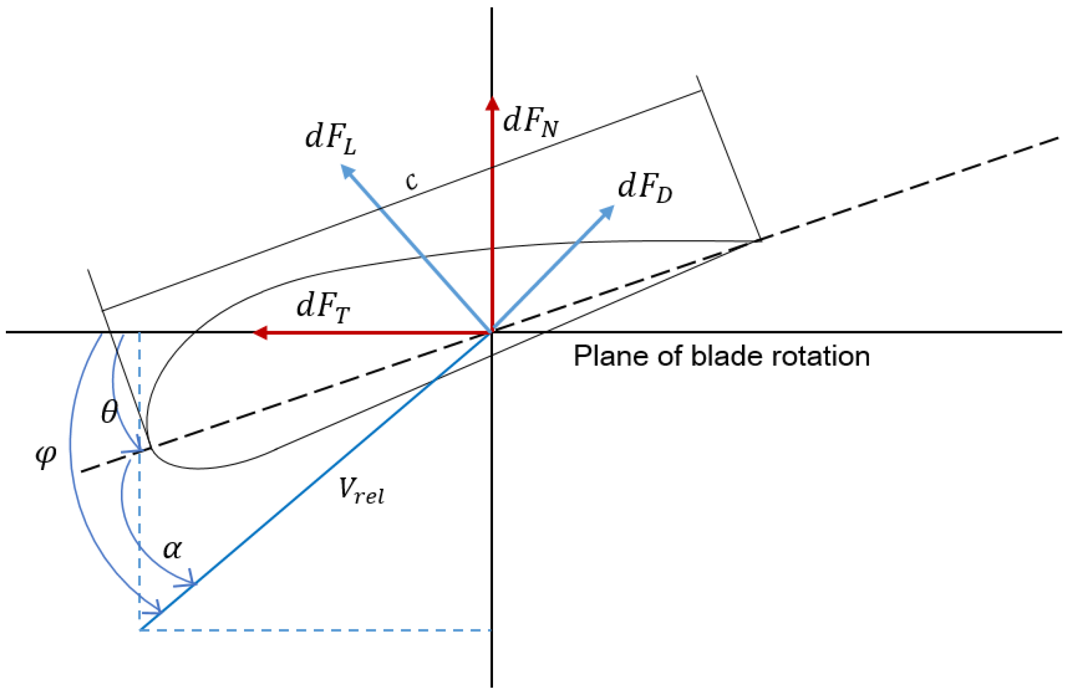
The angle of attack is the angle formed by the chord of the airfoil and the direction of the relative incoming wind [19]. As the complex rotational flow at the root section of the blade at the higher angle of attack with stall condition causes the secondary flow and the centrifugal force, a delay of flow separation happens at the part of the blade root. Moreover, the inertial forces from the rotation and the Coriolis force reduce the stall area at the blade sections in the rotational flow [20,21]. Therefore, the aerodynamics on the root part reduces the drag and increases the lift. Thus, the researchers have corrected the prediction models to supplement the absent physical description of the BEM theory as compensation.

Snell [22,23,24] derived a foundation for relating the 3D rotational augmentation with the ratio of the chord to the radius. This knowledge influenced several available empirical correction models in later years. An example of such correction was made, for instance, by Hansen and Chaviaropoulos. The semi-empirical correction law can be applied to correct the load coefficients. In general, the wind turbine has generated power in the 3D rotation 15–20% higher than in the 2D calculation [25]. Kim and Bangga [26] tried the airfoil shape comparison on different 3D rotational augmentation impacts.

The study of the relationship between an airfoil’s shape characteristics and its influence on the wind turbine performance became necessary to achieve an aerodynamically efficient and structurally stable airfoil in the blade inboard section with the dominant rotational flow. Sandia National Laboratories (SNL) inserted the blunt trailing edge airfoil in the inner region of the blade for the structural strength and aerodynamic efficiency at the same time [27]. However, Bangga found a significant unsteady flow and trailing edge separation at the thicker trailing edge [28].

The limit of the upper airfoil surface reduces the surface velocity around it. There is a connection between the position of the maximum thickness and the Gliding Ratio (GR). There is an impact from the nose radius from the leading edge of the airfoil on the blade performance. Moreover, the S-shaped tail of the airfoil is applied to improve the lift coefficient, although it has the possibility of turbulent separation [17]. The subtle difference of the airfoil shape properties such as curvature, thickness, camber line, nose radius, and tail sharpness influence the flow around the surfaces. The affected flow from the various shapes of the airfoil causes different velocity and pressure distribution over the curvature.

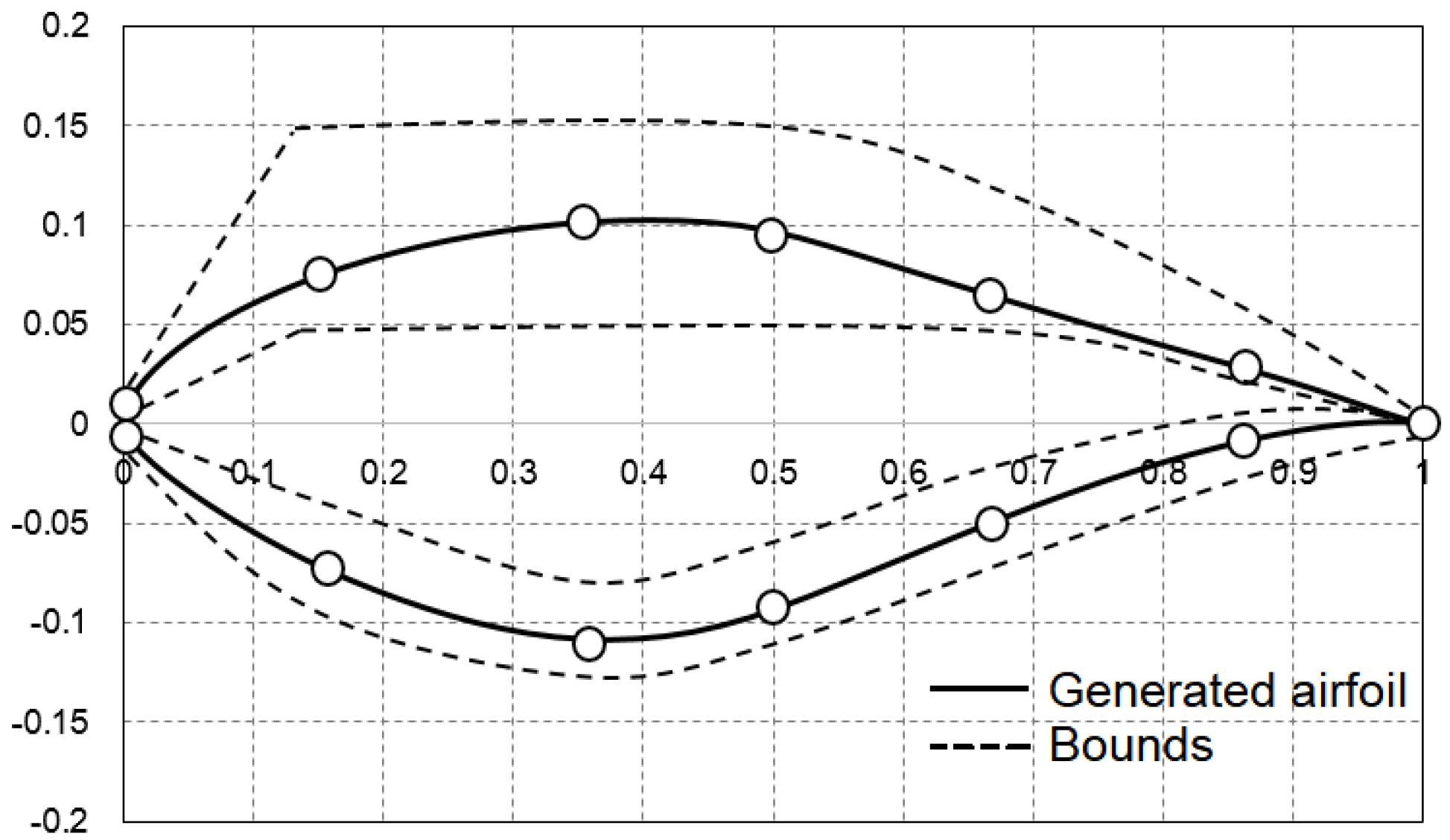
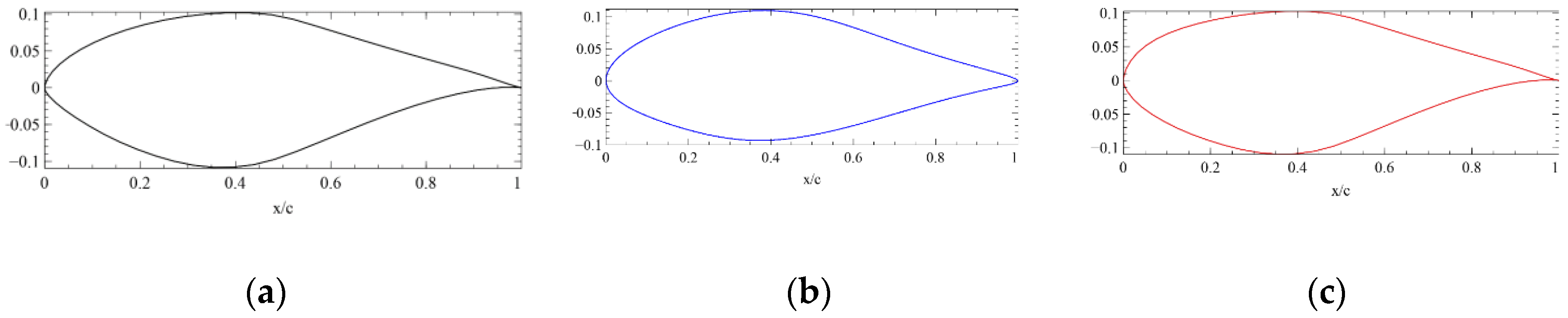
Because of the discrepancy of the 2D governing equation in the airfoil design with the rotational flow [12], it is necessary to research the airfoil’s sectional shape characteristics’ impact on the rotational flow. There is not much research in this field, but it has great potential to reveal the knowledge connected to the power improvement of the wind turbine. This study investigates the impacts of different airfoil shapes, which originated from the reference S809 of NREL Phase VI wind turbine [29]. Because of the mono airfoil type blade and sufficient experiment validation data, it is useful to check the direct impact of the sectional shape change of the blade on wind turbine power performance.

This research to find specific shape characteristics of the airfoils that influence the 3D rotational augmentation effect on the power of HAWT. Moreover, it also targets visualizing details on the 2D aerodynamics of the blade’s sectional shape with different airfoils. It also illustrates the stall differences caused by the airfoil shape change in detail. The 2D flow characteristics of three airfoils, its 3D-corrected lift data, and its blade’s power performance describe the relationship between airfoil shapes and aerodynamic performance in 3D rotational flow. Section 2 introduces the method and material used in the study, Section 3 presents all the results, and Section 4 explains the physics and reasons behind the results based on the given wind turbine performance theory and physics.

2. Materials and Methods

2.1. Airfoil and Blade Design

2.1.1. Airfoil Design

The B-spline method mathematically describes the airfoil [30]. The flexibility on the degree of accuracy makes B-spline shape almost any kind of desired airfoil. As the B-splines can precisely shape the reference airfoil to generate variously optimized airfoil shapes delicately, the B-spline airfoil parametrization is adopted in this section [7]. The spline functions curves consist of a piecewise polynomial approximation to make the additional smoothness possible. The recursive definition with the starting point $B_i^0\left(x\right)$ describes the B-spline, Equation (1).

$$B_i^k\left(x\right)=\left(\frac{x-t_i}{t_{i+k}-t_i}\right)B_i^{k-1}\left(x\right)+\left(\frac{t_{i+k+1}-x}{t_{i+k+1}-t_{i+1}}\right)B_{i+1}^{k-1}\left(x\right) \left(k\ge 1\right)$$

(1)

The set of knots is {$t_i$}, k = 1, 2, …, and i = 0, $\pm 1,$$\pm 2$. This study uses the B-spline airfoil with 13 control points and k order seven according to its proven usefulness in reference [31], see Figure 1.

As the optimal shape of the airfoil can be found in the vast numbers of candidate airfoil designs within the group called population, a genetic algorithm (GA) optimization method is used. It is more useful for the current design research, as there is no need to devise an equation for the gradient-based optimization derivatives [7]. The candidate designs in the population before the convergence can be saved and investigated for the other performance parameters. The airfoil S809gx is generated by the genetic algorithm (GA) optimization method with the objective function of a higher gliding ratio (GR) and transition point (Xtr) at Re = ${10}^6$, and alpha = 7°. The population size 5, generation number 100, and mutation adapt feasible options are used in the GA [32]. The $y$ points of control points in B-spline are under the given bounds, and the GA runs to find the airfoil shaped with different y points. Therefore, the constraints of this current are the range of y points of the airfoil in B-spline. Among the different airfoil shapes generated within the upper and lower bounds of y control points, the algorithms converge to the final airfoil with the highest objective function value. The objective function targets the GA to find the airfoil with the highest GR and transition point at the top and bottom surfaces. The objective function is the following, Equation (2). The algorithm converges at the minimum point, therefore, the objective function is set to be a minus value. The terms $T{X}_{tr}$and $B{X}_{tr}$ stand for the transition point at the top and bottom of the airfoil surface. The $(\frac{C_l}{C_d}$) in Equation (2) calculates the GR of the airfoil. The GA codes with B-spline upper and lower bounds and optimization conditions are found in reference [33].

$$f=\{-\left(\left(\frac{C_l}{C_d}\right)+T{X}_{tr}+B{X}_{tr}\right)\}$$

(2)

The reference airfoil is the airfoil S809 of NREL Phase VI [24]. Based on the increased GR values of the airfoil S809gx and the wind turbine’s power performance, the airfoil S809r is made. Inspired by the rounded nose shape of the airfoil S809gx, the airfoil S809r has a more rounded leading edge compared to the reference, see Figure 2.

The pressure, lift, drag coefficients, and other inviscid and viscid flow parameters are calculated by software XFOIL [12]. This software uses the integral boundary layer approach. It also includes the linear-vorticity stream function in the inviscid flow solver and viscous displacement effects. With the vortex sheet strength $\gamma$, source sheet strength $\sigma$, vector angle $\theta$, the variable $s$ along with the vortex, the vector magnitude $r$between the points $s$, and flow field (x, y), the stream function is the following, Equation (3).

$$\psi \left(x, y\right)= u_{\infty }y-v_{\infty }x+\frac{1}{2\pi }{\displaystyle \int }\gamma \left(x\right)lnr\left(s;x,y\right)ds+\frac{1}{2\pi }{\displaystyle \int }\sigma \left(s\right)\theta \left(s;x,y\right)ds$$

(3)

The explicit Kutta condition closes the equation, and the airfoil surfaces and the wake trajectory discretization are made with the flat panels with nodes N. The viscous flow is calculated by the two-equation lagged dissipation integral boundary layer formulation. It also uses the $e^n$ transition criterion. The details are found in reference [34].

The boundary layer of airfoil calculation from XFOIL is based on the boundary layer theory [16]. The flow around the thin flat or airfoil has two parts: inviscid flow and viscid flow. The viscid flow is the flow that receives the dominant viscous effect. The boundary layer is the region close to the surface wall where the viscosity has to be considered. The fluid inside this region is ordinarily laminar at first, and then the fluid turns to the turbulence from the inertial forces and the impacts from the outer flow. The surface shape of the airfoil and pressure distribution over the surface causes the point of this transition. The significant increases in the thickness and wall shear stress are found at the turbulent flow [35].

When the pressure distribution along the surface is too strong for fluid particles to overcome, the flow reversion occurs. The fluid particles move in the opposite direction to the mainstream. The reversed flow from the intense pressure distribution at the inviscid flow is called separation. The separated flow makes the stall region, where the rotating velocity of the flow is formed. The separated flow causes a significant increase in fluid momentum and drag. When the separation occurs at the laminar part of the boundary layer and attaches to the surface of the geometry, it becomes the laminar separation bubble. The flow over the airfoil without separation makes the lift producing flow around the blade. However, when the separation occurs, the flow is disturbed to make the lift of the blade. It is from the increased drag from separation and stall. It is necessary to consider the block of the separation of the flow at the airfoil for the blade design [36,37].

2.1.2. Blade Design

In this section, the description of the general blade design employed in the studies is presented, see Figure 3. The blade is based on the reference [24] blade specification. The airfoil type is the only variation. The radial position is $\mathrm{r}$, Chord length is $\mathrm{c}$, and twist angle is $\mathsf{\phi }$ in

Table 1. Specification of the blade characteristics employed in the studies.

r	c	φ	Airfoil
0.508	0.218	0	Circular
0.66	0.218	0	Circular
0.883	0.183	0	Circular
1.008	0.349	0	Circular
1.067	0.441	0	Circular
1.133	0.544	0	Circular
1.257	0.737	20.04	S809/gx/r
1.343	0.728	18.07	S809/gx/r
1.51	0.711	14.29	S809/gx/r
1.648	0.697	11.91	S809/gx/r
1.952	0.666	7.98	S809/gx/r
2.257	0.636	5.31	S809/gx/r
2.343	0.627	4.71	S809/gx/r
2.562	0.605	3.42	S809/gx/r
2.867	0.574	2.08	S809/gx/r
3.172	0.543	1.15	S809/gx/r
3.185	0.542	1.115	S809/gx/r
3.476	0.512	0.494	S809/gx/r
3.781	0.482	−0.015	S809/gx/r
4.023	0.457	−0.381	S809/gx/r
4.086	0.451	−0.475	S809/gx/r
4.391	0.42	−0.92	S809/gx/r
4.696	0.389	−1.352	S809/gx/r
4.78	0.381	−1.469	S809/gx/r
5	0.358	−1.775	S809/gx/r

.

2.2. BEM Method and 3D Correction Law

2.2.1. Blade Element Momentum Theory

The classical wind turbine performance calculation is from the theory of Glauert in the 1930s [38]. The basis of the derivation is from the linear one-dimensional momentum theory, according to the Froude–Rankine stream tube theory [6]. This theory assumes the steady, inviscid, incompressible, and axisymmetric flow around the rotor in the control volume [39]. This theory comprises the conversation of mass, energy, axial, and angular momentum over the control volume. The air control volume surrounds the model wind turbine, which has the cross-sections. The wind turbine is assumed the “actuator disc”. The net force on the control volume is equal to the net force of the force on the wind turbine [38].

When the wind blows through the turbine rotor, a pressure drop occurs in one-dimensional momentum theory. This pressure drop is energy loss. The missing energy in the axial flow becomes the rotational momentum of the stream tube, which is the reaction to the rotational torque. In this process, the rotation of the annular stream is generated [39], see Figure 4 and Figure 5

Bernoulli’s equation can explain the pressure and the velocity changes over the rotor and control volumes. $p_1$is the ambient pressure, $p_2$ is the pressure at the upstream of the rotor disc, and $p_3$ is the pressure at the downstream from the rotor disc. $U_1$is the inflow velocity, $U_2$ is the velocity at the rotor disc, and $U_3$ is the velocity at the far downstream, see Equations (4) and (5).

$$p_1+\frac{1}{2}\rho U_1{}^2= p_2+\frac{1}{2}\rho U_2{}^2$$

(4)

$$p_3+\frac{1}{2}\rho U_2{}^2= p_1+\frac{1}{2}\rho U_3{}^2$$

(5)

Each stage of the rotating annular stream tube from stages 1 to 4 are in Figure 4. After wind passes through steps 2 to 3, the wind rotates to make the rotational flow, called a wake. When the angular velocity of the rotating flow is $\omega$ with the blade angular velocity $\mathsf{\Omega }$, the conservation of momentum makes the torque calculation available. Based on the rotor radial element concept in Figure 5, the elemental torque can be found with the rotating annular element of fluid at radius $r$ in Equation (6).

$$dQ=d\dot{m}\left(\omega r\right)r=\rho U_{2}2\pi rdr\left(\omega r\right)r$$

(6)

The distinct radial elements of the rotor in BEM theory involve two assumptions: (1) no aerodynamic interactions within the 2D airfoil elements in each section and (2) the forces on each element are only generated from the lift and drag properties of airfoil shape and its relative inflow [41]. The airfoil and the relevant velocity angles in each section are in Figure 6.

Based on the rotor section concept, the parameters calculated at the sections of each airfoil are stacked to produce final torque, thrust, power, etc. The incoming velocity is $v$, angle of attack is $\alpha$, and incoming flow angle is $\psi$. The sectional tangential force and normal force are $d{F}_T$ and $d{F}_N$. The sectional lift and drag force are $d{F}_L$ and $d{F}_D$. With the lift coefficient $C_L$, drag coefficient $C_D$, and air density $\rho$, the following equations give the lift; drag forces; and tangential, normal forces. The section torque $dT$ and power $dP$ are also calculated, see Equations (7)–(12).

$$d{F}_L=C_L \frac{1}{2}\rho v^{2}cdr$$

(7)

$$d{F}_D=C_D \frac{1}{2}\rho v^{2}cdr$$

(8)

$$d{F}_T= \frac{1}{2}\rho v^{2}cdr\left(C_L\sin \left(\phi \right)-C_D\cos \left(\phi \right)\right)$$

(9)

$$d{F}_N= \frac{1}{2}\rho v^{2}cdr\left(C_L\cos \left(\phi \right)+C_D\sin \left(\phi \right)\right)$$

(10)

$$dT = Brd{F}_T$$

(11)

$$dP=Bd{F}_{T}r\omega$$

(12)

2.2.2. 3D Correction

The lift coefficients calculated by 2D airfoil flow solver XFOIL [12] at each section of the blades are extracted and corrected by the following 3D correction law from Chaviaropouls and Hansen [18]. This 3D correction proved to have highly increased predictability in a stall-regulated wind turbine. Compared to the other 3D correction models by Snel and Lindenburg [40], this method shows higher accuracy on NREL S809 airfoil lift coefficient corrections. The correction law formulation is based on the observation of the differences between the 2D and the quasi-3D curve and the semi-empirical correction law from Snel [23]. The 3D correction law to include rotational effect and the twist angle impact are derived as below Equation (13).

$$C_{l,3D}=C_{l,2D}+a{\left(\frac{c}{r}\right)}^{h}co{s}^n\left(twist\right)\mathsf{\Delta }{C}_l$$

(13)

where the $a$ = 2.2, $h$ = 1, $n$ = 4. The chord and radius ratio ($\frac{c}{r}$) and twist angle $\left(twist\right)$of each section are modulated for each blade section. The generated Cl values are extrapolated by Viterna [41] in Qblade [42]. As it offers the easily accessible estimation of the post-stall Cl and Cd values from the geometry, the Viterna method was chosen in this study [30]. Based on the data, the extrapolation of the stall angle of attack to angle 90° is calculated by the following Equations (14)–(19).

$$C_L=A_{1}sin2\alpha +A_2\frac{co{s}^2\alpha }{sin\alpha }$$

(14)

$$C_D=B_{1}si{n}^2\alpha +B_{2}cos\alpha$$

(15)

$$A_1=\frac{C_{Dmax}}{2}$$

(16)

$$B_1=C_{Dmax}$$

(17)

$$A_2=\left(C_{Lstall}-C_{Dmax}sin{\alpha }_{stall}cos{\alpha }_{stall}\right)\frac{sin{\alpha }_{stall}}{co{s}^2{\alpha }_{stall}}$$

(18)

$$B_2=\frac{C_{Lstall}-C_{Dmax}si{n}^2{\alpha }_{stall}}{cos{\alpha }_{stall}}$$

(19)

The reflection of the calculation is made for the airfoil data at the angle of attack larger than $90$°. The validity of the Viterna extrapolation method is in reference [41].

2.3. CFD Simulation

2.3.1. Airfoil

The aim of the simulations in this section is to visualize the different stall characteristics. Before the mesh generation steps, this section compares the subtle airfoil shape differences. Compared to the reference airfoil S809, the airfoil S809gx has a more symmetric and rounded nose, and the airfoil S809r has a more rounded shape in the leading edge, see Figure 7. The thickness of the three airfoils is similar to 20–21%, see

Table 2. Airfoil thickness and camber.

Airfoil	Thickness (%)	at (%)	Camber (%)	at (%)
S809	20.99	38.30	0.99	82.30
S809gx	20.30	38.70	0.87	43.60
S809r	21.18	38.20	0.99	82.30

.

2.3.2. Mesh Generation

The computational grid was generated using mesh generated by the built-in mesh generator of the SimFlow [43]. The surface cell thickness is 2 × ${10}^{-4}$ [m] and minimum surface cell length is 2 × ${10}^{-3}$. The cell number and minimum y+ at upper and lower surfaces in Re = $1.5 \times {10}^6$ are shown in

Table 3. Airfoil mesh information.

Airfoil	Cell Number	Upper y+	Lower y+
S809	60257	0.151	0.155
S809gx	60455	0.155	0.242
S809r	60653	0.155	0.242

.

The inlet, outlet, top, bottom, front, back, etc. were set in the geometry before it was calculated in the CFD solver. Figure 8 presents the close-up view near to the wall of the airfoil. Figure 9 shows the size of the whole mesh and the geometry setting of the airfoil.

2.3.3. k − ω SST Turbulence Model

At the moderate angle of attack (alpha), Spalart–Allmaras and models are used to predict the airfoils’ flow characteristics. However, at the angle of attack, regimes that generate the stall flow over the airfoil show different discrepancies and divergence [44,45]. Therefore, the agreement between the simulation results and experimental data at the chosen angle of attack in CFD should be checked. The $k-\omega$ SST turbulence model consumes lower computational costs than direct numerical simulation (DNS) and (large eddy simulation (LES). Moreover, it also shows fairly good agreement on the values in the 20-degree stall. Although the variations of the CFD results exist from different models at the stall angle of attack, the $k-\omega$SST model at the higher angle of attack is more sensitive at stall angle of attack than the $k-\epsilon$ model [46] and the validity check by this study, see Figure 10.

Mentor upgraded the $k-\omega$ model by Wilcox to be $k-\omega$SST model. This two-equation eddy-viscosity model uses the $k-\omega$ equations in the viscous dominant region, the boundary layer of the fluid. The $k-\epsilon$ model is applied in the non-viscous dominant region, free stream. This model improves the prediction accuracy of the separation and adverse pressure gradient predictions. The $k$ stands for the turbulent kinetic energy when the $\omega$ is for the eddy dissipation rate. The model is outlined in Equations (20)–(21) with the detailed coefficients from references [46,47].

$$\frac{\partial k}{\partial t}+U_j\frac{\partial k}{\partial x_j}=P_k-\beta \ast k\omega +\frac{\partial }{\partial x_j}\left[\left(\nu +{\sigma }_k{\nu }_T\right)\frac{\partial k}{\partial x_j}\right]$$

(20)

$$\frac{\partial \omega }{\partial t}+U_j\frac{\partial \omega }{\partial x_j}=\alpha S^2-\beta {\omega }^2+\frac{\partial }{\partial x_j}\left[\left(\nu +{\sigma }_{\omega }{\nu }_T\right)\frac{\partial \omega }{\partial x_j}\right]+2\left(1-F_1\right) {\sigma }_{\omega 2}\frac{1}{\omega }\frac{\partial k}{\partial x_i}\frac{\partial \omega }{\partial x_i}$$

(21)

2.3.4. Open Foam

The CFD simulation software OpenFOAM is used to compute the airflow around the airfoils because of its high accessibility without the license cost [48]. It is an open software employing a C++ library. As the flow simulation around the airfoil is under the incompressible flows with turbulence modeling, the solver SimpleFoam is adopted. This study takes the steady flow conditions. The computation assumes a fully turbulent boundary layer. The Semi-Implicit Method for Pressure Linked Equations (SIMPLE) algorithm solves the continuity and momentum equation. Each equation receives the solution from the previous steps. The objectives of the iteration steps are to produce the pressure field, free velocity field, and solved turbulence equation [49,50].

2.4. Method Validation

Validation Data

This section aims to show the agreement between the calculated results in Section 3 with the experiment data [24,28,36,51,52,53]. The simulation adopts the boundary conditions as the conditions from the reference experiments. The lift, drag coefficient, and transition point calculations are based on the Re =${10}^6$ in Figure 11 and Figure 12. The lift coefficients corrected by 3D correction law are representatively at radius 2.562 m (46%) of the blade with the 3D rotating experimental result [51,53] in Figure 13. The power results calculated by BEM with corrected Cl from 3D correction law are compared to the power measurement from the experiment [28] depicted in Figure 14.

The pressure coefficient (Cp) values show good agreement for the CFD results, especially for predicting the pressure recovery near the trailing edge compared to the XFOIL results, as shown in Figure 10a–d with experimental data [3]. The pressure prediction at the leading edge is far more accurate by OpenFoam than XFOIL at alpha = 20°. The airfoil chord position (x/c) is the x-axis, and the pressure coefficient (Cp) is the y-axis in Figure 10. Although the XFOIL calculation shows its limit on the lift and drag coefficient value prediction, the XFOIL results corrected by the 3D correction show the improved prediction. This is because 3D correction incorporates the rotational augmentation effect, which changes the parameters at the stall alpha, as shown in Figure 13 and Figure 14. However, the overprediction of the 3D-corrected BEM at the higher velocity decreases the prediction accuracy of the power production in Figure 14. The following sections analyze the results under the velocity of 15 m/s, where the prediction accuracy is relatively high.

3. Results

3.1. Aerodynamics

The lift, drag, and pressure coefficients for two different Re number situations are calculated, see Figure 15, Figure 16, Figure 17 and Figure 18. First, Re = $0.55 \times {10}^6$ with free stream velocity 8.5 m/s and Re = ${10}^6$ with the free-stream velocity 15 m/s. The modified leading-edge radius airfoil S809r shows the highest lift coefficients at both Re conditions. The airfoil s809r shows the larger lift coefficients at the higher alpha regime, which show its better tolerance at the stall effect. Moreover, the reference airfoil S809 shows the highest drag at both Re regimes.

It shows that the rounder nose airfoil S809r has increased GR values at the higher alpha, although its maximum is decreased. The airfoil S809gx still has the higher GR ratio at the stall alpha regime, but its less sharp trailing edge shape leads to its lower GR at the stall area than the S809r. The most substantial pressure difference at the leading edge of the reference airfoil leads to its more drastic adverse pressure gradients over the airfoil surface than the airfoil S809gx and S809r. The rounder leading edge with sharp trailing edge airfoil shows the milder pressure difference, as shown in the pressure coefficient plot in Figure 18, which indicates the less adverse pressure gradient having delayed separation.

3.2. CFD Results

The OpenFoam pressure distribution results compared to the experimental data at alpha 12.2° and 20° show higher predictability in Figure 10. As the lift and drag coefficients are from the pressure distribution around the airfoil, the experimental and CFD calculated Cl and Cd values also show good agreement on both alpha degrees in

Table 4. Cl, Cd of S809 at Re = 1.5 × ${10}^6$ from experiment [36] and CFD.

Method	Cl	Cd	Alpha
Experiment	1.00	0.04	12.2°
OpenFoam	1.06	0.05	12.2°
Experiment	0.850	0.202	20°
OpenFoam	0.852	0.222	20°

and Figure 19. The rounded nose airfoil S809r has the highest lift coefficient, whereas the airfoil with the highest symmetricity shows the smallest drag coefficient. The different stall characteristics around the airfoils also explain the drag difference caused by different airfoil shapes.

The stall simulation visualizations for the three airfoils—S809, S809r, and S809gx—are made at alpha 20. The lift and drag coefficients comparisons are shown in

Table 5. Cl, Cd of S809 at Re = 1.5 × ${10}^6$ for each airfoil by OpenFoam.

Airfoil.	Cl	Cd	Alpha
S809	0.852	0.222	20°
S809gx	1.133	0.117	20°
S809r	1.189	0.151	20°

and Figure 20. The pressure coefficient and velocity magnitude contours around the airfoil at Re = $1.5 \times {10}^6$ and alpha 20° are presented in Figure 21 and Figure 22, respectively. The sharp leading edge of the reference airfoil causes the most significant pressure gap at the nose part of the airfoil, which leads to the drastic adverse pressure gradient compared to the airfoils with the rounder nose leading edge. The pressure increase over the upper surface is the most mildly progressed in the S809r with the rounder leading edge. The flow under the less adverse pressure gradient field over the upper airfoil surface causes the less trailing edge vortex. As the trailing edge is less sharp at the airfoil S809gx than the airfoil S809r, the airfoil S809gx has less vortex at the trailing edge which reveals that the fluid progression influences the flow at the trailing edge from the upper surface curvature to the trailing edge shape. However, the airfoil S809r, which has the sharp S-tail trailing edge and the rounded nose, has the most delayed flow separation. It reveals that the roundness of the airfoil nose more influences the flow separation than the trailing edge sharpness and symmetry of the airfoil. It is beneficial to use the unsteady method, such as Unsteady Reynolds Averaged Navier Stokes (URANS), for the massively separated flow occurring on the reference airfoil. Some errors might occur with the simplification of steady-state conditions, but the reference airfoil is already at massively separated flow at the large angle of attack region, while the other two optimized airfoils are not. This conclusion should be general, independent of the steady Reynolds Averaged Navier Stokes (RANS) or the unsteady URANS simulations.

3.3. Transition Point (Xtr) in the Boundary Layer

The transition points where the boundary layer turns turbulent from the laminar at different angles of attack are described in Figure 23a. The airfoil S809gx which was designed to have the higher laminar boundary layer over all alpha ranges mostly has the highest laminar region on the upper and lower surfaces of the airfoil, especially at alpha > 10°. However, the rounder leading edge airfoil S809r has the broader laminar boundary layer region at a higher angle of attack. The S809r has a more extensive laminar boundary layer at the higher angle of attack on the upper surface. It is from the rounded nose part of the geometry. In the upper surface of airfoils, the rounded nose at S809r and S809gx causes less change in flow velocity stream and following pressure distribution over the airfoil surface. The smoother flow stream from the less adverse pressure gradient allows the flow particles inside the boundary layer to remain in laminar flow in contrast to the airfoil with a less rounded nose. The leading-edge radius influences the fluid particles inside the boundary layer at the bottom surface less. The symmetricity and the smoothness of the curve affect the transition of the particles from the laminar to turbulence. Although the less symmetric and S-shaped curve of the airfoil S809r and S809 have earlier transition points than the airfoil S809gx in the lower surface, the rounded nose airfoil S809r has the more extensive laminar boundary layer than the less rounded nose at the higher angle of attack.

3.4. Performance Analysis

3.4.1. 360° Extrapolation and Power Production

The lift coefficients corrected with the 3D correction law at each airfoil are extrapolated with the Viterna method, as shown in Figure 24a. This extrapolated polar data is located in the inboard region at r/R = 0.23. In this section, the chord to radius ratio is large, causing the stall to be delayed significantly for all three airfoils. The power distributions from the three wind turbines with the blades of the airfoil S809, S809gx, and S809r are calculated by the BEM method. The wind turbine with the airfoil S809gx shows about two times higher power and the turbine with the airfoil S809r produces c.a. 2.3 times higher power than the reference wind turbine, as shown in Figure 24b. The wind turbine with the airfoil S809r shows the most considerable increase in the higher velocity.

3.4.2. Cl and Tangential Force Over Blade

The lift coefficients and tangential forces over the blade position at the velocity 10 m/s (Tip Speed Ratio = 4.0) are depicted in Figure 25a,b. This condition marks the point where the generated power by the three investigated wind turbines is significantly different. The lift coefficient and the tangential force of the root section of the blade shows the airfoil S809r has the highest increase. As the 3D rotational augmentation is the most evident on the root section of the blade, the airfoil S809r receives the most enhancement from the 3D rotational effect. The airfoil S809gx also has a more considerable improvement than the reference. Although it has smaller Cl and tangential force in the tip, the higher values at the root imply that its shape benefits from the 3D rotation. The inflow angle of attack (Phi, $\varnothing$) over the blade position is also shown in Figure 25c. One can see that the angle of attack seen by the blade section composed by the baseline airfoil is larger than the other two modified airfoils for most radial sections. These findings indicate that the whole blade section of the reference airfoil already undergoes stall compared to the other two airfoils, causing performance reduction. This characteristic is also present in the nonlinearity occurring in the lift and tangential force distributions.

At 1.28 m of the blade in the root part, the lift coefficient and the tangential force are the highest. The inflow angle, lift, and drag coefficients of three airfoil blades at pos=1.28 are written in

Table 6. Inflow angle, lift, drag, tangential, and normal force coefficients at pos = 1.28 m.

Airfoil	$\varnothing [°]$	${\mathit{C}}_{\mathit{l}}$	${\mathit{C}}_{\mathit{d}}$	${\mathit{C}}_{\mathit{l}}\mathbf{sin}(\varnothing )-{\mathit{C}}_{\mathit{d}}\mathbf{cos}\left(\varnothing \right)$	${\mathit{C}}_{\mathit{l}}\mathbf{cos}(\varnothing )+{\mathit{C}}_{\mathit{d}}\mathbf{sin}\left(\varnothing \right)$
S809r	35.8	2.10	0.06	1.180	1.738
S809gx	34.8	2.16	0.09	1.159	1.825
S809	39.3	1.32	0.33	0.581	1.230

. Based on the tangential and normal force coefficient equations (columns 5 and 6, respectively), the corresponding force coefficients are calculated and compared. The increased lift coefficient and decreased drag coefficient with the combination of inflow angle functioned by trigonometric function cause different tangential and normal force coefficients, see Equations (9) and (10). The airfoil S809r and S809gx have two times higher tangential force factors than the reference S809. On the other hand, the normal force factors of the airfoil S809r and S809gx are 1.4 times higher than the reference. It shows the slight airfoil changes of the airfoil shape influence greatly the combination of lift, drag, and tangential force, which ultimately generate the higher torque level.

4. Discussion

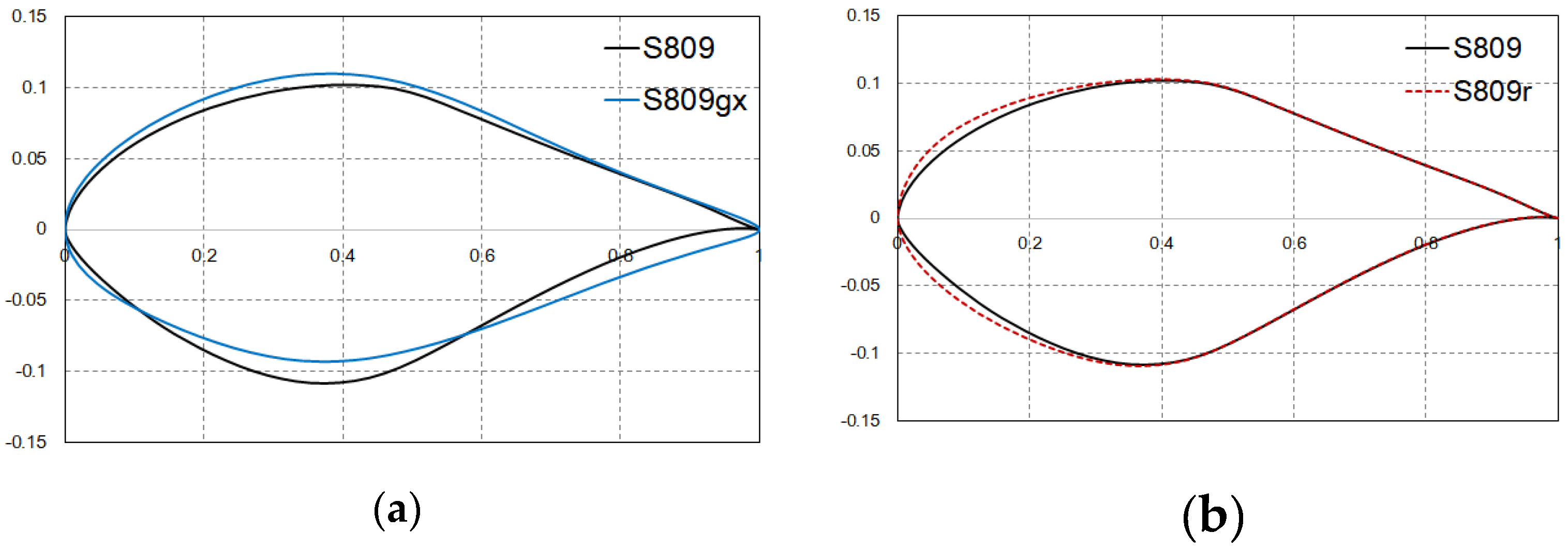
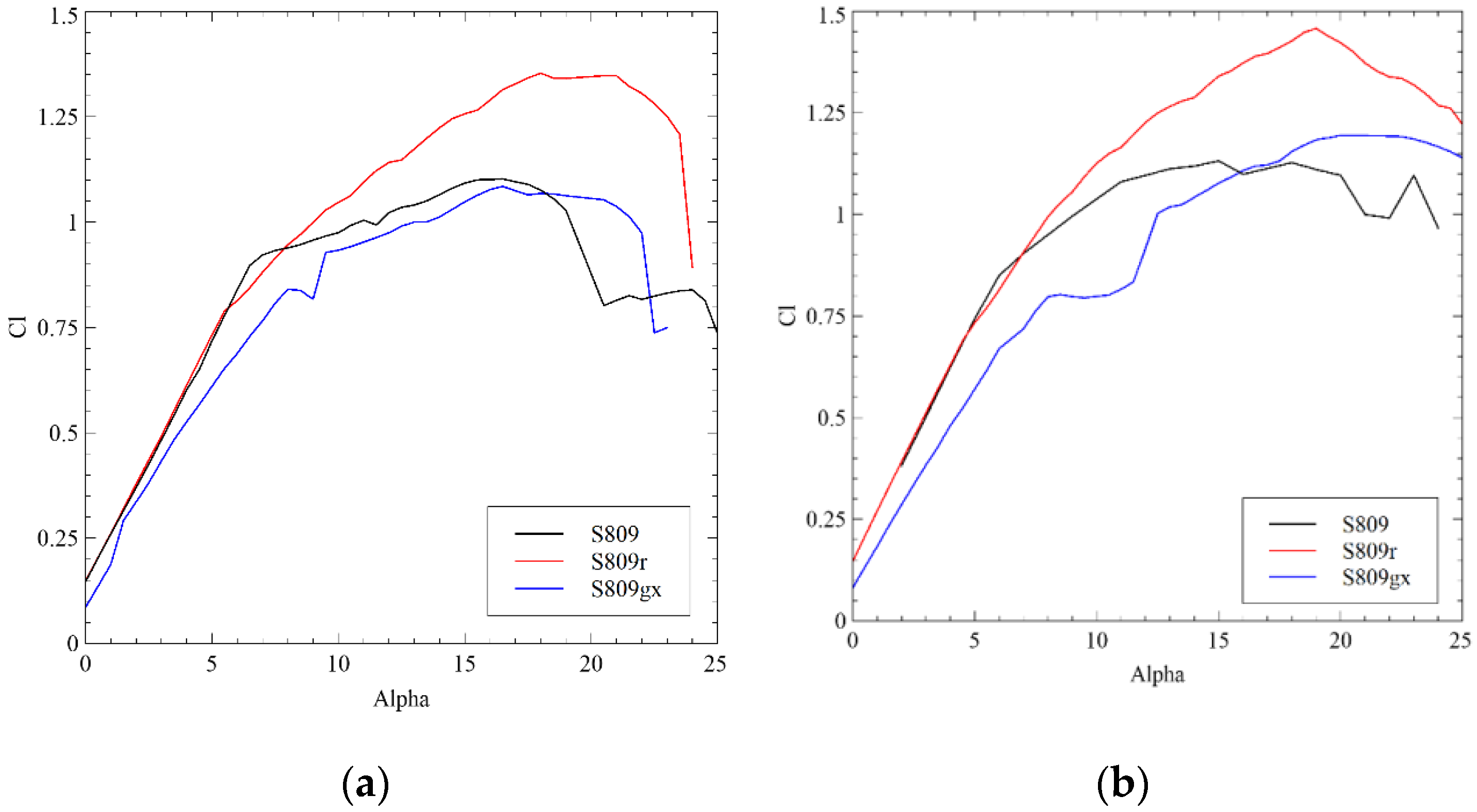
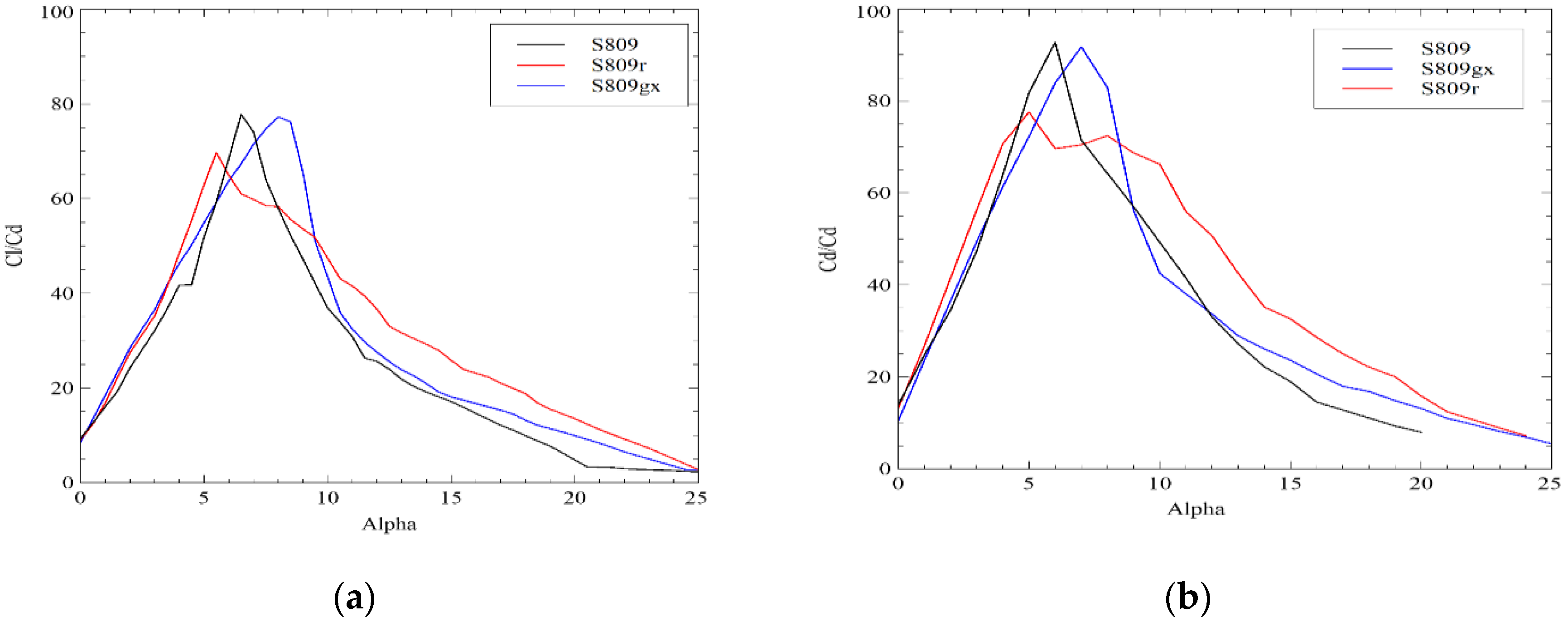
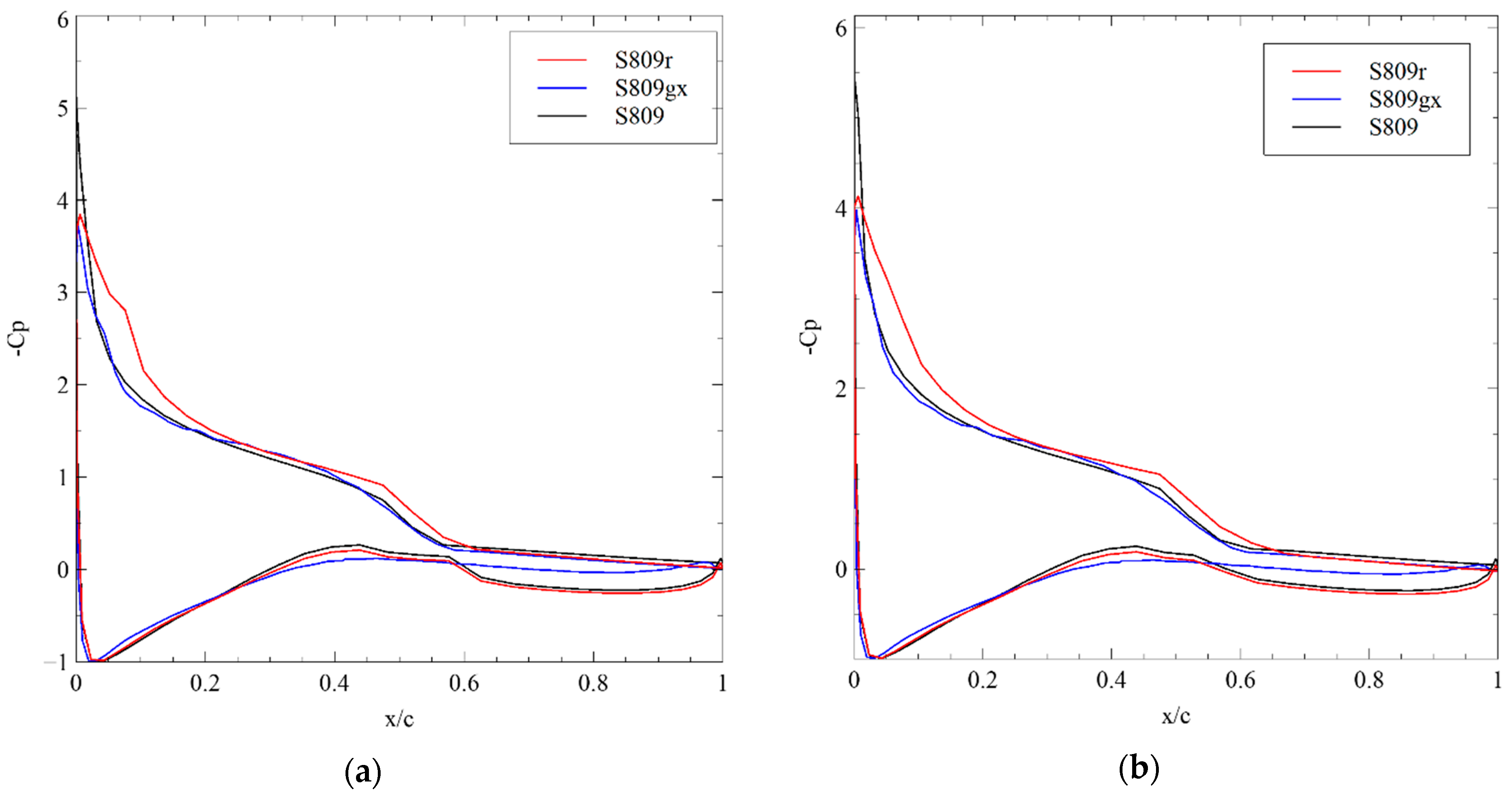
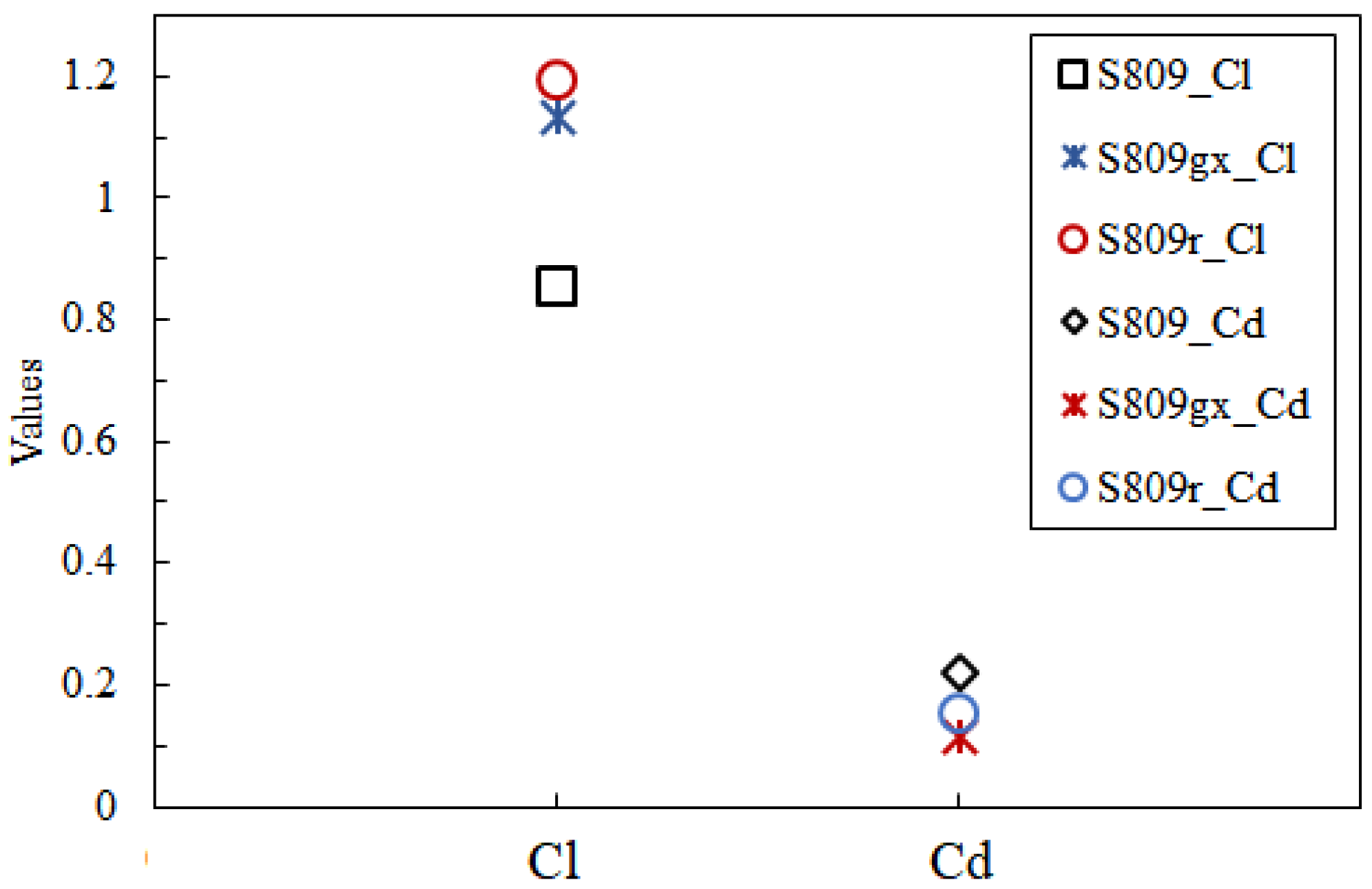
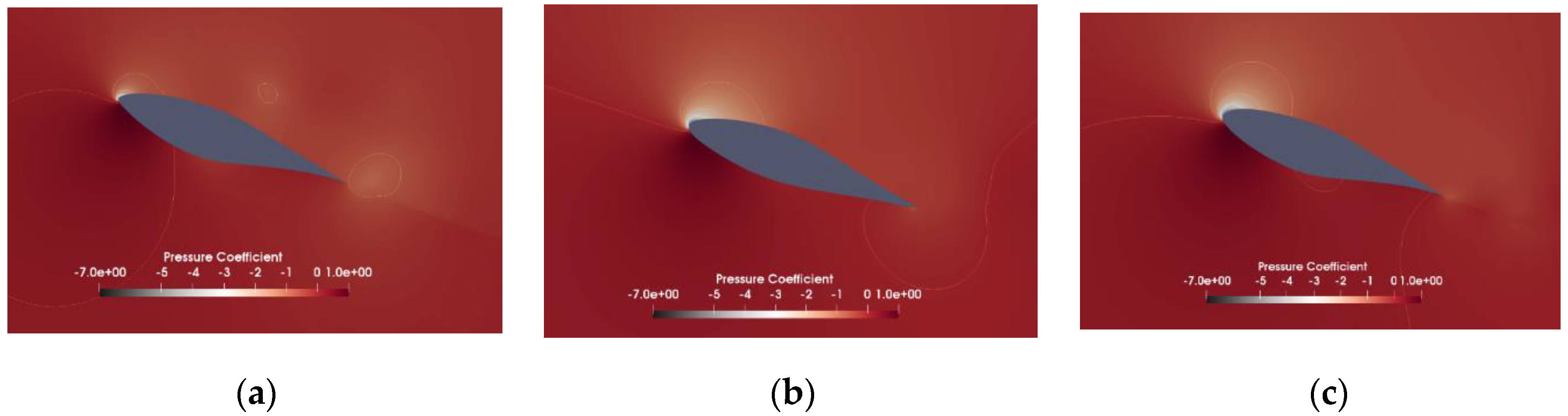
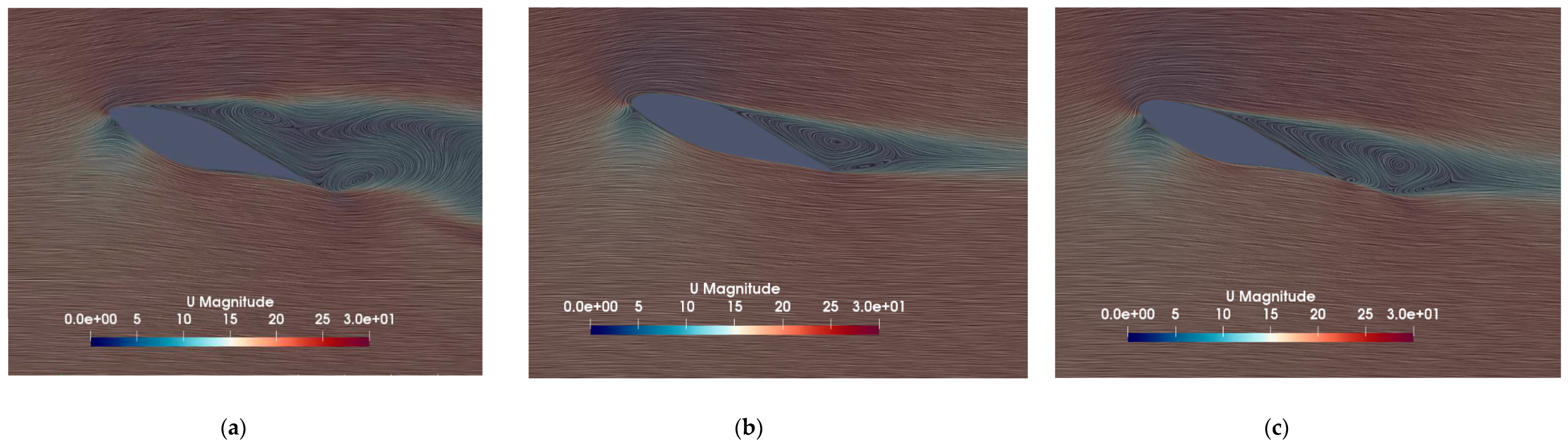
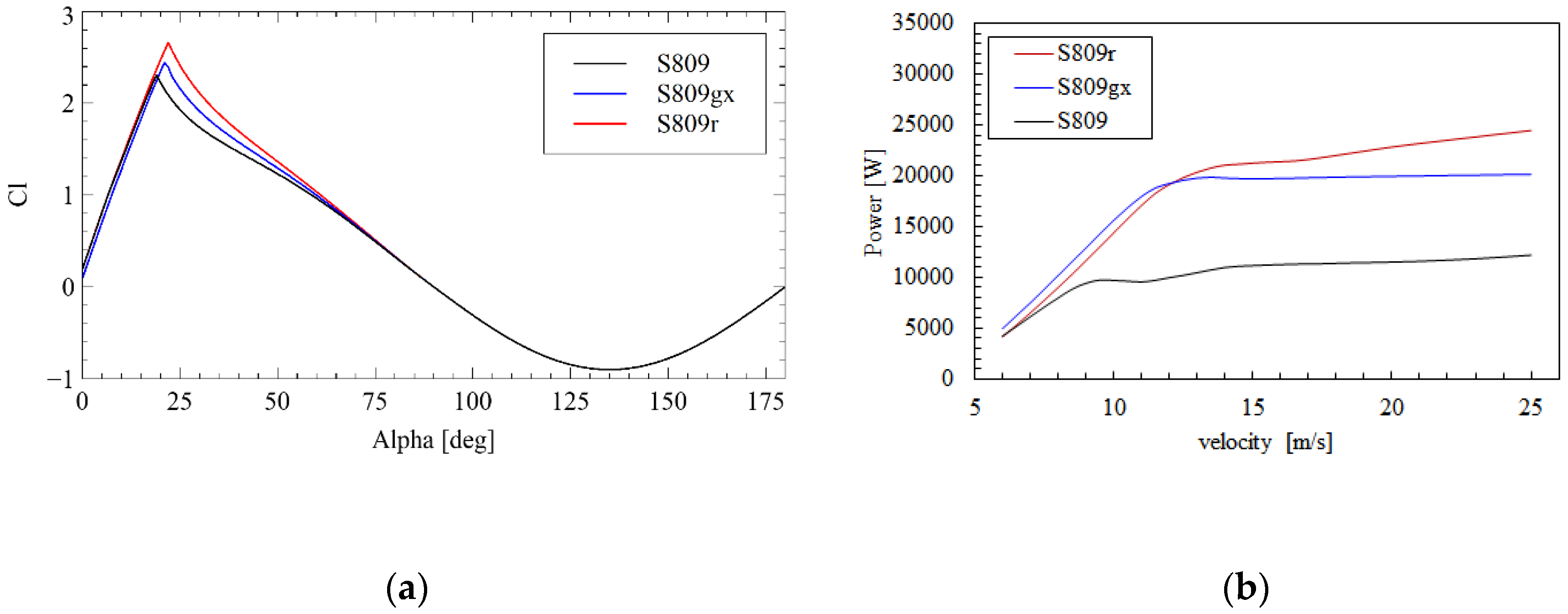
The shape differences of the airfoil S809, S809gx, and S809r show different pressure, GR distribution, transition point, lift coefficient, power production, separation, and stall area. Commonly, the GR at the fully attached range is considered the main factor in increasing power production. Therefore, the airfoil is usually designed to have the highest angle of attack at the design point. However, the airfoil S809r, which produces the highest power output in 3D correction, shows the lowest maximum GR value in the GR-alpha graph of the 2D XFOIL calculation. It shows the airfoil S809r, which has a significant improvement in lift coefficient by 360-degree extrapolation, led its highest power production. The higher lift coefficient region is mainly from the higher angle of attack, where the airfoil S809r shows the higher GR value from XFOIL. The CFD simulations of the three blade sections show that the leading-edge roundness of the airfoil influences the pressure gradients over the upper surface, which causes the less trailing edge vortex. The rounded nose impact is more significant than the trailing edge sharpness for the separation at stall alpha.

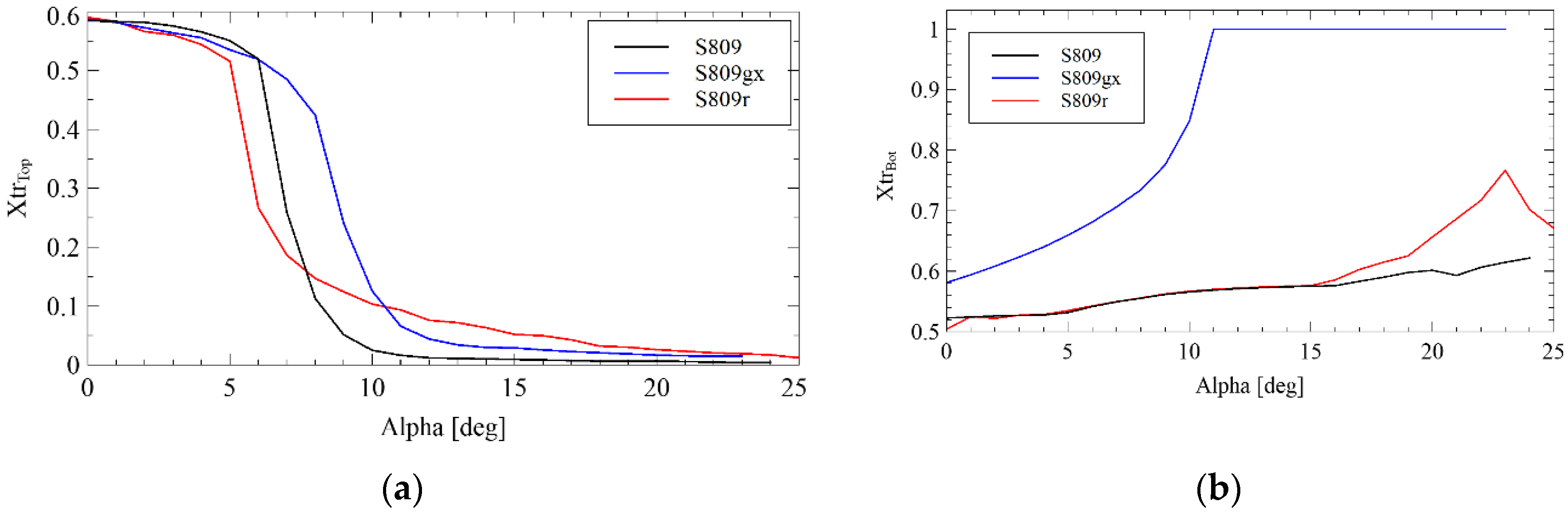
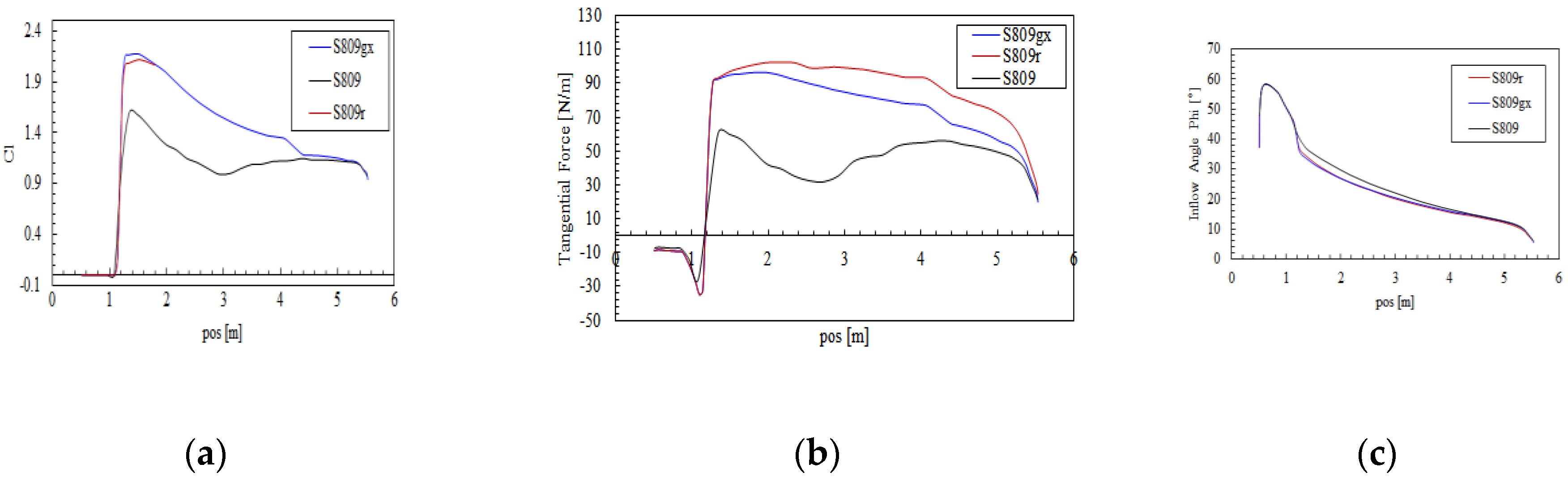
The rounded nose and the S-shaped trailing of the S809r show higher tolerance at the stall. It is in contrast to the dramatically decreased GR values of the reference airfoil at the stall alpha region. At the higher angle of attack, the airfoil S809r has an extensive laminar boundary layer. The delayed transition from laminar to turbulent flow at the S809r with the enhancement of 3D rotational flow causes less separation and stall area of the airfoil compared to the reference. The upper surface laminar region is more influential than the lower surface boundary layer. As the more laminar boundary layer at the higher angle of attack enhanced by the rotational augmentation reduces the laminar separation bubble, the lift coefficient and tangential force from the blade with the S809r show the highest lift coefficient and tangential force.

The shape difference of airfoils makes the lift, drag coefficients, and inflow angle of attack different at the same incoming velocity. The airfoil shape with increased lift and decreased drag considered with the specific incoming flow angle make a significant increase in torque. It is under sine and cosine function of normal and tangential equations that lead the desired power production by the specially shaped blades’ airfoil. These findings make the airfoil shape with reduced separation and stall at higher alpha to achieve aerodynamic performance.

The stall and separation reductions at the airfoil S809r are related to the airfoil shape, making the higher GR at the higher angle of attack region, rather than the airfoil with the highest peak the GR graph. The pressure distribution over the upper surface generated by the more rounded leading edge and symmetric airfoil geometry is connected to the blade’s aerodynamic performance and structurally stable wind turbine power production. It gives the airfoil designer insight to increase the rotor’s stable aerodynamic efficiency with the smallest cost to change the design. Further research to find another critical area of airfoil shape which influences the 3D rotational augmentation would enhance the link between the airfoil design and its impact on HAWT’s rotor aerodynamic performance.

References

1. International Renewable Energy Agency. “Trends in Renewable Energy”. Available online: https://www.irena.org/Statistics/View-Data-by-Topic/Capacity-and-Generation/Statistics-Time-Series (accessed on 30 May 2020).
2. Tangler, J.L.; Somers, D.M. NREL Airfoil Families for HAWTs; National Renewable Energy Laboratory: Washington, DC, USA, 1995; pp. 117–123.
3. Timmer, W.A.; van Rooij, R.P.J.O.M. Summary of the Delft University Wind Turbine Dedicated Airfoils. In Proceedings of the ASME 2003 Wind Energy Symposium, Reno, NV, USA, 6–9 January 2003; pp. 11–21. [Google Scholar]
4. Jianhua, X.; Zhonghua, H.; Xiaochao, Y.; Wenping, S. Design Optimization of a Multi-Megawatt Wind Turbine Blade with the NPU-MWA Airfoil Family. Energies 2019, 12, 3330. [Google Scholar]
5. Fuglsang, P.; Bak, C. Design and verification of the new Riso-A1 airfoil family for wind turbines. In Proceedings of the 20th 2001 ASME Wind Energy Symposium, Reno, NV, USA, 11–14 January 2001; pp. 81–91. [Google Scholar] [CrossRef]
6. Manwell, J.F.; McGowan, J.G.; Rogers, A.L. Wind Energy Explained; Wiley: Hoboken, NJ, USA, 2009; pp. 117–129. [Google Scholar]
7. Dev Rajnarayan, A. Ning, Universal Airfoil Parameterization Using B-Splines. In Proceedings of the AIAA Multidisciplinary Analysis and Optimization Conference, Atlanta, GA, USA, 25–29 June 2018; p. 4. [Google Scholar]
8. Chen, X.; Agarwal, R. Optimization of Flatback Airfoils for Wind Turbine Blades Using a Genetic Algorithm with an Artificial Neural Network. In Proceedings of the 48th AIAA Aerospace Sciences Meeting Including the New Horizons Forum and Aerospace Exposition, Orlando, FL, USA, 4–7 January 2010; pp. 4–7. [Google Scholar] [CrossRef]
9. Ribeiro, A.F.P.; Awruch, A.M.; Gomes, H.M. An airfoil optimization technique for wind turbines. Appl. Math. Model. 2012, 36, 4898–4907. [Google Scholar] [CrossRef]
10. Michael, S. Airfoil Design Using A Genetic Algorithm and an Inverse Method. In Proceedings of the 41st Aerospace Sciences Meeting and Exhibit, Reno, Nevada, USA, 6–9 January 2003. [Google Scholar]
11. Ronsten, G. Static pressure measurements on a rotating and a non-rotating 2.375 m wind turbine blade. Comparison with 2D calculations. J. Wind. Eng. Ind. Aerodyn. 1992, 39, 105–118. [Google Scholar] [CrossRef]
12. XFOIL, Subsonic Airfoil Development System. Available online: https://web.mit.edu/drela/Public/web/xfoil/ (accessed on 30 May 2020).
13. Himmelskamp, H. Profile Investigation on a Rotating Airscrew, Technical Report. Ph.D. Thesis, University of Göttingen, Göttingen, Germany, 1945. [Google Scholar]
14. Bruining, A.; Van Bussel, G.J.W.; Corten, G.P.; Timmer, W.A. Pressure Distribution from a Wind Turbine Blade; Field Measurements Compared to 2-Dimensional Wind Tunnel Data; Technical Report IW-93065R; Delft University of Technology: Delft, The Netherland, 1993. [Google Scholar]
15. Liu, F.; Gao, S.; Liu, D.; Zhou, H. A signal decomposition method based on repeated extraction of maximum energy component for offshore structures. Mar. Struct. 2020, 72, 102779. [Google Scholar] [CrossRef]
16. Gersten, S. Boundary Layer Theory; Springer: Berlin/Heidelberg, Germany, 2017. [Google Scholar]
17. Herrmann, J.; Bangga, G. Multi-objective optimization of a thick blade root airfoil to improve the energy production of large wind turbines. J. Renew. Sustain. Energy 2019, 11, 043304. [Google Scholar] [CrossRef]
18. Chaviaropoulos, P.K.; Hansen, M.O. Investigating Three-Dimensional and Rotational Effects on Wind Turbine Blades by Means of a Quasi-3D Navier-Stokes Solver. J. Fluids Eng. 2000, 122, 330–336. [Google Scholar] [CrossRef]
19. Mirzaei, M.; Roshanian, J.; Nasrin Hosseini, S. Aerodynamic optimization of an airfoil using gradient based method. In European Conference on Computational Fluid Dynamics; ECCOMAS CFD: TU Delft, Delft, The Netherland, 2006. [Google Scholar]
20. Bangga, G.; Lutz, T.; Jost, E.; Krämer, E. CFD studies on rotational augmentation at the inboard sections of a 10 MW wind turbine rotor. J. Renew. Sustain. Energy 2017, 9, 023304. [Google Scholar] [CrossRef]
21. Hansen, M.O.; Sorensen, J.; Michelsen, J.; Sørensen, N.N. A Global Navier-Stokes Rotor Prediction Model. In Proceedings of the 35th Aerospace Sciences Meeting and Exhibit, Reno, NV, USA, 6–9 January 1997. [Google Scholar] [CrossRef]
22. Snel, H.; Houwink, R.; Piers, W.J. Sectional Prediction of 3-D Effects for Separated Flow on Rotating Blades. In Proceedings of the Eighteenth European Rotorcraft Forum, Avignon, France, 15–17 September 1992. Chapter 6 References 133. [Google Scholar]
23. Snel, H.; Houwink, R.; Bosschers, J.; Piers, W.J.; Bruining, A. Sectional Prediction of 3-D Effects for Stalled Flows on Rotating Blades and Comparison with Measurements. In Proceedings of the ECWEC ’93 Conference, Travemunde, Germany, 8–12 March 1993; pp. 395–399. [Google Scholar]
24. Hand, M.M.; Simms, D.; Fingersh, L.J.; Jager, D.W.; Cotrell, J.R.; Schreck, S.; Larwood, S.M. Unsteady Aerodynamics Experiment Phase VI: Wind Tunnel Test Configurations and Available Data Campaigns; (No. NREL/TP-500-29955); National Renewable Energy Lab.: Golden, CO, USA, 2001.
25. Berry, D.S.; Composites, D.S. Blade System Design Studies Phase II: Final Project Report; SANDIA: Oak Ridge, TN, USA, 2008.
26. NASA Aeronautics Guided Tour. Available online: https://www.grc.nasa.gov/WWW/k-12/airplane/incline.html (accessed on 5 August 2020).
27. Bangga, G.; Lutz, T.; Krämer, E. Numerical Investigation of Unsteady Aerodynamic Effects on Thick Flatback Airfoils; German Wind Energy Conference: Bremen, Germany, 2015; p. 12. [Google Scholar]
28. Somers, D.M. Design and Experimental Results for the S809 Airfoil; NREL: Golden, CO, USA, 1997.
29. Cheney, E.W.; Kincaid, D.R. Numerical Mathematics and Computing, 6th ed.; Brooks Cole: Pacific Grove, CA, USA, 2007; pp. 372–404. [Google Scholar]
30. Breton, S.-P.; Coton, F.N.; Moe, G. A study on rotational effects and different stall delay models using a prescribed wake vortex scheme and NREL phase VI experiment data. Wind. Energy 2008, 11, 459–482. [Google Scholar] [CrossRef]
31. Kim, Y. Genetic Algorithm Optimization of Variable Airfoil Blade of Wind Turbines. Master’s Thesis, Institute of Fluid Mechanics (LSTM), FAU Erlangen-Nuernberg, Erlangen, Germany, 2014. [Google Scholar]
32. Kim, Y.; Al-Abadi, A.; Delgado, A. Airfoil Boundary Layer Optimization Toward Aerodynamic Efficiency of Wind Turbines. In Flight Physics—Models, Techniques and Technologies; IntechOpen: London, UK, 2018. [Google Scholar]
33. Kim, Y. Computational Airfoil Optimization for the Improvement of the Performance of Horizontal Axis Wind Turbine (HAWT) with a 3D Model. Doctor’s Thesis, Institute of Fluid Mechanics (LSTM), FAU Erlangen-Nuernberg, Erlangen-Nuernberg, Erlangen, Germany, 2020. [Google Scholar]
34. Drela, M. XFOIL: An Analysis and Design System for Low Reynolds Number Airfoils. In Multiphase Flow in Porous Media; Springer Science and Business Media LLC: Berlin, Germany, 1989; pp. 1–12. [Google Scholar]
35. Zhang, W.; Cheng, W.; Gao, W.; Qamar, A.; Samtaney, R. Geometrical effects on the airfoil flow separation and transition. Comput. Fluids 2015, 116, 60–73. [Google Scholar] [CrossRef] [Green Version]
36. Ramsay, R.; Hoffman, M.; Gregorek, G. Effects of Grit Roughness and Pitch Oscillations on the S809 Airfoil; National Renewable Energy Lab.: Golden, CO, USA, 1995.
37. Timmer, W.A.; Van Rooij, R.P.J.O.M. Summary of the Delft University Wind Turbine Dedicated Airfoils. J. Sol. Energy Eng. 2003, 125, 488–496. [Google Scholar] [CrossRef]
38. Johnson, W. Rotorcraft Aeromechanics; Cambridge University Press: Cambridge, UK, 2013. [Google Scholar]
39. Ingram, G. Wind Turbine Blade Analysis Using the Blade Element Momentum Method Version 1.0; School of Engineering, Durham University: Durham, UK, 2005. [Google Scholar]
40. Kim, Y.; Bangga, G.; Delgado, A. Wind Turbine Airfoil Boundary Layer Optimization Using Genetic Algorithm with 3D Rotational Augmentation. In Design Optimization of Wind Energy Conversion Systems with Applications; IntechOpen: London, UK, 2020. [Google Scholar]
41. Viterna, L.A.; Janetzke, D.C. Theoretical and Experimental Power from Large Horizontal-Axis Wind Turbines; National Aeronautics and Space Administration: Cleveland, OH, USA, 1982.
42. Qblade, Wind Turbine Design and Simulation. Available online: http://www.q-blade.org/ (accessed on 6 August 2020).
43. SimFlow. Weighing up the options for sound testing methods. Met. Powder Rep. 2008, 63, 11. [Google Scholar] [CrossRef]
44. Zhou, D.; Liu, Y.; Wen, X.; Lu, L. Modification of SA model for predicting airfoil flow separation. J. Beijing Univ. Aeronaut. Astronaut. 2012, 38, 1384–1388. [Google Scholar]
45. Guerri, O.; Bouhadef, K.; Harhad, A. Turbulent Flow Simulation of the NREL S809 Airfoil. Wind. Eng. 2006, 30, 287–301. [Google Scholar] [CrossRef]
46. Shelton, A.; Abras, J.; Jurenko, R.; Smith, M. Improving the CFD Predictions of Airfoils in Stall. In Proceedings of the 43rd AIAA Aerospace Sciences Meeting and Exhibit, Reno, NV, USA, 10–13 January 2005. [Google Scholar] [CrossRef]
47. Menter, F.R. Two-equation eddy-viscosity turbulence models for engineering applications. Aiaa J. 1994, 32, 1598–1605. [Google Scholar] [CrossRef] [Green Version]
48. The Open Source CFD Toolbox. Available online: https://www.openfoam.com/ (accessed on 13 June 2020).
49. Liu, F.; Gao, S.; Tian, Z.; Liu, D. A new time-frequency analysis method based on single mode function decomposition for offshore wind turbines. Mar. Struct. 2020, 72, 102782. [Google Scholar] [CrossRef]
50. Moukalled, F.; Mangani, L.; Darwish, M. An Advanced Introduction with OpenFOAM® and Matlab; Springer: Cham, Switzerland, 2006. [Google Scholar]
51. Lindenburg, C. Investigation into Rotor Blade Aerodynamics; ECN: Sint Maartensvlotbrug, The Netherland, 2003. [Google Scholar]
52. Van der Hegge Zijnen, B.G. Measurements of the Velocity Distribution in the Boundary Layer along a Plane Surface. Ph.D. Thesis, Technical University of Delft, Delft, The Netherland, 1924. [Google Scholar]
53. Li, Y.; Paik, K.-J.; Xing, T.; Carrica, P.M. Dynamic overset CFD simulations of wind turbine aerodynamics. Renew. Energy 2012, 37, 285–298. [Google Scholar] [CrossRef]
Figure 1. Representation of the general airfoil shape discretization using B-spline curve.
Sustainability 12 07597 g001
Figure 2. The airfoil shapes of (a) airfoil S809, S809gx, (b) airfoil S809, S809r.
Sustainability 12 07597 g002
Figure 3. Illustration of the blade designs with airfoils:(a) S809, (b) S809gx, (c) S809r.
Sustainability 12 07597 g003
Figure 4. Rotating cross-section at different position 1–4 [39].
Sustainability 12 07597 g004
Figure 5. Rotor radial elements.
Sustainability 12 07597 g005
Figure 6. Velocity triangle at a blade section.
Sustainability 12 07597 g006
Figure 7. Three different airfoils with similar thickness: (a) reference S809, (b) rounded nose and symmetric airfoil S809gx, (c) rounded nose airfoil S809r.
Sustainability 12 07597 g007
Figure 8. Overall view of the computational domain.
Sustainability 12 07597 g008
Figure 9. Computational grid of the airfoil (S809).
Sustainability 12 07597 g009
Figure 10. (a) Pressure coefficients of S809 at Re = 10 6 alpha = 12.2° from XFOIL and experimental data (Exp) [36], (b) CFD and Exp at Re = 1.5   ×   10 6 alpha = 12.2°, (c) XFOIL and Exp at Re = 1.5   ×   10 6 , alpha = 20.2°, (d) CFD and Exp at Re = 1.5   ×   10 6 , alpha = 20.2°.
Sustainability 12 07597 g010aSustainability 12 07597 g010b
Figure 11. Computed lift and drag coefficients predicted using XFOIL in comparison with the Exp [28].
Sustainability 12 07597 g011
Figure 12. Predicted transition points at the (a) upper, (b) lower parts of the airfoil at various angles of attack in comparison with Exp [28].
Sustainability 12 07597 g012
Figure 13. Lift coefficient by 3D correction law and extracted 3D Exp [51].
Sustainability 12 07597 g013
Figure 14. Power curve predicted using 3D-corrected BEM in comparison with Exp [51,53].
Sustainability 12 07597 g014
Figure 15. Lift coefficient of three airfoils at (a) Re = 0.55   ×   10 6 , (b) Re = 10 6 without applying 3D correction law.
Sustainability 12 07597 g015
Figure 16. Drag coefficient of three airfoils at (a) Re = 0.55   ×   10 6 , (b) Re = 10 6 without applying 3D correction law.
Sustainability 12 07597 g016
Figure 17. Gliding ratio of three airfoils at (a) Re = 0.55   ×   10 6 , (b) Re = 10 6 without applying 3D.
Sustainability 12 07597 g017
Figure 18. Pressure coefficient of three airfoils at (a) Re = 0.55   ×   10 6 , (b) Re = 10 6 without applying 3D correction law.
Sustainability 12 07597 g018
Figure 19. Airfoil S809 (a) Cl and (b) Cd values at alpha=12.2° and 20° from OpenFoam and experiment [36].
Sustainability 12 07597 g019
Figure 20. Airfoil S809, S809gx, and S809r C17-18l and Cd values at alpha = 20° from OpenFoam.
Sustainability 12 07597 g020
Figure 21. Contour of the pressure coefficients of at Re = 1.5   ×   10 6 alpha = 20.2° for (a) S809, (b) S809gx, (c) S809r.
Sustainability 12 07597 g021
Figure 22. Contour of velocity magnitude of at Re = 1.5   ×   10 6 alpha = 20.2° for (a) S809, (b) S809gx, (c) S809r.
Sustainability 12 07597 g022
Figure 23. (a) Transition point (Xtr) at top, (b) transition point (Xtr) at bottom at Re = 10 6 .
Sustainability 12 07597 g023
Figure 24. (a) Extrapolated lift coefficient at Re = 0.55   ×   10 6 , (b) power production.
Sustainability 12 07597 g024
Figure 25. (a) Lift coefficient at the blade position, (b) tangential force, (c) inflow angle at v = 10 m/s.
Sustainability 12 07597 g025