A Data-Driven Approach to Trip Generation Modeling for Urban Residents and Non-local Travelers


1
Jiangsu Key Laboratory of Urban ITS, Jiangsu Province Collaborative Innovation Center of Modern Urban Traffic Technologies, School of Transportation, Southeast University, Nanjing 211189, China
2
College of Civil and Transportation Engineering, Shenzhen University, Shenzhen 518060, China
*
Author to whom correspondence should be addressed.
Sustainability 2020, 12(18), 7688; https://0-doi-org.brum.beds.ac.uk/10.3390/su12187688
Submission received: 21 August 2020
/
Revised: 14 September 2020
/
Accepted: 14 September 2020
/
Published: 17 September 2020
(This article belongs to the Collection Sustainability in Urban Transportation Planning)
Abstract
:Trip generation modeling is essential in transportation planning activities. Previous modeling methods that depend on traditional data collection methods are inefficient and expensive. This paper proposed a novel data-driven trip generation modeling method for urban residents and non-local travelers utilizing location-based social network (LBSN) data and cellular phone data and conducted a case study in Nanjing, China. First, the point of interest (POI) data of the LBSN were classified into various categories by the service type, then, four features of each category including the number of users, number of POIs, number of check-ins, and number of photos were aggregated by traffic analysis zones to be used as explanatory variables for the trip generation models. We used a random tree regression method to select the most important features as the model inputs, and the trip models were established based on the ordinary least square model. Then, an exploratory approach was used to test the performance of each combination of the variables with various test methods to identify the best model for residents’ and travelers’ trip generation functions. The results suggest land use compositions have significant impact on trip generations, and the trip generation patterns are different between urban residents and non-local travelers.
1. Introduction
Trip generation modeling is the first step in the traditional travel demand forecasting procedure, and it is integral in evaluating the transportation impacts of land use developments. In transportation planning activities, the cities are divided into various traffic analysis zones (TAZs). The trip generation models aim to predict the total number of trips generated and attracted to each TAZ. Transportation planning agencies need to collect the travel survey data, land use data, and socio-economic data to implement the calculation of the trip generation models [1]. Traditional methods to acquire these data are expensive and inefficient since a significant number of trained staff are required to collect trip data from residents of various family sizes and income levels [2,3]. Moreover, the non-local travelers are often neglected during the in-house survey procedure. However, with the development of urban cities, the connections and trip exchanges between urban major cities become more frequent. The non-local traveler trips contribute an increasing fraction of the total trips in the city. In addition, existing research has found that the non-local travelers’ trips are different from residents’ trips in terms of trip length distributions, trip purposes, and trip frequencies [4]. New, effective trip survey methods are required to construct more accurate and effective trip generation models for both residents and non-local travelers.
Recent research on transportation planning, especially trip generation forecasting, explored various methods to collect travel data, including global positioning system (GPS) data, cellular service data, and location-based social network (LBSN) data. The GPS data can provide trip makers’ travel trajectories with high spatial accuracy. Researchers have used GPS data to obtain real-time traffic status on roadway segments [5] and to construct personal users’ travel choice recommendation systems [6], however, GPS data are rarely used to analyze travel patterns on a large scale at a city level since users may not use navigation services for every trip, especially for their routine commuting trips, therefore, the GPS technique has a deficiency in collecting data of a sufficiently large sample size. The cellular phone data can provide trip information of a large population size, including for both residents and travelers with high temporal and spatial resolution. Previous research utilized cellular phone data to obtain travel information of a large population size for various transportation studies such as origin–destination matrix estimation [7,8], traffic status monitoring [9,10], travel behavior analysis [11] etc. The disadvantage of cellular phone data is that they do not include the purpose of users’ travel activities and the information of users’ personal social and economic attributes. In LBSN services, locations in the real world are labeled by service providers and users with specific service types such as office, residence, food, etc., which constitutes the points of interest (POIs) of the LBSN. Users check-in at different POIs by sharing their locations and comments with their friends, creating abundant trajectory records. The LBSN data can provide an inexpensive and convenient data source for quantifying the strength of trip activity in an area and inferring land use type by the most popular activity type. The transportation researchers have demonstrated the advantages of LBSN data in various applications [12]. Some research utilized the check-ins of the LBSN data to estimate trip demand [3,13,14]: one research paper used Foursquare check-in data to estimate the Origin Destination matrix for non-commuting trips [14], and another research paper utilized check-in data to estimate trip demand for shared-bikes [13]. In urban cities, many areas have compound service types. The POIs in the LBSN data have the advantage of describing the land use type and quantify the fraction of different service types. Some research focused on utilizing the service types of the POI data in the LBSN [15,16,17,18]: one research paper proposed a trip purpose inference method using POI service type compositions in the destination area [17], one research paper used the POI data to identify the land use type of city blocks [18], and another research paper identified the correlation between roadway traffic flow and built-in environments [16].
In conclusion, combining the advantages of the cellular phone data and those of the LBSN data could provide new opportunities to c new trip generation models with better accuracy and at low cost. The cellular phone data could be used to calculate the number of trips produced and attractions of urban residents and non-local travelers. The LBSN data, which includes the POI type and check-in number, could be used as variables suggesting land use and attractiveness of trips. With the cellular phone data and LBSN data combined, we can explore the relationship between trip production and attraction and different POI types in a traffic analysis zone. For future trip generation estimation with new land use developments, reasonable prediction of trip production/attraction of urban residents and non-local travelers could be calculated using the LBSN data.
This paper aimed to propose a novel trip generation modeling method using LBSN data and cellular phone data for both residents and travelers in urban cities. The rest of the paper is organized as follows: Section 2 introduces the data sets used in this research and presents some preliminary data analysis; Section 3 introduces the procedures of the methodology, including four steps: feature selection, exploratory approach to building trip models, model selection, and model evaluation; Section 4 describes a case study conducted in Nanjing and analyzes the results. Section 5 concludes the paper.
2. Data
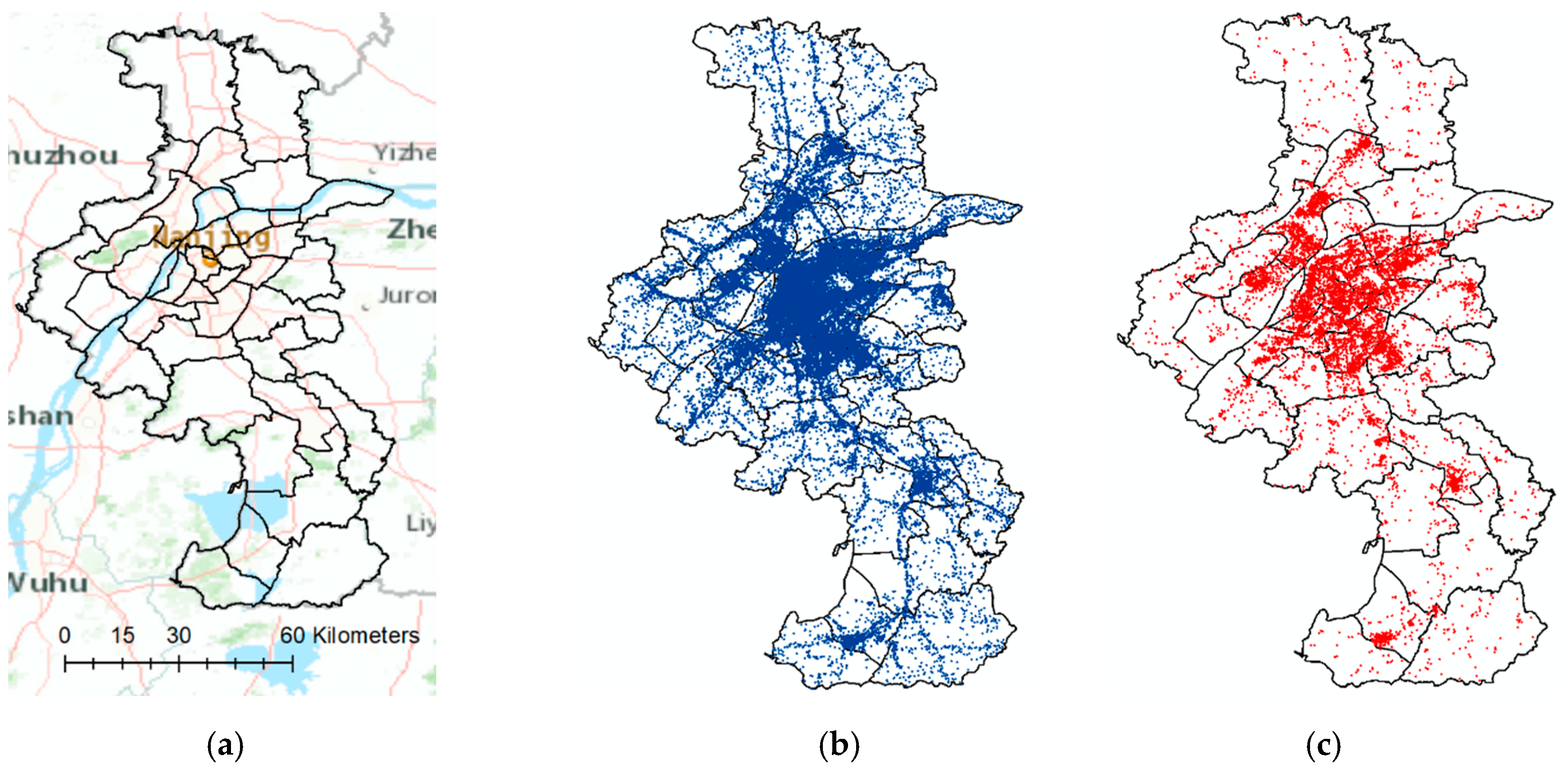
This study was conducted in the city of Nanjing in China, which is an urban metropolitan area with a population size of 8.27 million [19]. The area of the city is approximately 6587 km2 [19]. The city is divided into 11 administrative zones and 38 traffic analysis zones (TAZs) by the transportation management department. Figure 1a illustrates the research area with the TAZ divisions. In the central area where the population is densely distributed, the TAZs are relatively small compared with the TAZs in the suburban area where the population is less densely distributed. Figure 1b presents the spatial distribution of the 77,061 cellular signal base stations in Nanjing. Figure 1c illustrates the spatial distribution of the 11,719 points of interest (POI) of a location-based social network (LBSN) service. The LBSN data were collected from Weibo, which is one of the most popular social service providers in China with over 465 million active users nationwide as of 2019 [20]. As indicated in Figure 1, both the cellular signal base stations and POIs have good spatial coverage in Nanjing. The base stations and the POIs are more densely distributed in the central area and less distributed in the suburban area.
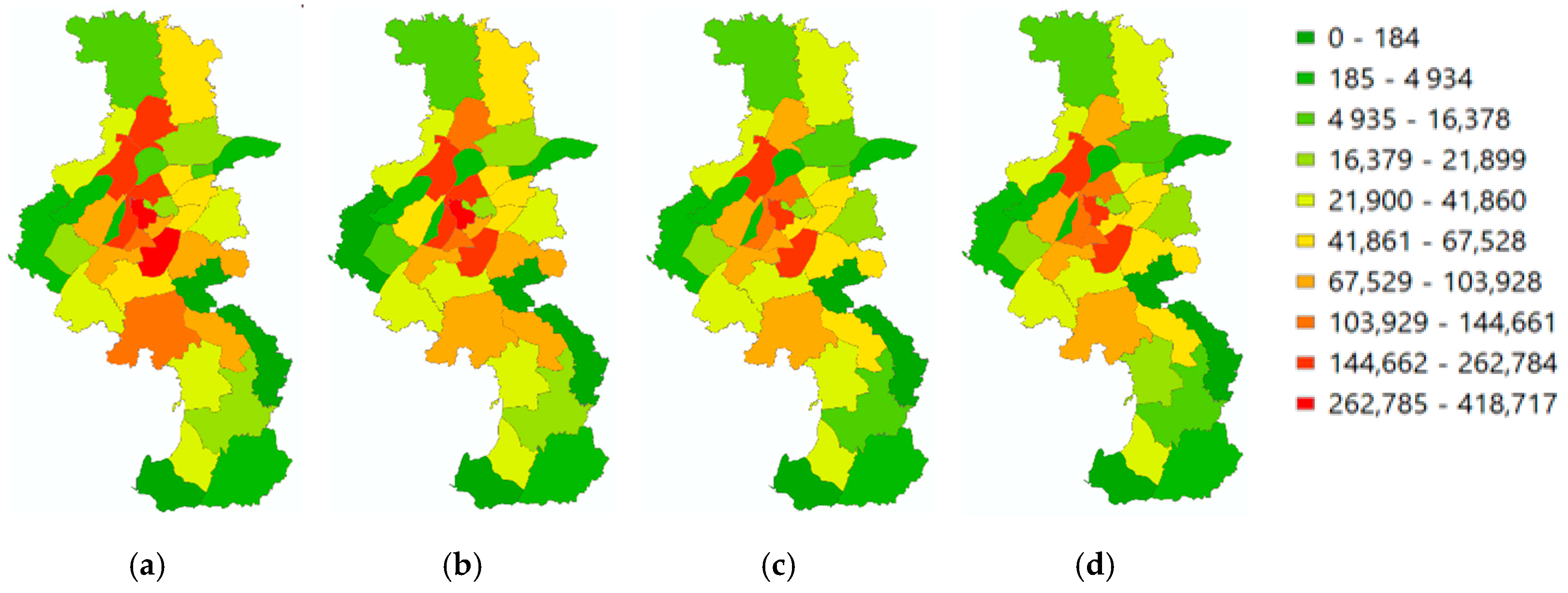
Figure 2 shows the trip productions and attractions for the residents and the travelers, which were collected from a travel survey conducted by the transportation management department using cellular phone data in February 2016. As indicated in Figure 2, most of the residents’ and travelers’ trips were generated in the central area where the population is densely distributed, while trips were fewer in the suburban area compared with the central area. There were more resident trips than traveler trips since the resident population is larger than that of travelers.
Weibo provides an application programming interface (API) [21] for collecting detailed information at each POI, including the locations, the service types, and statistics about the total check-in counts, user counts, and number of photos uploaded by users. The service types of the Weibo POI are labeled with 272 detailed categories, we further grouped these categories into 10 classifications: residence, office, entertainment, school, transportation facility, outdoor, service, food, hotel, and others. The “other” category contained POIs labeled as district names or street names, from which we cannot infer the specific service type. The user-created personal tags were also classified as other. The service types were classified as per the following list:
- Transportation Facility: Bus Stop, Subway Entrance, Parking Lot, Train Station, Inter-city Bus Station, etc.
- Residence: Residential Building, Residential District, Apartment, etc.
- Office: Office Building, Government Building, Tech Startup, Design Studio, etc.
- Entertainment: Museum, Nightclub, Bar, Theater, Club, Karaoke Club, Cinema, Memorial Hall, Exhibition Hall, Entertainment, etc.
- School: Campus, University Building, Primary School, High School, etc.
- Outdoor: Park, Historical Spot, Botanical Garden, Scenic Lookout, etc.
- Service: Mall, Supermarket, Store, Cosmetics Shop, Bookstore, Boutique, Miscellaneous Shop, etc.
- Food: Diner, Restaurant, Local Food, Coffee Shop, Pizza, Burger, Cafe, Bakery, Food, Steakhouse, Dessert Shop, etc.
- Hotel: Hotel, Inn, Guest House, etc.
- Other: User Created POI, Street Name, etc.
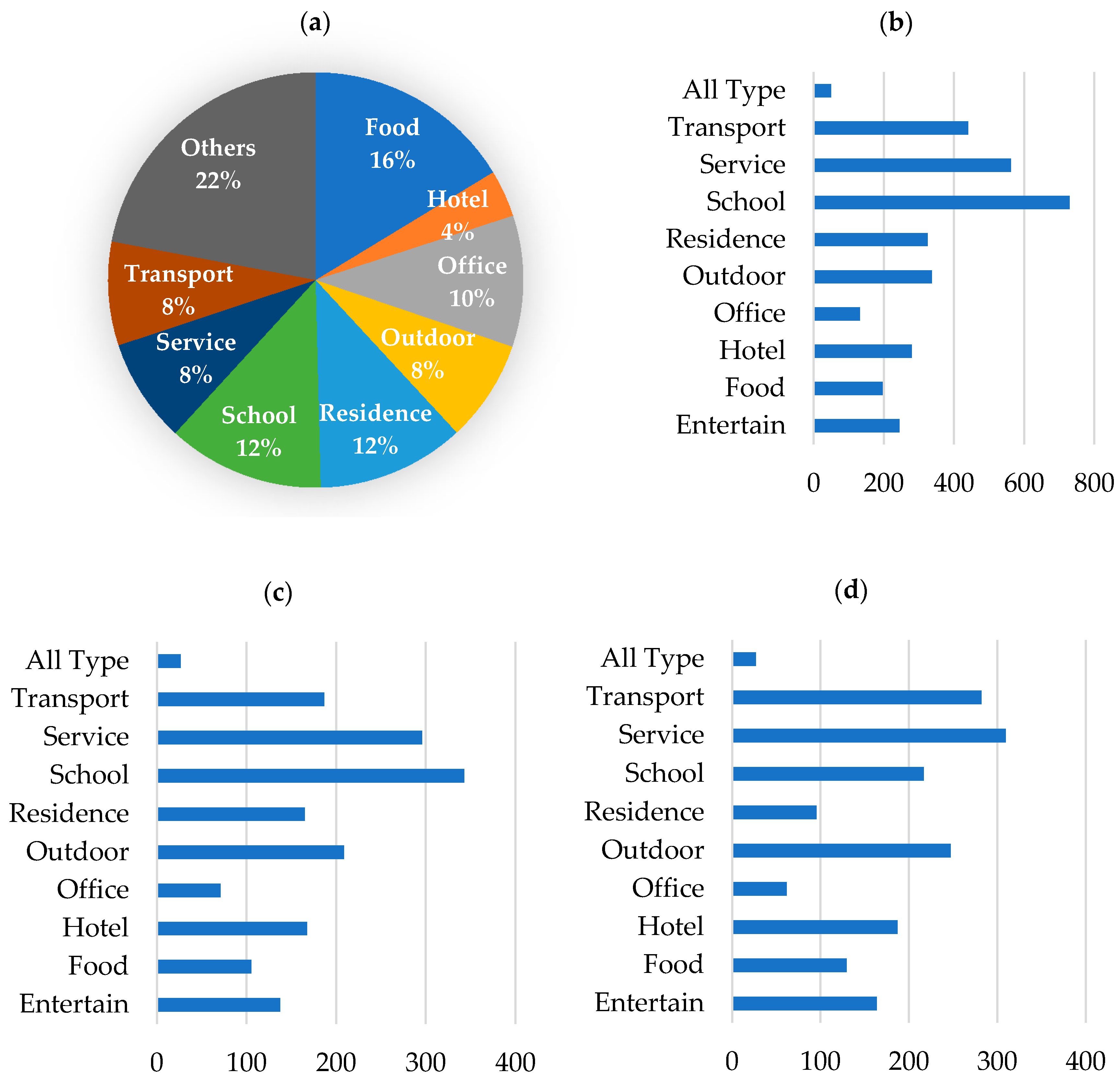
We collected the information of all the 11,719 POIs in the research area from the API. Figure 3 displays the share of POIs per category, the average check-ins per POI, the average number of photos per POI, and the average number of users per POI, which were calculated based on the historical accumulative statistics.
Figure 3a presents the details of POIs by the service type in Nanjing. The “other” POIs made up 22% of all POIs; most of them were created by users for personal use. The historical check-ins and number of users were very low compared with the POIs with a certain service type. Therefore, the “other” POI type was not considered as an explanatory variable in the trip generation model. Instead, the total number of all POIs in each TAZ was considered as an explanatory variable in the trip generating models, since the total POI number may reflect the general prosperity of the district. Figure 3b–d displays the average number of photos, check-ins, and users for the potential explanatory variables including each POI type and “all types”. The average check-in per POI and the average photos per POI had very similar patterns in POI distributions. The “school”, “service”, and “transportation facility” POIs attracted more check-ins and photo uploads. The “service”, “school”, and “outdoor” POIs attracted more users. The “school” category received the largest number of average daily check-ins while the “office” POIs received the lowest daily check-ins, which suggests that users’ preferences to check-in vary with different service type categories. Therefore, when the POI data are used as explanatory variables in trip generation models, the heterogeneity of the different POI service types should be considered.
3. Methods
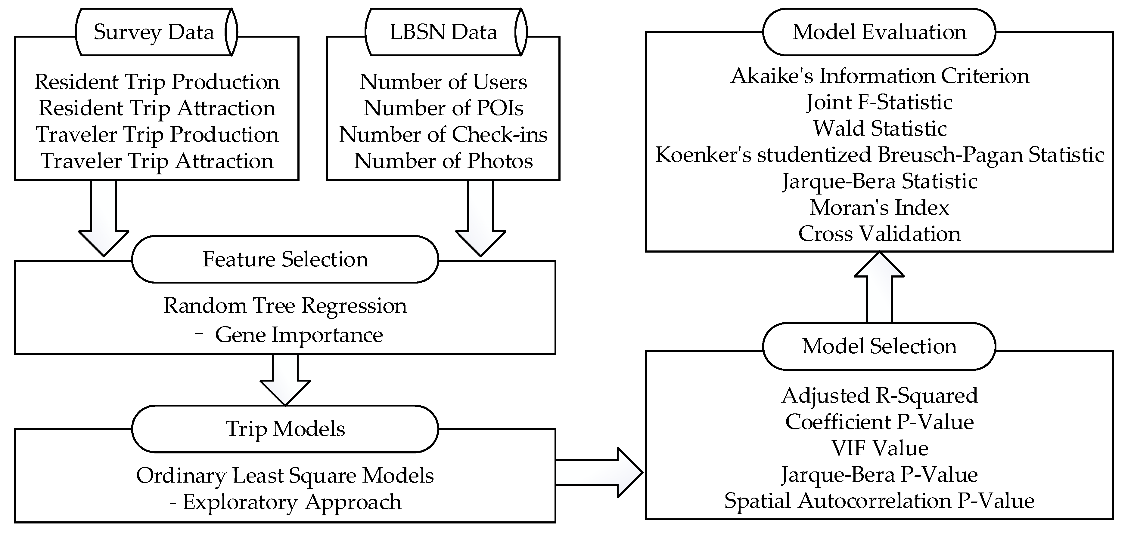
The trip generation modeling in transportation planning procedure calculates the number of trips produced and attracted by each traffic analysis zone. The data used in this research included the LBSN data, which consists of the number of POIs, number of users, number of check-ins, number of photos for each POI service type in the TAZs, and survey data, which provide trip production and attraction statistics for urban residents and non-local travelers. The survey data were provided by the transportation management department by using cellular phone data, which guarantees the quality of the data. The methodology framework of our data-driven method to model the trip generation function is shown in Figure 4, which includes four steps: feature selection, exploratory approach to building trip models, model selection, and model evaluation. The LBSN data includes four features for each traffic analysis zone, and each feature can be classified into 10 different POI categories as listed in the previous section, which formulate 40 possible factors relating to trip production or attraction. Firstly, we used the random tree regression method to evaluate the importance of the 40 explanatory variables, and selected the most important feature out of the four features. Then, we established trip models for resident trip production, resident trip attraction, traveler trip production, and traveler trip attraction based on the ordinary least square model. We used an exploratory approach to test the performances of each combination of explanatory variables. The best models were selected using five indicators: the adjusted R-squared value, and the p-value, the variance inflation factor (VIF) value, the Jarque–Bera p-value, and the spatial autocorrelation p-value for each coefficient. The performances of the selected models were evaluated using Akaike’s information criterion, joint F-statistic, Wald statistic, Koenker’s studentized Breusch–Pagan statistic, Jarque–Bera statistic, and the Moran’s index method to validate the robustness of the models.
3.1. Feature Selection Using Random Forest Regression Method
In this study, the random forest regression method was employed to evaluate the importance of each LBSN feature. The calculating procedures were as follows [22]:
- (a)
- From the available dataset, randomly draw a new training set (bootstrap sample) with replacement;
- (b)
- Grow a tree using the bootstrap sample by iteratively splitting the nodes until no further splits are possible or the user-defined stopping criterion is reached. In order to split the nodes at the most informative feature, we use an objective function to maximize the information gain at each split, which is defined as [23]:where is the feature to perform the split, is the impurity function, is the number of samples in the parent node, is subset of training samples at the parent node, , are the subsets of training samples at the left and right child nodes, respectively, after the split, and , refer to the number of samples at the left and right child nodes, respectively, after the split.
- (c)
- Using a decision tree for regression, we define the impurity measure of a node as the MSE (Mean Squared Error) instead [24]:where is the number of training samples at node , is the subset of training samples at the node , is the target true value, and is the predicted target value (average of the predictions of the sample sets). By taking an average of those predictions, the random forest model achieves a reduced variance, which can yield an overall better model in practice.
- (d)
- The feature importance can be assessed in the following way: The importance at a Node can be calculated as [25]:where refer to the fraction of the sample in node and its left/right child in the overall training sets, respectively. are the impurity measure of node and its left/right child, respectively. After calculating the importance of each node, the feature importance can be obtained as:
In order to make the sum of the feature importance of all features equal to 1, the feature importance is normalized as:
3.2. Exploratory Approach to Establish Trip Models
The traditional methods used for trip generation modelling include two major methods: the regression method and the category analysis method [26]. The regression method uses the characteristics of the individuals and the zone as explanatory variables to predict the number or frequency of trips. The category analysis, or the cross-classification method, is the most extensively used approach for trip generation. The FHWA (Federal Highway Administration) trip production model adopted the category analysis method and has the following sub-models [27]: an income sub-model that reflects the distribution of households within various income categories, an auto ownership sub-model that relates the household income to auto ownership, a trip production sub-model that establishes the relationship between the trips made by each household and auto ownership, and a trip purpose sub-model that relates the trip purposes to income in such a manner that the trip productions can be divided among various purposes.
In our research, we use the regression method to establish trip models. After selecting the best feature out of the four features with the random forest method, we used the feature as the input of the trip model. Since there are 10 POI categories, we used the ordinary least squares model to establish the relationship between trips and features of the 10 different POI categories in the 38 TAZs.
In order to identify the ordinary least squares (OLS) models that best explain the relationship between the trips and the features of the 10 different POI categories, all possible combinations of the 10 candidate explanatory variables were compared in an exploratory approach, the form of the OLS model is [28]:
where is the response variable (resident trip production, resident trip attraction, traveler trip production, or traveler trip attraction) at a certain TAZ and is a row vector of explanatory variables (LBSN feature of 10 POI categories) at TAZ , and is a column vector of regression coefficients. The first element of the equation is the intercept.
3.3. Model Selection and Evaluation Criteria
Several measures were used to select the best model for residents’ and travelers’ trip generations and to evaluate the overall model performance, the significance of each explanatory variables, the model bias, the model stationarity, the overall model significance, and the spatial autocorrelation. The measures are listed as follows [29]:
(a) Overall Model Performance
Adjusted R-squared: The adjusted R-squared value is a statistical measure that indicates the proportion of the variance for a dependent variable that can be explained by the independent variable(s) in a regression model [30,31]. Possible values range from 0.0 to 1.0. A higher adjusted R-squared implies a better regression equation. The adjusted R-squared value is always lower than the R-squared value because it is adjusted for model complexity (number of variables).
AICc: Akaike’s information criterion (AIC) is a relative measure of performance used to compare models [30]. Corrected Akaike’s information criterion (AICc) is a second order correction for small sample sizes. Smaller AIC or AICc values indicate superior models.
(b) Criteria for Each Explanatory Variables
Coefficients represent the strength of the relationship the explanatory variable has with the dependent variable. A p-value for each coefficient associated with each independent variable is computed in a statistical test to determine whether the associated variable is an effective predictor. The null hypothesis for this statistical test is that a coefficient is not significantly different from zero. A coefficient with a p-value of 0.05 indicates the corresponding explanatory variable is statistically significant at the 95 percent confidence level.
(c) Model Bias
VIF: The variance inflation factor (VIF) measures multicollinearity among explanatory variables in an ordinary least squares regression model [28]. It provides an index that measures how much the variance (the square of the estimate's standard deviation) of a regression coefficient is inflated due to collinearity.
Jarque–Bera (JB) statistic: The JB statistic is used to determine whether the residuals (the observed values minus the predicted values) are normally distributed [29]. JB test’s null hypothesis is that the sample is from normal distribution. The test p-value reflects the probability of accepting the null hypothesis. A small JB p-value (smaller than 0.10 for a 90 percent confidence level) indicates the residuals are not normally distributed, which indicates the model is biased.
(d) Model Stationarity
Koenker (BP) Statistic: The Koenker (BP) Statistic (Koenker’s studentized Bruesch–Pagan statistic) tests the probability that the explanatory variables have a consistent relationship with the dependent variable both in geographic space and data space [32]. The null hypothesis is that the model is stationary. A p-value smaller than 0.05 indicates statistically significant non-stationarity at a 95 percent confidence level.
(e) Model Significance
The joint F-statistic and joint Wald statistic are both used as measures of overall model statistical significance [29]. The joint F-statistic is used when the Koenker (BP) statistic is not significant, otherwise the joint Wald statistic is used to determine overall model significance. The null hypothesis for both of these tests is that the explanatory variables have no significant effect on the dependent variable. For a 95 percent confidence level, a p-value smaller than 0.05 indicates a statistically significant model.
(f) Spatial Autocorrelation
The global Moran’s I statistic is used as a measure to evaluate whether the model residuals are randomly distributed [33]. The null hypothesis is that the attribute being analyzed is randomly distributed among the features in the study area. Statistically significant clustering of high and/or low residuals indicates a key variable is missing from the model.
During the process of testing the performances of each OLS model, the values of the five indicators, which include the adjusted R-squared value, the p-value, the VIF value, the Jarque–Bera p-value, and spatial autocorrelation p-value, were confined as [32]:
- Min Adjusted R-Squared > 0.5
- Max Coefficient p-value < 0.05
- Max VIF Value < 7.50
- Min Jarque–Bera p-value > 0.10
- Min Spatial Autocorrelation p-value > 0.10
The adjusted R-squared value and the AICc value were compared for models with different numbers of model parameters. The performance of the final selected models were evaluated using the joint F-statistic, Wald statistic, Koenker’s studentized Breusch–Pagan statistic, and Jarque–Bera statistic to validate the models. The residuals were plotted and tested using the Moran’s index method to make sure no explanatory variables were missing in the proposed models.
4. Application of the Methods
Firstly, we aggregated the number of users, the number of POIs, the number of photos, and the number of check-ins by 10 different POI categories for each traffic analysis zone, resulting in 4 features with 40 explanatory variables in total. Then, we used the random forest regression method to evaluate the importance of the variables, the results are illustrated in Figure 5.
As indicated in Figure 5, the variables of the POI feature have the largest value in the feature importance calculation in the random forest regression method. Therefore, the POI feature was selected. Although some of the variables, such as the number of check-ins of the “office” category, have significant feature importance values, in order to keep the consistency of the variables in the feature property, we did not select variables with the highest feature importance values, instead we chose a group of variables belonging to the same feature.
Then, we used the exploratory regression method to further reduce the number of parameters in the models and identify key factors influencing trip production/attraction of the two population groups.
A maximum of 10 variables including the number of POIs of the 10 categories were used as input explanatory variables of the OLS model. We used an exploratory approach to test every possible combination of the explanatory variables for the OLS models, with the number of variables ranging from 1 to 10, resulting in 1023 different models (the statistics for the explanatory variables can be found in Table A1).
Figure 6 plots the AICc value and R-squared value with the best performance of the same number of input variables. However, no models satisfied all the test requirements (Min Adjusted R-Squared > 0.5; Max Coefficient p-value < 0.05; Max VIF Value < 7.50; Min Jarque–Bera p-value > 0.10; Min Spatial Autocorrelation p-value > 0.10). Therefore, we needed to find more explanatory variables to improve the model.
Three extra variables were incorporated into the trip generation models, which include the area of the TAZ, the number of highway entrances in the TAZ, and the number of public transportation stations (bus stops and subway entrances). Then, we used the explorative approach to compare and test the performance of the OLS models with 13 to 1 explanatory variables (the statistics of the explanatory variables can be found in Table A1).
Figure 7 presents the R-square and AICc values of these models with different numbers of input variables. When the number of model parameters was above 5, the trip productions and attractions model for residents achieved good results with the R-squared value greater than 0.93, and the trip productions and attractions model for travelers was greater than 0.9, and the corresponding AICc values were among the lowest compared with the other models.
From the models that passed the criteria proposed in Section 3.3 (Min Adjusted R-Squared > 0.5; Max Coefficient p-value < 0.05; Max VIF Value < 7.50; Min Jarque–Bera p-value > 0.10; Min Spatial Autocorrelation p-value > 0.10), we selected the one with the lowest AIC value and highest R-squared value. Table 1 lists the selected variables and the corresponding coefficients, p-values, and standard coefficients.
As indicated in Table 1, for the residence trip production and attraction models, seven variables were selected including the total number of POIs, the hotel POIs, the residence POIs, the school POIs, the service POIs, the number of public transportation stations, and the number of highway entrances. For the trip production and attractions models for travelers, six variables were selected including the hotel POIs, the residence POIs, the school POIs, the outdoor POIs, the area of the TAZ, the number of public transportation stations, and the number of highway entrances. The coefficients of the HIGHWAYENTRANCE variable were very high compared with those of the other variables. The number of highway entrances was small, while the highway entrance serves as an important connector between major trip origins and destination areas. The social network service may create excessive number of POIs for certain service types, for example, there may exist many shops and restaurants inside one shopping area, and users may create many personal POIs for their home in the residential area. We also found that the coefficients for the number of outdoor POIs and the TOTALPOIs were negative while the coefficients for the other variables were positive. The reason may be that most of the outdoor POIs are located on mountains and lakes where human activities are rare. It was also found that HOTELPOI had an impact on residence trip production and attraction. The reason may be that many HOTELPOIs and RESIDENCEPOIs are often in the same zone, which makes HOTELPOI have an impact on residence trips. The living areas of most Chinese families are too small to accommodate another friend or family. It is very common to find hotels in residential places, since people need accommodation when visiting family and friends in a different city.
We further evaluated the performances of the finally selected models using joint F-statistics, Wald statistic, Koenker’s studentized Breusch–Pagan statistic, and Jarque–Bera statistic. Table 2 lists the test results. The results indicate that the model performance, the significance of each explanatory variable, the model bias, the model stationarity, and the overall model significance can satisfy the statistical requirements, which indicates that the models are validated.
To further inspect the performance of the model and evaluate the impact of the explanatory variables spatially, we plotted the residuals of the four models in Figure 8. In addition, a Moran’s I statistic test was conducted on each of the model’s residuals; Table 3 presents the results, which suggest the residuals are randomly distributed. Therefore, the OLS models are proven to be useful in modeling trip production and attraction activities using LBSN data.
5. Summary and Concluding Remarks
This paper proposed a data-driven methodology to estimate trip production and attraction for residents and travelers in urban cities. A case study was conducted in Nanjing using real-world location-based social network data and cellular data. Four features, including number of POIs, number of check-ins, number of photos, and number of users, with ten POI categories, including residence, work, entertainment, school, transportation facilities, outdoor, shop and services, food, and others, were used as candidate explanatory variables to establish OLS-based trip generation models. First, the random forest regression method was used to select the most important feature to reduce the complexity of the model. The number of POIs feature was selected and the explanatory variables were reduced to 10 candidate variables, which included the number of POIs for each category. We further induced three extra variables related to land use including the area, the number of public transport stations, and the number of highway entrances. An explorative approach was used to test every combination of these 13 candidate variables to find the optimal number of variables for the OLS model. Several criteria including the adjusted R-squared value, and the p-value, the VIF value, the Jarque–Bera p-value, and spatial autocorrelation p-value were used to select the suitable model. Then, the final selected models were further evaluated using joint F-statistics, Wald statistic, Koenker’s studentized Breusch–Pagan statistic, Jarque–Bera statistic, and the Moran’s index method to validate overall model performance, the significance of each explanatory variable, the model bias, the model stationarity, the overall model significance, and the spatial autocorrelation.
The contribution of this research has three aspects: (1) Our work extends the transitional transportation planning method with a data-driven approach utilizing LBSN data to model trip generation functions, which could reduce the human resources and funding costs invested in the data collection process. (2) We presented an effective method to select the explanatory variables using the random forest method and the exploratory regression approach, and a set of measures were used to select the best model and evaluate the overall model performance and the significance of each explanatory variable, which could be used in other modeling applications to evaluate model performance. (3) As can be inferred from the research, land use compositions have a significant impact on trip generations, and the trip generation patterns are different between urban residents and non-local travelers. Our models established relationships between trip generations and POIs of the location-based social network, which reveals there exists a linkage between land use characteristics and human activity patterns. The results of this research could be used in predicting the number of trips originating in or destined for a particular traffic analysis zone of specific land uses, which could be applied in sizing transportation facilities, zoning transportation systems, and other land use planning applications.
One limitation of the methods lies in the strong dependency of data, including the historical trip data and the POI data of the research area. In order to transfer the methods to other cities or regions, historical trip data need to be collected through trustworthy methods. It might be difficult to collect reliable trip data using cellular methods in other countries, since the privacy issue might be a concern and the penetration rate of one cellular service provider might not be high enough to ensure a sufficient sample size. In addition, the spatial coverage of the POIs may vary with different cities/regions, which influences the effectiveness of the models. The POIs could be collected from a social network service provider like Weibo, Foursquare, etc. If social network services are not as popular, the POIs could also be collected from map service providers and navigation service providers. However, POIs collected by different services might be different, for example the LBSN service provider may provide more commercial POIs in the central downtown area but fewer POIs in the suburban area compared with those provided by map and navigation service providers. Another issue that should be considered is the sizing of the traffic analysis zone. If the zones are too small, there may be insufficient POIs in a zone, which renders the model hard to calibrate.
In the future, our research could be extended in the following two directions: (1) The TAZs could be divided into smaller zones and generate trip estimation results in higher spatial resolution; (2) This method could also be applied in other cities where cellular data and LBSN data are available to compare the effectiveness of this approach in cities of different population sizes and Gross Domestic Product.
Author Contributions
Methodology, F.Y.; data curation, L.L.; writing—original draft preparation, F.Y.; writing—review and editing, H.T.; visualization, F.D.; supervision, B.R. All authors have read and agreed to the published version of the manuscript.
Funding
This research was partially funded by the National Natural Science Foundation of China, grant number 71701044, and Projects of International Cooperation and Exchange of the National Natural Science Foundation of China (No. 51561135003).
Conflicts of Interest
The authors declare no conflict of interest.
Appendix A

Table A1.
Statistics of the explanatory variables.
| Average | Std | Max | Min | |
|---|---|---|---|---|
| TotalPOI | 321.6 | 313.2 | 1243 | 37 |
| EntertainPOI | 19.6 | 19.5 | 88 | 1 |
| FoodPOI | 49.1 | 55.3 | 210 | 2 |
| HotelPOI | 10.9 | 10.9 | 39 | 0 |
| OfficePOI | 30.8 | 32.7 | 131 | 1 |
| OutdoorPOI | 23.4 | 16.2 | 73 | 2 |
| ResidencePOI | 34.8 | 46.1 | 179 | 1 |
| SchoolPOI | 37.4 | 50.7 | 178 | 2 |
| ServicePOI | 23.9 | 26.2 | 115 | 1 |
| TransportPOI | 25.3 | 26.2 | 114 | 0 |
| Area | 166.7 | 126.9 | 563.182 | 25.6252 |
| PublicTransport | 241.4 | 304.5 | 1307 | 0 |
| HighwayEntrance | 7.0 | 6.3 | 26 | 0 |
References
- Marchal, F. A Trip Generation Method for Time-Dependent Large-Scale Simulations of Transport and Land-Use. Netw. Spat. Econ. 2005, 5, 179–192. [Google Scholar]
- Bregman, G. Trip-Generation Rates for Urban Infill Land Uses in California Phase 2: Data Collection. ITE J. 2009, 79, 30–39. [Google Scholar]
- Llorca, C.; Ji, J.; Molloy, J.; Moeckel, R. The usage of location based big data and trip planning services for the estimation of a long-distance travel demand model. Predicting the impacts of a new high speed rail corridor. Res. Transp. Econ. 2018, 72, 27–36. [Google Scholar]
- Yang, F.; Yao, Z.; Ding, F.; Tan, H.; Ran, B. Understanding Urban Mobility Pattern with Cellular Phone Data: A Case Study of Residents and Travelers in Nanjing. Sustainability 2019, 11, 5502. [Google Scholar]
- Leichter, A.; Werner, M. Estimating Road Segments Using Natural Point Correspondences of GPS Trajectories. Appl. Sci. 2019, 9, 4255. [Google Scholar]
- Chen, K.; Yang, S. A Cloud Information Monitoring and Recommendation Multi-Agent System with Friendly Interfaces for Tourism. Appl. Sci. 2019, 9, 4385. [Google Scholar]
- Iqbal, M.S.; Choudhury, C.F.; Wang, P.; González, M.C. Development of origin–destination matrices using mobile phone call data. Transp. Res. Part C Emerg. Technol. 2014, 40, 63–74. [Google Scholar]
- Calabrese, F.; Di Lorenzo, G.; Liu, L.; Ratti, C. Estimating Origin-Destination Flows Using Mobile Phone Location Data. IEEE Pervas. Comput. 2011, 10, 36–44. [Google Scholar]
- Calabrese, F.; Colonna, M.; Lovisolo, P.; Parata, D.; Ratti, C. Real-Time Urban Monitoring Using Cell Phones: A Case Study in Rome. IEEE T. Intell. Transp. 2011, 12, 141–151. [Google Scholar]
- Sagl, G.; Loidl, M.; Beinat, E. A Visual Analytics Approach for Extracting Spatio-Temporal Urban Mobility Information from Mobile Network Traffic. ISPRS Int. J. Geo Inf. 2012, 1, 256–271. [Google Scholar]
- Sagl, G.; Delmelle, E. Erratum: Mapping collective human activity in an urban environment based on mobile phone data. Cart. Geogr. Inf. Sci. 2014, 41, 272–285. [Google Scholar]
- Rashidi, T.H.; Abbasi, A.; Maghrebi, M.; Hasan, S.; Waller, T.S. Exploring the capacity of social media data for modelling travel behaviour: Opportunities and challenges. Transp. Res. Part C Emerg. Technol. 2017, 75, 197–211. [Google Scholar]
- Yang, F.; Ding, F.; Qu, X.; Ran, B. Estimating Urban Shared-Bike Trips with Location-Based Social Networking Data. Sustainability 2019, 11, 3220. [Google Scholar]
- Yang, F.; Jin, P.J.; Cheng, Y.; Zhang, J.; Ran, B. Origin-Destination Estimation for Non-Commuting Trips Using Location-Based Social Networking Data. Int. J. Sustain. Transp. 2015, 9, 551–564. [Google Scholar]
- Hasan, S.; Ukkusuri, S.V. Urban activity pattern classification using topic models from online geo-location data. Transp. Res. Part C Emerg. Technol. 2014, 44, 363–381. [Google Scholar]
- Wang, S.; Yu, D.; Ma, X.; Xing, X. Analyzing urban traffic demand distribution and the correlation between traffic flow and the built environment based on detector data and POIs. Eur. Transp. Res. Rev. 2018, 10, 50. [Google Scholar]
- Hasnat, M.M.; Hasan, S. Identifying tourists and analyzing spatial patterns of their destinations from location-based social media data. Transp. Res. Part C Emerg. Technol. 2018, 96, 38–54. [Google Scholar]
- Zhan, X.; Ukkusuri, S.V.; Zhu, F. Inferring Urban Land Use Using Large-Scale Social Media Check-in Data. Netw. Spat. Econ. 2014, 14, 647–667. [Google Scholar]
- Nanjing Population. Available online: http://worldpopulationreview.com/world-cities/nanjing-population/ (accessed on 10 November 2019).
- 70 Amazing Weibo Statistics and Facts. Available online: https://expandedramblings.com/index.php/weibo-user-statistics/ (accessed on 10 November 2019).
- Weibo Open Platform. Available online: http://open.weibo.com/wiki (accessed on 10 November 2019).
- Sage, A.J. Random Forest Robustness, Variable Importance, and Tree Aggregation; ProQuest Dissertations & Theses: Ann Arbor, MI, USA, 2018. [Google Scholar]
- Moayedi, Bui, Kalantar, Foong. Machine-Learning-Based Classification Approaches toward Recognizing Slope Stability Failure. Appl. Sci. 2019, 9, 4638. [Google Scholar]
- Cootes, T.F.; Ionita, M.C.; Lindner, C.; Sauer, P. Robust and Accurate Shape Model Fitting Using Random Forest Regression Voting. ECCV 2012, 7578, 278–291. [Google Scholar]
- Archer, K.J.; Kimes, R.V. Empirical characterization of random forest variable importance measures. Comput. Stat. Data Anal. 2008, 52, 2249–2260. [Google Scholar]
- Institute of Transportation Engineers. Trip Generation: An ITE Informational Report, 8th ed.; Institute of Transportation Engineers: Washington, DC, USA, 2008. [Google Scholar]
- Transportation Research Board. NCHRP Report 716: Travel Demand Forecasting: Parameters and Techniques; Transportation Research Board: Washington, DC, USA, 2012. [Google Scholar]
- Similä, M.; Lensu, M. Estimating the Speed of Ice-Going Ships by Integrating SAR Imagery and Ship Data from an Automatic Identification System. Remote Sens. 2018, 10, 1132. [Google Scholar]
- Hastie, T.; Tibshirani, R.; Friedman, J. The Elements of Statistical Learning; Springer: New York, NY, USA, 2009. [Google Scholar]
- Pan, Y.; Chen, S.; Qiao, F.; Ukkusuri, S.; Tang, K. Estimation of real-driving emissions for buses fueled with liquefied natural gas based on gradient boosted regression trees. Sci. Total Environ. 2019, 660, 741–750. [Google Scholar] [PubMed]
- Liu, Y.; Liu, Z.; Jia, R. DeepPF: A deep learning based architecture for metro passenger flow prediction. Transp. Res. Part C Emerg. Technol. 2019, 101, 18–34. [Google Scholar]
- Mitchel, A.E. The ESRI Guide to GIS analysis, Volume 2: Spatial measurements and statistics. In ESRI Guide to GIS Analysis; ESRI Press: Redlands, CA, USA, 2005. [Google Scholar]
- He, Y.; Zhao, Y.; Tsui, K. Geographically Modeling and Understanding Factors Influencing Transit Ridership: An Empirical Study of Shenzhen Metro. Appl. Sci. 2019, 9, 4217. [Google Scholar]
Figure 1.
The research area: LBSN: (a) Research Area; (b) Locations of Base Stations; (c) Locations of LBSN POIs.
Figure 1.
The research area: LBSN: (a) Research Area; (b) Locations of Base Stations; (c) Locations of LBSN POIs.

Figure 2.
Trip productions and attractions for residents and travelers: (a) Resident Production; (b) Resident Attraction; (c) Traveler Production; (d) Traveler Attraction.
Figure 2.
Trip productions and attractions for residents and travelers: (a) Resident Production; (b) Resident Attraction; (c) Traveler Production; (d) Traveler Attraction.

Figure 3.
Statistics of the POI distributions: (a) Share of POIs per Category; (b) Average Checkins per POI; (c) Average Photos per POI; (d) Average Users per POI.
Figure 3.
Statistics of the POI distributions: (a) Share of POIs per Category; (b) Average Checkins per POI; (c) Average Photos per POI; (d) Average Users per POI.

Figure 4.
The methodology framework.

Figure 5.
Feature importance.

Figure 6.
Model performances using different numbers of parameters: (a) R-Squared; (b) AICc.

Figure 7.
Performances of the enhanced model using various numbers of parameters: (a) R-Squared; (b) AICc.
Figure 7.
Performances of the enhanced model using various numbers of parameters: (a) R-Squared; (b) AICc.

Figure 8.
Standard residuals of the trip generation models: (a) Resident Production; (b) Resident Attraction; (c) Traveler Production; (d) Traveler Attraction.
Figure 8.
Standard residuals of the trip generation models: (a) Resident Production; (b) Resident Attraction; (c) Traveler Production; (d) Traveler Attraction.

Table 1.
Model parameters and corresponding test statistics.
| Model | Variable | Coef | Prob | Robust_t | Robust_Pr | StdCoef |
|---|---|---|---|---|---|---|
| Residence Attraction | Intercept | −4728.789 | 0.499 | −0.916 | 0.367 | 0.000 |
| TOTALPOI | −517.792 | 0.001 | −5.847 | 0.000 | −1.759 | |
| HOTELPOI | 2975.248 | 0.002 | 3.247 | 0.003 | 0.351 | |
| RESIDENCEPOI | 691.976 | 0.029 | 3.583 | 0.001 | 0.345 | |
| SCHOOLPOI | 1078.626 | 0.003 | 4.764 | 0.000 | 0.590 | |
| SERVICEPOI | 3325.694 | 0.000 | 5.861 | 0.000 | 0.943 | |
| PUBLICTRANSPORT | 212.390 | 0.000 | 8.554 | 0.000 | 0.707 | |
| HIGHWAYENTRANCE | 2518.009 | 0.002 | 4.141 | 0.000 | 0.177 | |
| Residence Production | Intercept | −4659.771 | 0.505 | −0.900 | 0.375 | 0.000 |
| TOTALPOI | −518.320 | 0.001 | −5.848 | 0.000 | −1.762 | |
| HOTELPOI | 2985.328 | 0.002 | 3.247 | 0.003 | 0.353 | |
| RESIDENCEPOI | 693.638 | 0.029 | 3.591 | 0.001 | 0.346 | |
| SCHOOLPOI | 1079.650 | 0.003 | 4.777 | 0.000 | 0.591 | |
| SERVICEPOI | 3323.835 | 0.000 | 5.845 | 0.000 | 0.944 | |
| PUBLICTRANSPORT | 212.078 | 0.000 | 8.520 | 0.000 | 0.707 | |
| HIGHWAYENTRANCE | 2521.993 | 0.002 | 4.153 | 0.000 | 0.178 | |
| Traveler Attraction | Intercept | −7623.849 | 0.274 | −1.543 | 0.133 | 0.000 |
| HOTELPOI | 2062.868 | 0.000 | 3.065 | 0.004 | 0.382 | |
| OUTDOORPOI | −557.375 | 0.038 | −5.075 | 0.000 | −0.153 | |
| SCHOOLPOI | 177.590 | 0.010 | 3.010 | 0.005 | 0.152 | |
| AREA | 36.901 | 0.106 | 2.464 | 0.019 | 0.083 | |
| PUBLICTRANSPORT | 129.545 | 0.000 | 5.707 | 0.000 | 0.677 | |
| HIGHWAYENTRANCE | 1030.744 | 0.025 | 2.830 | 0.008 | 0.114 | |
| Traveler Production | Intercept | −8141.640 | 0.253 | −1.610 | 0.118 | 0.000 |
| HOTELPOI | 2065.259 | 0.000 | 2.921 | 0.006 | 0.380 | |
| OUTDOORPOI | −523.531 | 0.055 | −4.256 | 0.000 | −0.142 | |
| SCHOOLPOI | 153.494 | 0.028 | 2.451 | 0.020 | 0.131 | |
| AREA | 39.871 | 0.088 | 2.648 | 0.013 | 0.089 | |
| PUBLICTRANSPORT | 132.695 | 0.000 | 5.729 | 0.000 | 0.688 | |
| HIGHWAYENTRANCE | 935.039 | 0.045 | 2.545 | 0.016 | 0.103 |
Table 2.
Test statistics of the trip generation models.
| Diag_Name | Residence_Attr | Residence_Pro | Traveler_Attr | Traveler_Pro |
|---|---|---|---|---|
| AIC | 882.8998437 | 882.9398733 | 850.9063464 | 852.479157 |
| AICc | 889.3284151 | 889.3684448 | 855.8718636 | 857.4446743 |
| R2 | 0.942903061 | 0.942750317 | 0.936212674 | 0.934536774 |
| AdjR2 | 0.929580442 | 0.929392058 | 0.923866739 | 0.921866472 |
| F-Stat | 70.77460184 | 70.57433842 | 75.83165942 | 73.75805124 |
| F-Prob | 0 | 0 | 0 | 0 |
| Wald | 847.8533814 | 839.3417653 | 601.0282936 | 569.1284202 |
| Wald-Prob | 0 | 0 | 0 | 0 |
| K(BP) | 6.959252779 | 6.981087553 | 12.8255587 | 11.58648458 |
| K(BP)-Prob | 0.433134761 | 0.430851674 | 0.045891258 | 0.071855732 |
| JB | 2.111799529 | 2.162381241 | 2.20463904 | 2.029659793 |
| JB-Prob | 0.347879277 | 0.339191437 | 0.332099877 | 0.362464081 |
| Sigma2 | 568,796,858.4 | 569,396,351.9 | 249,992,513.7 | 260,556,760 |
Table 3.
Moran’s I statistics of the trip generation models.
| Residence Production | Residence Attraction | Traveler Production | Traveler Attraction | |
|---|---|---|---|---|
| Moran’s Index: | 0.003338 | 0.002948 | −0.038126 | −0.060635 |
| Expected Index: | −0.027027 | −0.027027 | −0.027027 | −0.027027 |
| Variance: | 0.005003 | 0.005004 | 0.005042 | 0.005041 |
| Z-score: | 0.429316 | 0.42376 | −0.156303 | −0.473358 |
| p-value: | 0.667693 | 0.671741 | 0.875794 | 0.635957 |
| Pattern | Random | Random | Random | Random |
© 2020 by the authors. Licensee MDPI, Basel, Switzerland. This article is an open access article distributed under the terms and conditions of the Creative Commons Attribution (CC BY) license (http://creativecommons.org/licenses/by/4.0/).
Share and Cite
MDPI and ACS Style
Yang, F.; Li, L.; Ding, F.; Tan, H.; Ran, B. A Data-Driven Approach to Trip Generation Modeling for Urban Residents and Non-local Travelers. Sustainability 2020, 12, 7688. https://0-doi-org.brum.beds.ac.uk/10.3390/su12187688
AMA Style
Yang F, Li L, Ding F, Tan H, Ran B. A Data-Driven Approach to Trip Generation Modeling for Urban Residents and Non-local Travelers. Sustainability. 2020; 12(18):7688. https://0-doi-org.brum.beds.ac.uk/10.3390/su12187688
Chicago/Turabian StyleYang, Fan, Linchao Li, Fan Ding, Huachun Tan, and Bin Ran. 2020. "A Data-Driven Approach to Trip Generation Modeling for Urban Residents and Non-local Travelers" Sustainability 12, no. 18: 7688. https://0-doi-org.brum.beds.ac.uk/10.3390/su12187688
Note that from the first issue of 2016, this journal uses article numbers instead of page numbers. See further details here.