Assessment and Management of Small Yellow Croaker (Larimichthys polyactis) Stocks in South Korea


Department of Marine & Fisheries Business and Economics, Pukyong National University, Busan 48513, Korea
*
Author to whom correspondence should be addressed.
Sustainability 2020, 12(19), 8257; https://0-doi-org.brum.beds.ac.uk/10.3390/su12198257
Submission received: 19 July 2020
/
Revised: 26 September 2020
/
Accepted: 6 October 2020
/
Published: 7 October 2020
(This article belongs to the Collection Aquaculture and Environmental Impacts)
Abstract
:We aimed to determine the appropriate annual total allowable catch (TAC) levels for the small yellow croaker (Larimichthys polyactis). A Bayesian state-space model was used to assess the species stock. This model has been widely used after research confirmed its reliability over other models. However, setting prior distributions for analyzing this model remains controversial. Therefore, a sensitivity analysis was conducted using the model with different prior distributions and biomass growth functions. Informative and non-informative prior distributions were compared using Schaefer and Fox growth functions. Considering the results of the sensitivity analysis, the assumption of inverse-gamma prior distribution of K, a non-informative distribution, with the Fox function could yield relatively superior estimates than those obtained from other assumptions. Moreover, changing the growth function could have a greater effect on the fitness of the model estimates than changing prior distribution. Therefore, future fishery stock analyses based on this model should consider the effectiveness of various growth functions in addition to the sensitivity analysis for prior distributions. Furthermore, the biomass of small yellow croaker will decrease if the catch increases by 10%. Therefore, the annual TAC levels should be set below the maximum sustainable yield (21,301 tons) for effective small yellow croaker stock management.
1. Introduction
Fishery stock assessment is an important factor in maintaining the sustainability of fisheries’ resources since fish is essential and plays a significant role in the human food supply. Various methods are used for the proper management of fisheries’ resources. In addition, diverse analysis models are used to assess the reliable management scheme. However, it is requisite to manage fisheries’ resources using an appropriate method with a reliable model. In Korea, because the fish stocks had been estimated to be decreased, a fish stock rebuilding plan (FSRP) has been implemented for many fish species such as sandfish, blue crab, octopus, cod, and filefish since 2005. The results of pilot projects showed that FSRP could contribute to increasing stocks of selected species [1].
The small yellow croaker (Larimichthys polyactis), belonging to the family Sciaenidae and order Perciformes, is mainly distributed in Northeast Asia, including the west coast of South Korea, Bohai Sea, and East China Sea [2]. The small yellow croaker is one of the most commercially important fish in South Korea and China, it has been exploited as a source of food and medicine for a long time [3]. However, despite the importance of the species, it does not have a direct catch regulation such as total allowable catch (TAC) or individual transferable quota (ITQ) and has not been analyzed by its biomass status by a Bayesian state-space model, one of the most powerful stock assessment techniques [4,5].
As of 2019, the annual production value of the small yellow croakers was approximately USD $153 million in South Korea, the small yellow croakers have the fifth-highest production value among the marine fish in the country, after squid, hairtails, anchovies, and blue crabs. The small yellow croakers account for approximately 5% of total marine fish production in South Korea, and they are caught by using more than 20 different fishing methods. The production associated with fisheries that employ gill-net, stow-net, and pair-trawl fishing methods contribute to approximately 85% of the total production of small yellow croakers. In particular, gill-net and stow-net fisheries contribute to approximately 63% and 20% of the total production, respectively [6].
Despite the considerable commercial significance of small yellow croakers, their production is unstable with a considerable fluctuating catch since the 1990s; in 1992, 39,664 tons of this species were caught, and this figure has decreased since then. The lowest catch was recorded in 2003, at 7098 tons. Subsequently, the highest catch was recorded in 2011 at 59,226 tons, and this decreased again to 25,741 tons in 2019 [6]. In the wake of such unstable productivity, the government established the “Small Yellow Croaker Stock Rebuilding Plan” in 2007 to facilitate the management and recovery of small yellow croaker populations [7].
One of the most effective methods to maintain a stable catch of small yellow croakers is by facilitating fish stock recovery through effective fishery management measures [8]. To date, size limits, closed seasons, and mesh-size regulations have been implemented as fishery management strategies in the Small Yellow Croaker Stock Rebuilding Plan. The size limit enforced in this plan is 15 cm, and the closed season is July (from 22 April to 10 August for gill-net fishery) [9,10]. Although there are no direct catch regulations, such as TAC, stakeholders have highlighted the need for catch control to facilitate the recovery of the small yellow croaker stocks, and a pilot project to determine the TAC for this species has been developed [11,12,13]. In particular, various discussions have been conducted to determine the appropriate annual TAC level.
Small yellow croaker stock assessment is essential for the establishment of the appropriate annual TAC level to facilitate the recovery of this species. To date, numerous small yellow croaker stock assessment studies have been carried out in South Korea [14,15,16]. A recent study conducted by National Institute of Fisheries Science (NIFS) [14] used a process-error model to estimate the maximum sustainable yield (MSY) of this species and reported it to be 28,757 tons. In addition, Sim and Nam [15] estimated an MSY of 29,667 tons using a modified version of the Fox model [17]. However, Sim and Nam [15] used only gill-net and stow-net fishery data and excluded the pair-trawl fishery data by deciding to include only recent data, as the pair-trawl fishing method was mainly used in the 1990s. Therefore, the small yellow croaker stock assessment models that have been applied to date are based on process-error models; however, these models have a drawback of considering only the process errors generated by fishery biomass dynamic functions and being unable to evaluate observation errors occurring from the collective data.
Efforts are being made to address the limitations of the process-error model. For instance, methods based on the observation-error model and the Bayesian state-space model are being applied extensively [18,19]. Generally, the process-error models produce more inaccurate results than the observation-error and Bayesian state-space models [2,19]. However, a stock assessment of small yellow croaker by the Bayesian state-space has not once been conducted. To facilitate the effective management of small yellow croaker stocks and the establishment of appropriate TAC levels in the future, models that yield reliable stock assessment results should be adopted.
In the present study, we adopted the Bayesian state-space model suggested by Millar and Meyer [18] for small yellow croaker stock assessment, as this model estimates stocks by simultaneously considering both process errors from the stock assessment and observation errors from the observational data through Bayesian inference [20,21,22]. Therefore, the Bayesian state-space model is extensively used in stock assessment. It has been applied for the South Atlantic swordfish, South Atlantic albacore, New Zealand West Coast hoki, Hawaiian green sea turtle, Indian Ocean bigeye tuna, Indian Ocean black marlin, and the Korean black scraper [21,22,23,24,25,26,27].
For analysis using the Bayesian state-space model, prior information on the estimated parameters is required, and care should be exercised when defining the parameters [28,29,30]. However, one of the major challenges in fish stock assessments is inadequate data, in addition to a general lack of prior information to facilitate prior distribution settings [31,32,33,34]. To address this challenge, strategies such as the use of a non-informative prior distribution have been considered [4,29,35]. However, there are debates on the appropriate prior distribution for Bayesian inferences [36]. Furthermore, maximum likelihood estimation is recommended instead of Bayesian inference when appropriate prior information is not available [37]. Therefore, a sensitivity analysis was carried out in the present study to obtain appropriate prior information for small yellow croaker stock analysis using the Bayesian state-space model, as suggested by Punt and Hilborn [36]. A prior distribution that would be effective for assessing small yellow croaker stocks was selected after comparing the results based on uniform distribution and inverse-gamma distribution, which represent informative and non-informative prior distributions, respectively, according to the findings of studies on small yellow croakers [22,35]. We believe this sensitivity analysis would help guide fishery scientists in the lack or absence of reliable prior information for conducting the Bayesian state-space model.
Furthermore, according to Maunder [38], stock assessment results obtained using the Schaefer [39] model could be unreliable. As the Bayesian state-space model suggested by Millar and Meyer [18] only considers the logistic model, we also evaluated the exponential model suggested by Fox [40], which is rarely applied for the Bayesian state-space model. The reference points for the management and recovery of small yellow croaker stocks were set based on the results of small yellow croaker stock assessments, and the appropriate TAC level for use in future stock management policies was explored.
2. Materials and Methods
2.1. Data
In this study, the available catch and fishing effort data from 1992 to 2018 were used for the small yellow croaker stock assessments. While Sim and Nam [15] used data based on two types of fisheries (stow-net and gill-net) for stock assessments, in this study, we used data from three types of fisheries, including pair-trawl fisheries, which accounted for the largest proportion of small yellow croaker catch in the 1990s. We used the catch and fishing effort (number of vessels) data from stow-net, gill-net, and pair-trawl fisheries, which accounted for approximately 85% of the total small yellow croaker catch from 1998 to 2018. However, in using the number of vessels as fishing effort data based on the three fisheries with varying fishing capabilities, these data had to be standardized into the same unit of fishing capacity [41,42]. Consequently, the fishing effort data of the three fisheries were standardized using the generalized linear model (GLM) [43].
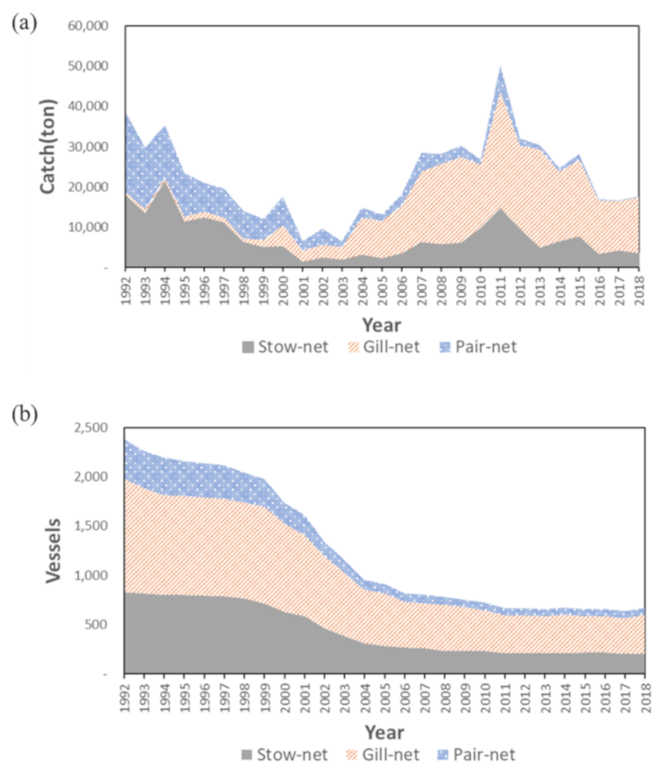
Most of the small yellow croakers were caught by using stow-nets and pair-trawls before 2000; however, after 2000, the small yellow croakers have been mostly caught by using gill-nets (Figure 1a). This is largely due to changes in fishing grounds and fishing methods across different fisheries, following the enforcement of the South Korea-China Fishery Agreement in 2001. The fishing methods and gears used in pair-trawl fisheries were changed from bottom trawls to middle and surface trawls in the mid-1990s, and the major target species changed from small yellow croakers to Spanish mackerel, chub mackerel, and anchovies [44,45]. In addition, the mesh size used in gill-net fishing has been continuously decreasing since the 1960s, and the catch capacity rapidly increased after the 2000s as the mesh size was reduced to 51 mm [46]. Consequently, the most common type of fishery for small yellow croakers changed from pair-trawl to gill-net fisheries.
The number of vessels associated with the various fisheries has continuously decreased since 1992 due to a vessel buyback program and other initiatives (Figure 1b). In 2018, the number of vessels associated with gill-nets was the highest (395), followed by stow-nets (207), and pair-trawls (70). Furthermore, the engine power (EP) of fishing vessels based on the fishing type has considerably increased from 196 EP in 1992 to 709 EP in 2018 for gill-net fisheries, 355 EP to 820 EP for stow-net fisheries, and 567 EP to 1340 EP for pair-trawl fisheries.
The profit per vessel of stow-net fishery recorded at the lowest in 1998 and has increased until 2018 (Figure 2). Similar to the stow-net fishery, the profit per vessel of gill-net fishery has been increased until 2018 since it recorded the lowest in 1993. However, the profit per vessel of pair-trawl has changed quite extremely since the major change in their target species.
2.2. Generalized Linear Model for CPUE Standardization
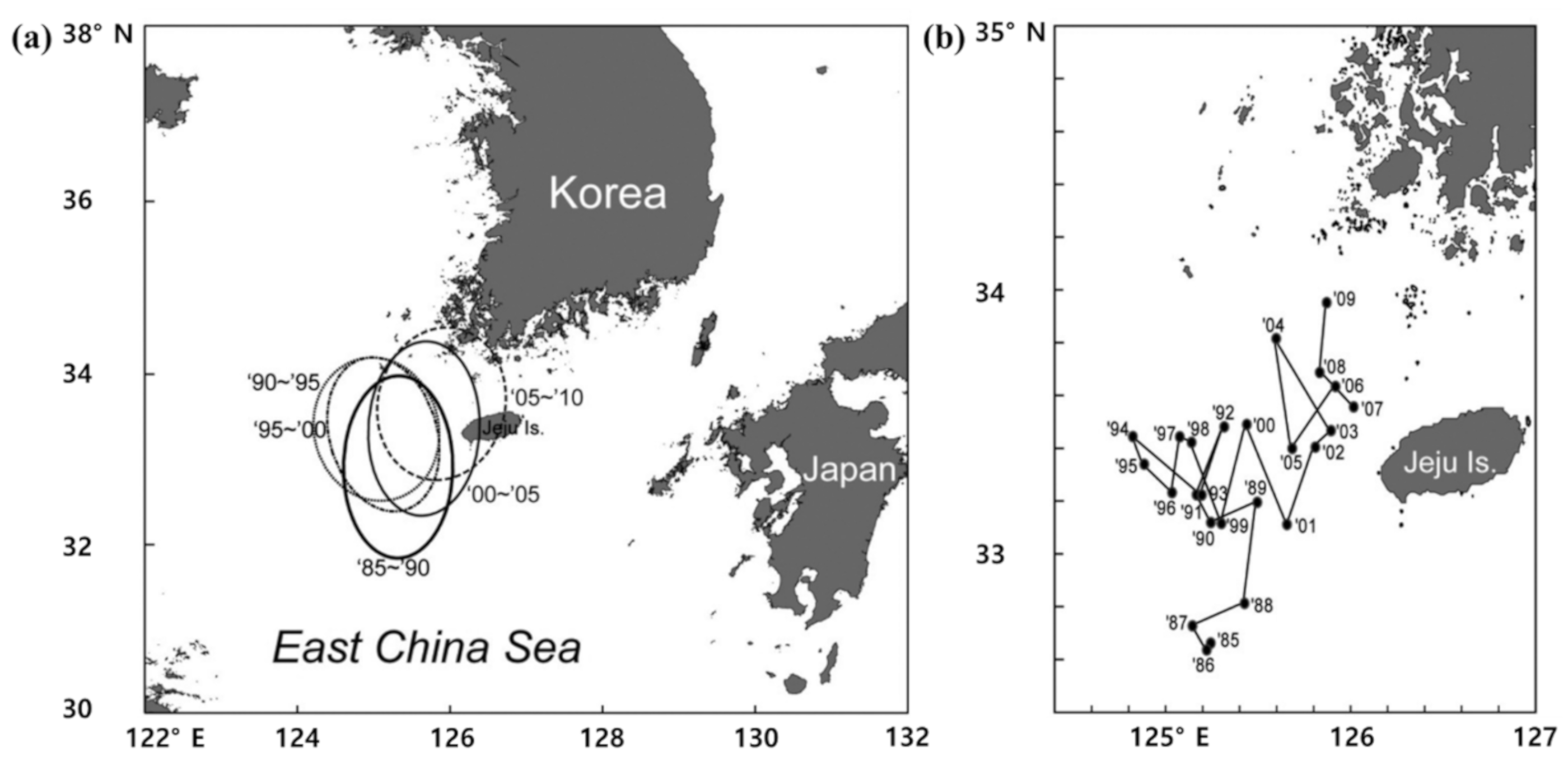
The GLM method proposed by Gavaris [43] has been extensively used to standardize the fishing capacities of different fisheries for the stock assessments of a single fish species [41,47,48]. The GLM is used to calculate a standardized catch per unit effort (CPUE) using the explanatory variables that influence the CPUE and can account for different fishing capacities across years and fishing method [41]. Previous studies have also used the year and fishing type as the explanatory variables in this model [15]. Lim et al. [49] identified fishing ground as another major variable because the major fishing grounds of small yellow croakers have continuously shifted northeast (Figure 3).
Therefore, we selected and analyzed the year, fishing type, and shift in fishing grounds as the explanatory variables in our GLM, which could influence the CPUE of the small yellow croaker, as represented in Equation (1):
where denotes the CPUE and denotes the reference CPUE for each explanatory variable, namely the year, fishing type, and shift in fishing grounds. denotes the explanatory variable, and denotes the classification criterion in the explanatory variable. denotes the relative fishing capacity of j in the explanatory variable . Finally, denotes a dummy variable, which is set to 1 if the data fall under the category, and to 0, if otherwise. denotes a normal distribution where the mean is 0, and the variance is . When Equation (1) is rearranged by applying log on both sides, Equation (2) is obtained:
When Equation (2) is modified for CPUE standardization based on the fishery type for small yellow croakers, Equation (3) is obtained:
where denotes the difference in fishing capacity by year, for which the data from 1992 to 2018 were used. denotes the difference in fishing capacity by fishing type, including stow-net, gill-net, and pair-trawl. denotes the difference in fishing capacity at the central fishing grounds, for which 1992–1999, 2000–2004, and 2005–2018 were defined as the dummy variables. Finally, the change in fishing capacity based on the shift in the central fishing ground by fishing type was considered as an interaction variable, denoted as .
Coefficients for standardizing CPUE are inferred by linear regression following Equation (3), and then the standardized CPUE by years, fishing types, and main fishing grounds can be calculated. Standardized efforts can be calculated by catch divided by standardized CPUE of each fishing type. By adding standardized efforts of each fishing type, the total standardized catch efforts for the fisheries’ stock assessment can be calculated.
2.3. Surplus Production Model
The surplus production model (SPM) can be used to assess fish stocks based on catch and fishing effort time series data. The SPM has been extensively used for the assessment of stocks of various fish species because it can perform stock assessments even with insufficient data [17,19,27,50,51,52]. The SPM expresses the current biomass based on the relationship between past biomass and the growth and catch of the corresponding stock, as follows:
where denotes the biomass of a year y, denotes the stock growth, and denotes the catch of the year y. Furthermore, based on the assumption, the SPM can be expressed using Equations (5) and (6).
where denotes the intrinsic growth rate of the fish stocks, and K denotes the carrying capacity. Equation (5) was proposed as a logistic growth function by Schaefer [39], and Equation (6) as an exponential growth function by Fox [40].
In the estimation based on the SPM, the relationship between the catchability coefficient (q) and biomass is generally assumed to be constant [53]. In other words, the CPUE can be obtained by dividing the catch by the fishing effort and the relationship between the catchability coefficient (q) and biomass can be expressed using Equation (7).
2.4. Bayesian State-Space Model
To estimate the biomass of Korean small yellow croakers using the SPM, we used the Bayesian state-space model suggested by Meyer and Millar [22]. The biomass was reparameterized into a biomass-to-K ratio () for speed mixing. Consequently, the surplus production function can be expressed using Equations (8) and (9):
Equation (8) was obtained by substituting Equation (5), which is the function of Schaefer (1954), in Equation (4), and Equation (9) was obtained by substituting Equation (6), which is the function of Fox (1970), in Equation (4). Furthermore, Equation (7), which is a function for the observation data, can be reformulated into Equation (10):
The Bayesian state-space model can infer the posterior distribution of each parameter by combining prior distribution established from prior information and the likelihood derived from the observation data, according to the Bayes’ theorem [54,55]. Furthermore, the parameters of interest required for fish stock assessment can be estimated based on the derived posterior distribution. The joint prior density for the parameters of interest can be expressed as Equation (11):
Regarding prior distributions, informative prior distribution was assumed for internal growth (r) and environmental capacity (K), and non-informative prior distribution was assumed for fishing efficiency coefficient (q), according to Millar and Meyer [18]. To set informative prior distributions, we referred to Sim and Nam [15].
In addition, sensitivity analysis was performed for the initial values per the suggestion of Punt and Hilborn [36]. Typically, the r value for fish stocks is predicted to lie within the range of 0.015–1.5 [56]. However, K has a relatively broad range. Therefore, we assumed the r value to be 0.5 for sensitivity analysis and a non-informative condition for K. To assume a non-informative condition for K, the prior distributions of K were assumed to be uniform and to have inverse-gamma distributions [22,35,36]. Table 1 summarizes the prior distribution set for the estimation of Korean small yellow croaker stocks using the Bayesian state-space model.
Based on the prior distributions, the likelihood of each parameter of interest can be derived using observation data with Equation (12):
According to the Bayes’ theorem, the joint posterior distribution of each parameter of interest can be estimated by combining Equations (11) and (12) as follows:
WinBUGS (v1.4.3) program, by the Medical Research Council Biostatistics Unit, Institute of Public Health, Cambridge, the United Kingdom, used in the present study employs the Markov chain Monte Carlo (MCMC) simulation to derive the joint posterior distributions. The MCMC simulation involves a probabilistic estimation of posterior distributions through random sampling and replaces the multidimensional integral calculation required for deriving the parameter of interest with statistical extractions [53,54]. However, as it is challenging to generate a random sample from the joint probability distribution of multidimensional variables, the variables are sequentially extracted from conditional probability distributions of other variables using Gibbs sampling. Various algorithms are used to estimate the posterior distribution in MCMC simulations by using Gibbs sampling. WinBUGS program derives the posterior distribution by selecting an appropriate algorithm according to the distribution of each parameter of interest [57,58,59,60].
By performing the above process m times, the posterior distribution for each parameter of interest can be estimated using Equation (15):
Model Implementation and Comparison
Six scenarios were set up and analyzed by applying the assumptions of three prior distributions for the Schaefer and Fox functions. A total of 300,000 samples were collected and used to obtain estimates based on the Bayesian state-space model. Among them, the initial 50,000 samples that were not consistent with the posterior distribution were discarded by setting the burn-in period. Furthermore, the twenty fifth sample was extracted to minimize sample correlation that was observed during the extraction process. Finally, the posterior distribution was derived using 10,000 samples.
For comparing model fitness by scenario, we applied the deviance information criterion (DIC), which is useful in the comparison of models using Bayesian reasoning, as shown in Equation (16). The DIC can consider the fitness of the model (model complexity) and that of the analysis results simultaneously [61,62].
where denotes the likelihood of the estimated parameter, denotes the deviation, and denotes the posterior mean deviation. In particular, and are used to evaluate the fitness of the model and that of the analysis results, respectively.
3. Results
3.1. GLM Analysis Results and Model Comparison
The GLM results from 2000 to 2018 are shown in Table A1. The differences in fishing capacity based on the fishing type and shifts in fishing grounds were significant (P < 0.001). When the small yellow croaker stocks were analyzed using the Bayesian state-space model with the standardized CPUE, the Monte Carlo error for the parameters in all scenarios was lower than 5% of the standard error, this indicates convergence of the model [62]. In addition, as illustrated in Figure 4, the shapes of the posterior distributions estimated were not similar to those of the prior distributions in each scenario. Consequently, the data were considered to have sufficient information for model estimation [63]. Most graphs were skewed right, and therefore, the medians were used as the representative values.
The estimates of the model for each scenario have been outlined in Table 2. First, when the Schaefer function was used, the difference between the DICs based on the variation in the prior distributions was lower than two, which indicated no significant difference. In contrast, the Fox function was more suitable when the non-informative prior distribution was assumed than when the informative prior distribution was assumed, as there was a significant difference.
In comparing the two functions, regardless of the prior distribution assumption, the assumption of the Fox function was more suitable than that of the Schaefer function in all scenarios. Therefore, the most suitable analytical model was the Fox model with an inverse-gamma distribution for the K value. In addition, the R2 value of the estimate was very high, at 0.99. As illustrated in Figure 5, all standardized CPUEs were included in the posterior 95% confidence level of the CPUE estimated using the Bayesian state-space model. Therefore, small yellow croaker stocks were assessed based on the estimates of the Bayesian state-space model, with an inverse-gamma distribution, using the Fox model, which has the lowest DIC.
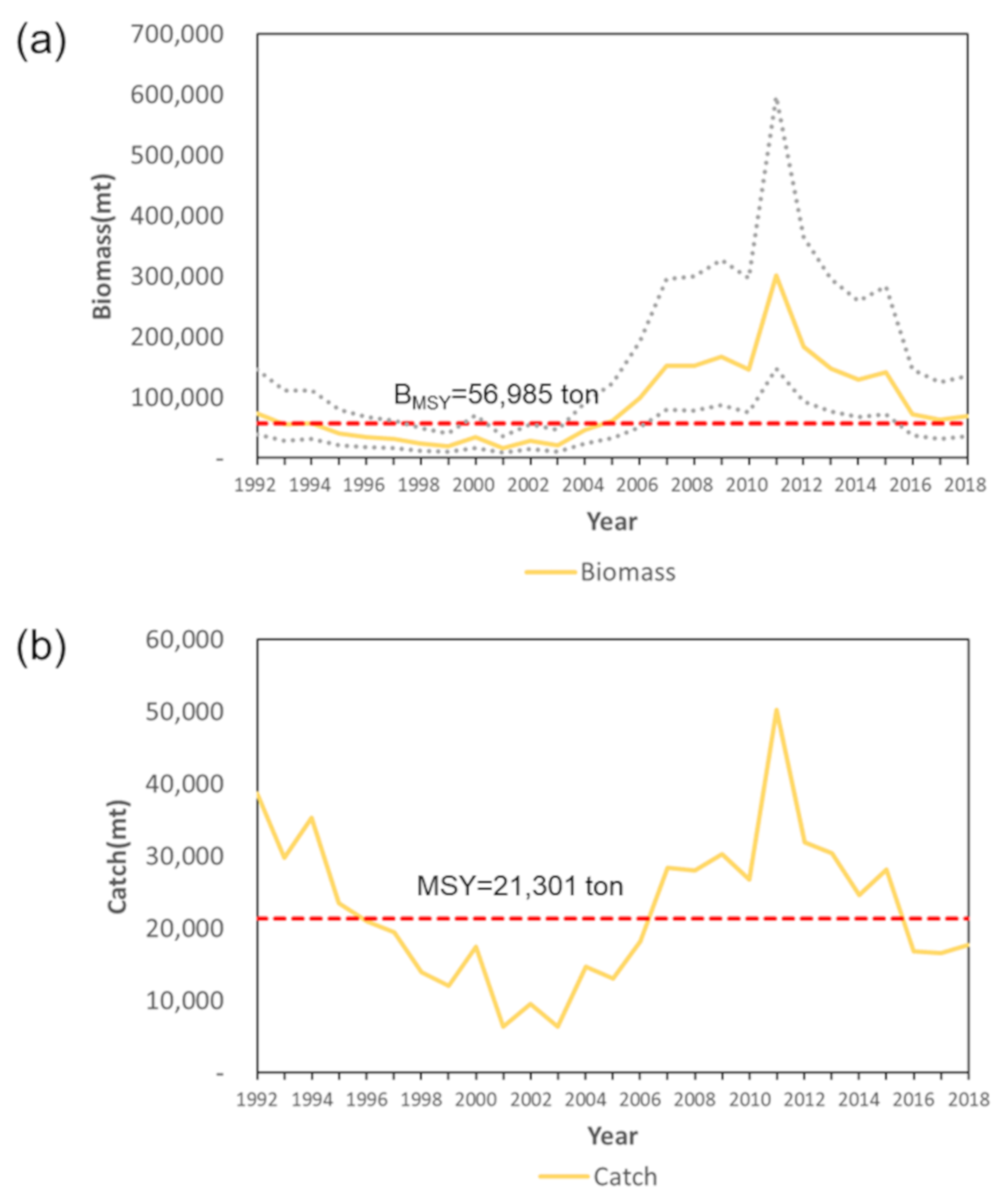
According to the small yellow croaker stock assessments, as illustrated in Figure 6, the fish biomass has decreased since 1992 and reached its lowest level of 16,800 tons in 2001. Subsequently, the fish stocks increased gradually, and the highest value was recorded in 2011; thereafter, it decreased again. The fish biomass was 69,150 tons in 2018, or 121% of the biomass at sustainable yield (BMSY) (56,985 tons). However, since 1992, its biomass has exhibited considerable variations, and it had dropped below the BMSY between 1993 and 2004.
Since 2011, the biomass and catch of small yellow croakers have decreased continuously. Small yellow croaker catch has also continuously decreased since 1992, and the lowest value of 6380 tons was recorded in 2001. Since then, the catch has gradually recovered with an increase in biomass, and its highest value of 59,226 tons was recorded in 2011. Subsequently, the catch decreased again, and it was only 17,683 tons in 2018. Comparing it with the profits of gill-net and stow-net fisheries (Figure 2), it seems reasonable that they got relatively low profits in the 1990s when the biomass level of small yellow croaker in most years was lower than BMSY.
3.2. Analysis of Appropriate TAC Levels
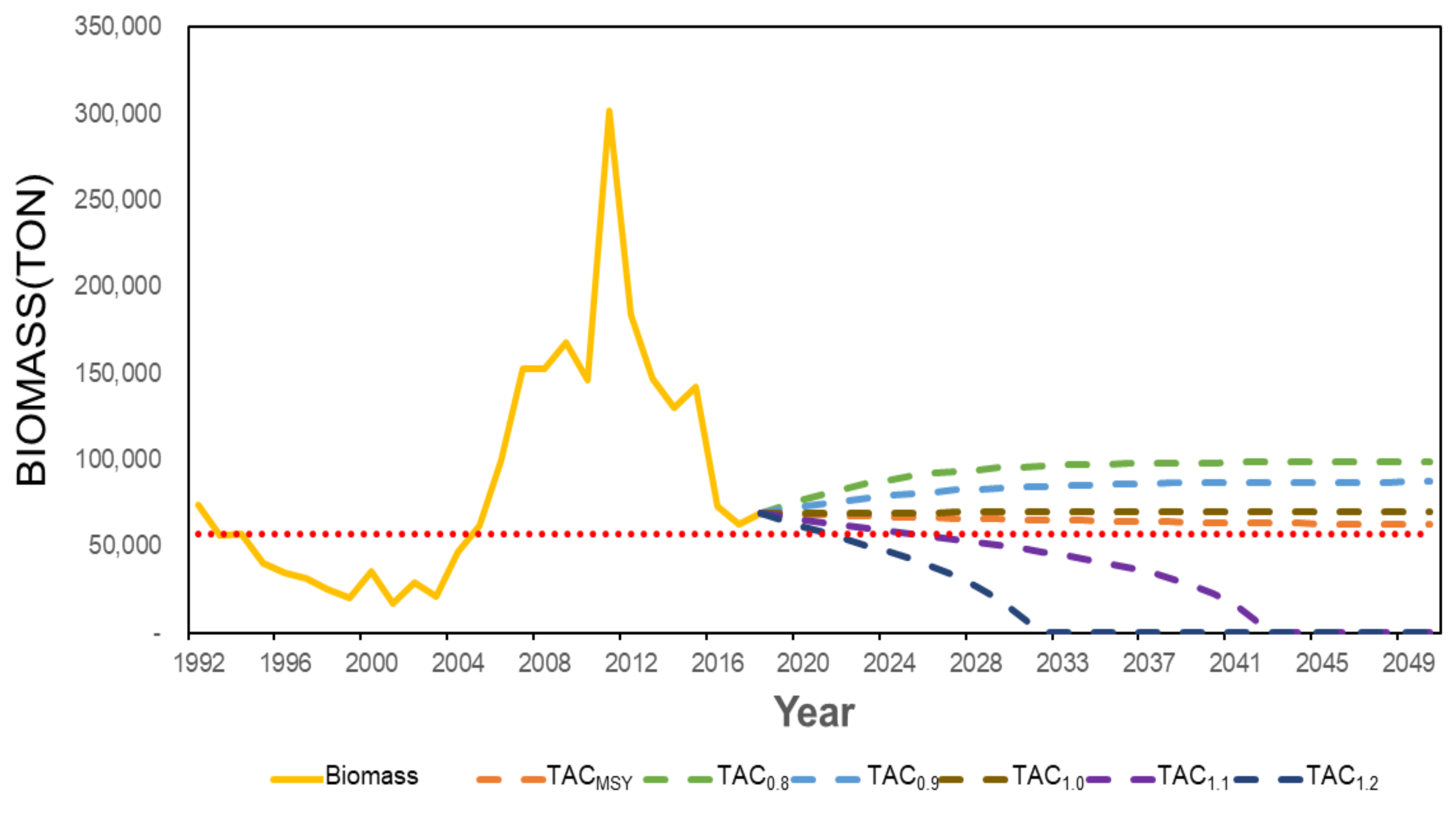
To analyze the appropriate TAC levels that would facilitate the effective management and recovery of small yellow croaker stocks in the future, scenario analysis was performed based on the stock assessment results. Specifically, future biomass variations were estimated for each scenario under the following annual TAC level settings: a 20% increase (TAC1.2), 10% increase (TAC1.1), 10% decrease (TAC0.9), 20% decrease (TAC0.8), and 20,800 tons (TAC1.0), which was the mean catch of small yellow croakers by gill-net, stow-net, and pair-trawl fisheries in 2014–2018, and the MSY (TACMSY) of 21,301 tons.
According to the analysis results, as shown in Figure 7, a 10% increase from the current level of catch could decrease the future biomass of small yellow croakers. However, when the TAC level was set to the current MSY level, their biomass was relatively stable.
4. Discussion
The results of the small yellow croaker stock assessments using the Bayesian state-space model revealed that it is necessary to manage the biomass of the small yellow croaker to ensure stable catch in the future. In particular, the estimates of future small yellow croaker biomass under different TAC scenarios suggested that their biomass would decrease with even a 10% increase in catch when compared with the current catch levels. Therefore, to prevent the reduction in small yellow croaker catch, as in the past, efforts should be made to maintain the small yellow croaker biomass at the current or MSY levels.
According to the sensitivity analysis results obtained using the Bayesian state-space model, the adoption of a non-informative prior distribution yielded results similar to or better than those observed with the prior information distribution. In other words, even if prior information on the stocks is insufficient, it is not necessary to discard the Bayesian state-space analysis, as demonstrated by Thorson and Cope [37]. Particularly, the estimates based on the Fox function demonstrated that the assumption of non-informative prior distribution could yield superior results when compared with the estimates under the assumption of informative prior distribution. Consequently, even if prior information exists for stock assessment activities based on the Bayesian state-space model in the future, performing an additional sensitivity analysis using non-informative prior information could facilitate more reliable stock assessment results.
Furthermore, in the sensitivity analysis, the DIC difference due to the change in growth function was greater than that due to the change in prior distribution. Specifically, the largest DIC difference based on prior distribution was 3.712 in the Fox model. However, the DIC difference based on the Schaefer and Fox function was 11.727. Therefore, a change in growth function could have a greater influence on the reliability of the estimates of the Bayesian state-space model than a change in prior distribution. Notably, when the Schaefer function was applied, the small yellow croaker biomass of 2018 was estimated at 85% of the BMSY, which was substantially different from the results obtained with the Fox function, where the biomass was greater than the BMSY. The sensitivity analysis for the Bayesian state-space model estimates to date has focused on prior distributions. However, in future Bayesian state-space model estimates, more reliable stock assessments could be obtained if growth function analyses are performed in addition to sensitivity analysis for prior distributions.
In the present study, the Pella–Tomlinson [64] function, which has been extensively used in fish stock assessments in addition to the Schaefer and Fox functions, could not be applied. This is because in the estimation with the Bayesian state-space model, the estimates of the Pella–Tomlinson function under an assumption of a similar prior distribution were not consistent with the parameter of interest. It could be more challenging for the Pella–Tomlinson function to achieve convergence with the model because variables are added based on parameter p in the analysis with the growth function model. However, more reliable results could be obtained in the future if the Pella–Tomlinson function can also be considered. Furthermore, other approaches should be adopted, such as model analyses based on age-structure models. In addition, there has been an increasing impact of climate change on fisheries’ resources. However, in this study, only a “shift in fishing grounds” was considered as an environmental factor. In considering other variables, such as sea surface temperature, more reliable results could surface [65,66]. Therefore, there is a need for future studies to explore this variable, among others. Finally, we could not consider maximum economic yield (MEY) and ITQ, which is another catch regulation due to the lack of available economic data. If these are considered with the appropriate data, a more effective management plan for the small yellow croaker could be derived.
Author Contributions
Conceptualization, M.-J.C. and D.-H.K.; methodology, M.-J.C. and D.-H.K.; software, M.-J.C.; validation, M.-J.C. and D.-H.K.; formal analysis, M.-J.C.; investigation, D.-H.K.; resources, M.-J.C. and D.-H.K.; data curation, M.-J.C. and D.-H.K.; writing—original draft preparation, M.-J.C. and D.-H.K.; writing—review and editing, D.-H.K.; visualization, M.-J.C.; supervision, D.-H.K.; project administration, D.-H.K.; funding acquisition, D.-H.K. All authors have read and agreed to the published version of the manuscript.
Funding
This research received no external funding.
Conflicts of Interest
The authors declare no conflict of interest.
Appendix A

Table A1.
Significance level of the generalized linear model.
| Variable | Coefficient | Std. Error | t-Statistics | p-Value |
|---|---|---|---|---|
| (Intercept) | 0.294 | 0.316 | 0.931 | 0.357 |
| year1993 | −0.042 | 0.4 | −0.106 | 0.916 |
| year1994 | 0.072 | 0.4 | 0.179 | 0.858 |
| year1995 | −0.069 | 0.4 | −0.172 | 0.865 |
| year1996 | −0.153 | 0.4 | −0.383 | 0.703 |
| year1997 | −0.208 | 0.4 | −0.52 | 0.605 |
| year1998 | −0.444 | 0.4 | −1.112 | 0.272 |
| year1999 | −0.377 | 0.4 | −0.944 | 0.350 |
| year2000 | 1.818 | 0.46 | 3.952 | 0.000 *** |
| year2001 | 0.836 | 0.46 | 1.817 | 0.076 . |
| year2002 | 1.496 | 0.46 | 3.252 | 0.002 ** |
| year2003 | 1.17 | 0.46 | 2.543 | 0.014 * |
| year2004 | 2.145 | 0.46 | 4.663 | 0.000 *** |
| year2005 | 2.724 | 0.437 | 6.231 | 0.000 *** |
| year2006 | 3.272 | 0.437 | 7.484 | 0.000 *** |
| year2007 | 3.769 | 0.437 | 8.619 | 0.000 *** |
| year2008 | 3.631 | 0.437 | 8.305 | 0.000 *** |
| year2009 | 3.761 | 0.437 | 8.603 | 0.000 *** |
| year2010 | 3.549 | 0.437 | 8.118 | 0.000 *** |
| year2011 | 4.547 | 0.437 | 10.399 | 0.000 *** |
| year2012 | 3.855 | 0.437 | 8.818 | 0.000 *** |
| year2013 | 3.516 | 0.437 | 8.043 | 0.000 *** |
| year2014 | 3.448 | 0.437 | 7.886 | 0.000 *** |
| year2015 | 3.658 | 0.437 | 8.367 | 0.000 *** |
| year2016 | 2.76 | 0.437 | 6.312 | 0.000 *** |
| year2017 | 2.638 | 0.437 | 6.034 | 0.000 *** |
| year2018 | 2.752 | 0.437 | 6.294 | 0.000 *** |
| pair_trawl | 3.189 | 0.245 | 13.029 | <2e−16 *** |
| stow_net | 2.509 | 0.245 | 10.249 | 0.000 *** |
| pair_trawl:move23 | −2.023 | 0.395 | −5.124 | 0.000 *** |
| stow_net:move23 | −2.601 | 0.395 | −6.59 | 0.000 *** |
| pair_trawl:move24 | −4.065 | 0.307 | −13.248 | <2e−16 *** |
| stow_net:move24 | −3.042 | 0.307 | −9.912 | 0.000 *** |
Significance level: *** p ≤ 0.0001; ** p ≤ 0.001; * p ≤ 0.01; ‘.’ p ≤ 0.05.
References
- Lee, S.G.; Midani, A.R. National comprehensive approaches for rebuilding fisheries in South Korea. Mar. Policy 2014, 45, 156–162. [Google Scholar] [CrossRef]
- National Institute of Fisheries Science. Fishes of the Pacific Ocean; National Institute of Fisheries Science: Busan, Korea, 2015.
- Park, J.M. Historical consideration of Production and using of a croaker. Korean J. Agric. Hist. 2010, 9, 197–222. [Google Scholar]
- Choi, M.J.; Kim, D.H. Comparing surplus production models for selecting effective stock assessment model: Analyzing potential yield of East Sea, Republic of Korea. Ocean Polar Res. 2019, 41, 183–191. [Google Scholar]
- Choi, M.J.; Kim, D.H.; Choi, J.H. Comparative analysis of stock assessment models for analyzing potential yield of fishery resources in the West Sea, Korea. J. Korean Soc. Fish. Ocean Technol. 2019, 55, 206–216. [Google Scholar] [CrossRef]
- Korean Statistical Information Service. Available online: http://kosis.kr/ (accessed on 18 January 2020).
- National Institute of Fisheries Science. Target Fish Species of Fisheries Resources Recovery Project. Available online: https://www.nifs.go.kr/page?id=rec_fish (accessed on 5 February 2020).
- Kim, D.H. Evaluating the TAC policy in the sandfish stock rebuilding plan. J. Fish. Bus. Adm. 2015, 46, 29–39. [Google Scholar] [CrossRef]
- Kim, D.Y.; Lee, J.S.; Kim, D.H. A study on establishing the performance evaluation system of the fish stock rebuilding plans. J. Fish. Bus. Adm. 2011, 42, 15–29. [Google Scholar]
- National Law Information Center. Enforcement Decree of the Fisheries Resources Management Act. Available online: http://www.law.go.kr (accessed on 5 February 2020).
- Jeong, M.J.; Nam, J.O. Effectiveness analysis on comb pen shell based on TAC system. J. Fish. Bus. Adm. 2016, 47, 15–33. [Google Scholar] [CrossRef] [Green Version]
- Sim, S.H.; Lee, J.S.; Oh, S.Y. An analysis of the effects in the TAC system by analyzing catch of TAC target species. Ocean Polar Res. 2020, 42, 157–169. [Google Scholar]
- Korea Fisheries Resources Agency. TAC Introduction. Available online: https://www.fira.or.kr/fira/fira_030601.jsp (accessed on 5 February 2020).
- National Institute of Fisheries Science. Resource Status and Restoration Recommendation of Fisheries Resources in 2017; National Institute of Fisheries Science: Busan, Korea, 2017.
- Sim, S.H.; Nam, J.O. A Stock Assessment of yellow croaker using bioeconomic model: A case of single species and multiple fisheries. Ocean Polar Res. 2015, 37, 161–177. [Google Scholar] [CrossRef]
- Zhang, C.I.; Kim, S.; Yoon, S.B. Stock assessment and management implications of small yellow croaker in Korean waters. Korean J. Fish. Aquat. Sci. 1992, 25, 282–290. [Google Scholar]
- Clarke, R.P.; Yoshimoto, S.S.; Pooley, S.G. A bioeconomic analysis of the Northwestern Hawaiian Islands lobster fishery. Mar. Resour. Econ. 1992, 7, 115–140. [Google Scholar] [CrossRef]
- Millar, R.B.; Meyer, R. Non-linear state space modelling of fisheries biomass dynamics by using Metropolis-Hastings within-Gibbs sampling. J. R. Stat. Soc. C Appl. 2000, 49, 327–342. [Google Scholar] [CrossRef]
- Polacheck, T.; Hilborn, R.; Punt, A.E. Fitting surplus production models: Comparing methods and measuring uncertainty. Can. J. Fish. Aquat. Sci. 1993, 50, 2597–2607. [Google Scholar] [CrossRef]
- Bolker, B. Ecological Models and Data in R; Princeton University Press: Princeton, NJ, USA, 2008; pp. 233–242. [Google Scholar]
- Chaloupka, M.; Balazs, G. Using Bayesian state-space modelling to assess the recovery and harvest potential of the Hawaiian green sea turtle stock. Ecol. Model. 2007, 205, 93–109. [Google Scholar] [CrossRef]
- Meyer, R.; Millar, R.B. BUGS in Bayesian stock assessments. Can. J. Fish. Aquat. Sci. 1999, 56, 1078–1087. [Google Scholar] [CrossRef]
- Choi, M.J.; Kim, D.H.; Lee, H.W.; Seo, Y.I.; Lee, S.I. Assessing stock biomass and analyzing management effects regarding the black scraper (Thamnaconus modestus) using Bayesian state-space model. Ocean Polar Res. 2020, 42, 63–76. [Google Scholar]
- McAllister, M.K.; Pikitch, E.K.; Punt, A.E.; Hilborn, R. A Bayesian approach to stock assessment and harvest decisions using the sampling/importance resampling algorithm. Can. J. Fish. Aquat. Sci. 1994, 51, 2673–2687. [Google Scholar] [CrossRef]
- Otsuyama, K.; Kitakado, T. Bayesian state-space production models for the Indian Ocean bigeye tuna (Thunnus Obesus) and their predictive evaluation. IOTC 2016, WPTT18-19. [Google Scholar]
- Parker, D.; Winker, H.; da Silva, C.; Kerwath, S. Bayesian state-space surplus production model JABBA assessment of Indian Ocean black marlin (Makaira indica) stock. IOTC 2018, WPB16-15. [Google Scholar]
- Winker, H.; Carvalho, F.; Kapur, M. JABBA: Just another Bayesian biomass assessment. Fish. Res. 2018, 204, 275–288. [Google Scholar] [CrossRef]
- McAllister, M.K.; Pikitch, E.K.; Babcock, E.A. Using demographic methods to construct Bayesian priors for the intrinsic rate of increase in the Schaefer model and implications for stock rebuilding. Can. J. Fish. Aquat. Sci. 2001, 58, 1871–1890. [Google Scholar] [CrossRef]
- Millar, R.B. Reference priors for Bayesian fisheries models. Can. J. Fish. Aquat. Sci. 2002, 59, 1492–1502. [Google Scholar] [CrossRef]
- Van Dongen, S. Prior specification in Bayesian statistics: Three cautionary tales. J. Theor. Biol. 2006, 242, 90–100. [Google Scholar] [CrossRef] [PubMed]
- Dick, E.J.; MacCall, A.D. Depletion-based stock reduction analysis: A catch-based method for determining sustainable yields for data-poor fish stocks. Fish. Res. 2011, 110, 331–341. [Google Scholar] [CrossRef]
- Dowling, N.A.; Smith, D.C.; Knuckey, I.; Smith, A.D.; Domaschenz, P.; Patterson, H.M.; Whitelaw, W. Developing harvest strategies for low-value and data-poor fisheries: Case studies from three Australian fisheries. Fish. Res. 2008, 94, 380–390. [Google Scholar] [CrossRef]
- Free, C.M.; Jensen, O.P.; Wiedenmann, J.; Deroba, J.J. The refined ORCS approach: A catch-based method for estimating stock status and catch limits for data-poor fish stocks. Fish. Res. 2017, 193, 60–70. [Google Scholar] [CrossRef]
- Zhou, S.; Punt, A.E.; Ye, Y.; Ellis, N.; Dichmont, C.M.; Haddon, M.; Smith, D.C.; Smith, A.D. Estimating stock depletion level from patterns of catch history. Fish 2017, 18, 742–751. [Google Scholar] [CrossRef] [Green Version]
- Gelman, A. Prior distributions for variance parameters in hierarchical models. Bayesian Anal. 2006, 1, 515–534. [Google Scholar] [CrossRef]
- Punt, A.E.; Hilborn, R. Fisheries stock assessment and decision analysis: The Bayesian approach. Rev. Fish Biol. Fish. 1997, 7, 35–63. [Google Scholar] [CrossRef] [Green Version]
- Thorson, J.T.; Cope, J.M. Uniform, uninformed or misinformed? The lingering challenge of minimally informative priors in data-limited Bayesian stock assessments. Fish. Res. 2017, 194, 164–172. [Google Scholar] [CrossRef]
- Maunder, M.N. Is it time to discard the Schaefer model from the stock assessment scientist’s toolbox? Fish. Res. 2003, 1, 145–149. [Google Scholar] [CrossRef]
- Schaefer, M.B. Some aspects of the dynamics of populations important to the management of the commercial marine fisheries. IATTC Bull. 1954, 1, 23–56. [Google Scholar]
- Fox Jr, W.W. An exponential surplus-yield model for optimizing exploited fish populations. T. Am. Fish. Soc. 1970, 99, 80–88. [Google Scholar] [CrossRef]
- Hinton, M.G.; Maunder, M.N. Methods for standardizing CPUE and how to select among them. Collect Vol. Sci. Pap. ICCAT 2004, 56, 169–177. [Google Scholar]
- Kimura, D.K. Standardized measures of relative abundance based on modelling log (CPUE), and their application to Pacific Ocean perch (Sebastes alutus). ICES J. Mar. Sci. 1981, 39, 211–218. [Google Scholar] [CrossRef]
- Gavaris, S. Use of a multiplicative model to estimate catch rate and effort from commercial data. Can. J. Fish. Aquat. Sci. 1980, 37, 2272–2275. [Google Scholar] [CrossRef]
- Kim, D.Y.; Kim, B.H. Restructuring of the off-shore otter trawl fishery in Korea. J. Fish. Mar. Sci. Edu. 2004, 16, 124–141. [Google Scholar]
- Lee, D.W.; Choi, K.H.; Kang, S. Changes of fishing ground of the large pair trawl fishery off Korean Waters. Korean J. Fish. Aquat. Sci. 2013, 46, 917–922. [Google Scholar]
- Seo, Y.I.; Oh, T.Y.; Cha, H.K.; Kim, B.Y.; Jo, H.S.; Jeong, T.Y.; Lee, Y.W. Change of relative fishing power index from technological development in the small yellow croaker drift gillnet fishery. J. Korean Soc. Fish. Ocean Technol. 2019, 55, 198–205. [Google Scholar] [CrossRef]
- Nishida, T.; Bigelow, K.; Mohri, M.; Marsac, F. Comparative study on Japanese tuna longline CPUE standardization of yellowfin tuna (Thunnus albacares) in the Indian Ocean based on two methods: General linear model (GLM) and habitat-based model (HBM)/GLM combined. IOTC Proc. 2003, 6, 48–69. [Google Scholar]
- Shono, H. Application of the Tweedie distribution to zero-catch data in CPUE analysis. Fish. Res. 2008, 93, 154–162. [Google Scholar] [CrossRef] [Green Version]
- Lim, Y.N.; Kim, H.Y.; Kim, D.H. Predicting changes in fishing conditions for the small yellow croaker Larimichthys polyactis based on expansions of the Yellow Sea bottom cold water. Korean J. Fish. Aquat. Sci. 2014, 47, 419–423. [Google Scholar]
- Best, J.K.; Punt, A.E. Parameterizations for Bayesian state-space surplus production models. Fish. Res. 2020, 222, 105411. [Google Scholar] [CrossRef]
- Coppola, G.; Pascoe, S. A surplus production model with a nonlinear catch-effort relationship. Mar. Resour. Econ. 1998, 13, 37–50. [Google Scholar] [CrossRef]
- Karim, E.; Qun, L.; Hasan, S.J.; Ali, M.Z.; Hoq, M.E.; Mahmud, M.Y. Maximum sustainable yield estimates of marine captured shrimp fishery of the Bay of Bengal, Bangladesh by using surplus production model. Thalassas 2020, 36, 471–480. [Google Scholar] [CrossRef]
- Haddon, M. Modelling and Quantitative Methods in Fisheries; CRC Press: New York, NY, USA, 2010; pp. 285–333. [Google Scholar]
- Kim, D.H. Bayesian Statistics Using R and WinBUGS; Freedom Academy: Paju, Korea, 2013; pp. 87–248. [Google Scholar]
- Ntzoufras, I. Bayesian Modeling Using WinBUGS; John Wiley & Sons: Hoboken, NJ, USA, 2011; Volume 698, p. 520. [Google Scholar]
- Martell, S.; Froese, R. A simple method for estimating MSY from catch and resilience. Fish 2013, 14, 504–514. [Google Scholar] [CrossRef]
- Gilks, W.R.; Wild, P. Adaptive rejection sampling for Gibbs sampling. J. R. Stat. Soc. C Appl. 1992, 41, 337–348. [Google Scholar] [CrossRef]
- Kéry, M.; Schaub, M. Bayesian Population Analysis using WinBUGS: A Hierarchical Perspective; Academic Press: Cambridge, UK, 2011; p. 55. [Google Scholar]
- Lunn, D.J.; Thomas, A.; Best, N.; Spiegelhalter, D. WinBUGS-a Bayesian modelling framework: Concepts, structure, and extensibility. Stat. Comput. 2000, 10, 325–337. [Google Scholar] [CrossRef]
- Neal, R.M. Markov Chain Monte Carlo Methods Based on ‘Slicing’ the Density Function. 1997, pp. 1–27. Available online: http://citeseerx.ist.psu.edu/viewdoc/download?doi=10.1.1.48.886&rep=rep1&type=pdf (accessed on 17 February 2020).
- Spiegelhalter, D.J.; Best, N.G.; Carlin, B.P.; Van Der Linde, A. Bayesian measures of model complexity and fit. J. R. Stat. Soc. B 2002, 64, 583–639. [Google Scholar] [CrossRef] [Green Version]
- Spiegelhalter, D.J.; Thomas, A.; Best, N.; Lunn, D. WinBUGS User Manual. 2003, pp. 1–60. Available online: https://www.mrc-bsu.cam.ac.uk/wp-content/uploads/manual14.pdf (accessed on 15 March 2020).
- Punt, A.E.; Hilborn, R. Bayesian Stock Assessment Methods in Fisheries: User’s Manual; Food and Agriculture Organization: Rome, Italy, 2001; pp. 1–68. [Google Scholar]
- Pella, J.J.; Tomlinson, P.K. A generalized stock production model. IATTC Bull. 1969, 13, 416–497. [Google Scholar]
- Chen, Y.; Shan, X.; Wang, N.; Jin, X.; Guan, L.; Gorfine, H.; Yang, T.; Dai, F. Assessment of fish vulnerability to climate change in the Yellow Sea and Bohai Sea. Mar. Freshw. Res. 2020, 71, 729–736. [Google Scholar] [CrossRef]
- Shan, X.; Li, X.; Yang, T.; Sharifuzzaman, S.M.; Zhang, G.; Jin, X.; Dai, F. Biological responses of small yellow croaker (Larimichthys polyactis) to multiple stressors: A case study in the Yellow Sea, China. Acta Oceanol. Sin. 2017, 36, 39–47. [Google Scholar] [CrossRef]
Figure 1.
Small yellow croaker catch by fishing type (a) and number of vessels (b) from 1992 to 2018.
Figure 1.
Small yellow croaker catch by fishing type (a) and number of vessels (b) from 1992 to 2018.

Figure 2.
Profit by fishing type from 1992 to 2019.

Figure 3.
Fishery ground ellipses computed using the catch per unit effort distribution of small yellow croakers in the three fisheries under different periods (a) and the centers of fishing grounds in different fishing years (b) [49].
Figure 3.
Fishery ground ellipses computed using the catch per unit effort distribution of small yellow croakers in the three fisheries under different periods (a) and the centers of fishing grounds in different fishing years (b) [49].

Figure 4.
Prior distributions (dashed line) and posterior distributions (solid line) of K and r assessed using the Bayesian state-space model.
Figure 4.
Prior distributions (dashed line) and posterior distributions (solid line) of K and r assessed using the Bayesian state-space model.

Figure 5.
Standardized catch per unit effort (CPUE) and the 2.5th (lower dotted line), 50th (median; red line), and 97.5th (upper dotted line) percentiles from the posterior distribution of CPUE based on the Bayesian state-space model using the Fox function as a non-informative prior distribution (inverse-gamma distribution) of the K assumption.

Figure 6.
Change in the annual stock biomass trajectories with 95% confidence intervals with biomass at sustainable yield (BMSY) (a) and catch in comparison with the maximum sustainable yield (b) of small yellow croakers based on the Bayesian state-space model.
Figure 6.
Change in the annual stock biomass trajectories with 95% confidence intervals with biomass at sustainable yield (BMSY) (a) and catch in comparison with the maximum sustainable yield (b) of small yellow croakers based on the Bayesian state-space model.

Figure 7.
Forecasting changes in small yellow croaker biomass under total allowable catch scenarios based on the Bayesian state-space model with a historical line (yellow line).
Figure 7.
Forecasting changes in small yellow croaker biomass under total allowable catch scenarios based on the Bayesian state-space model with a historical line (yellow line).

Table 1.
Summary of prior distributions used for the sensitivity analysis with the Bayesian state-space model.
Table 1.
Summary of prior distributions used for the sensitivity analysis with the Bayesian state-space model.
| Parameter | Informative Prior Distribution | Non-Informative Prior Distribution | |
|---|---|---|---|
| Uniform | Inverse-Gamma | ||
| r | Lognormal (−1.1, 0.512) | Lognormal (−0.69, 0.512) | Lognormal (−0.69, 0.512) |
| K | Inverse-lognormal (12.38, 0.752) | Uniform (10,000–100,000,000) | Inverse-gamma (0.01, 0.01) |
| q | Inverse-gamma (1,1) | Inverse-gamma (1,1) | Inverse-gamma (1,1) |
| Inverse-gamma (3.79, 0.01) | Inverse-gamma (3.79, 0.01) | Inverse-gamma (3.79, 0.01) | |
| Inverse-gamma (1.71, 0.01) | Inverse-gamma (1.71, 0.01) | Inverse-gamma (1.71, 0.01) | |
Table 2.
Results of the Bayesian state-space model under different assumptions.
| Parameter | Schaefer | Fox | ||||
|---|---|---|---|---|---|---|
| Informative K | Non-Informative K | Informative K | Non-Informative K | |||
| Lognormal K | Uniform | Inverse-Gamma | Log-Normal K | Uniform | Inverse-Gamma | |
| r | 0.4469 | 0.5426 | 0.5703 | 0.3273 | 0.3854 | 0.3738 |
| K (ton) | 214,100 | 198,700 | 187,600 | 169,700 | 148,500 | 154,900 |
| q | 2.03E-04 | 2.31E-04 | 2.46E-04 | 2.35E-04 | 2.72E-04 | 2.63E-04 |
| MSY (maximum sustainable yield) | 23,920 | 26,954 | 26,747 | 20,433 | 21,054 | 21,301 |
| B2018/BMSY | 0.85 | 0.82 | 0.82 | 1.24 | 1.22 | 1.21 |
| 1.16E-04 | 1.13E-04 | 1.10E-04 | 1.33E-04 | 1.46E-04 | 1.43E-04 | |
| 0.03117 | 0.03382 | 0.03559 | 0.01848 | 0.01402 | 0.01473 | |
| R2 | 0.96 | 0.96 | 0.95 | 0.99 | 0.99 | 0.99 |
| DIC (deviance information criterion) | 149.599 | 150.050 | 150.953 | 142.938 | 139.631 | 139.226 |
© 2020 by the authors. Licensee MDPI, Basel, Switzerland. This article is an open access article distributed under the terms and conditions of the Creative Commons Attribution (CC BY) license (http://creativecommons.org/licenses/by/4.0/).
Share and Cite
MDPI and ACS Style
Choi, M.-J.; Kim, D.-H. Assessment and Management of Small Yellow Croaker (Larimichthys polyactis) Stocks in South Korea. Sustainability 2020, 12, 8257. https://0-doi-org.brum.beds.ac.uk/10.3390/su12198257
AMA Style
Choi M-J, Kim D-H. Assessment and Management of Small Yellow Croaker (Larimichthys polyactis) Stocks in South Korea. Sustainability. 2020; 12(19):8257. https://0-doi-org.brum.beds.ac.uk/10.3390/su12198257
Chicago/Turabian StyleChoi, Min-Je, and Do-Hoon Kim. 2020. "Assessment and Management of Small Yellow Croaker (Larimichthys polyactis) Stocks in South Korea" Sustainability 12, no. 19: 8257. https://0-doi-org.brum.beds.ac.uk/10.3390/su12198257
Note that from the first issue of 2016, this journal uses article numbers instead of page numbers. See further details here.