Article

Spatiotemporal Analysis of the Nonlinear Negative Relationship between Urbanization and Habitat Quality in Metropolitan Areas

Department of Environmental Science and Engineering, Fudan University, 2005 Songhu Road, Shanghai 200438, China
*
Author to whom correspondence should be addressed.
Sustainability 2020, 12(2), 669; https://0-doi-org.brum.beds.ac.uk/10.3390/su12020669
Submission received: 24 December 2019 / Revised: 11 January 2020 / Accepted: 13 January 2020 / Published: 16 January 2020

Abstract

:
Urbanization intensity (UI) affects habitat quality (HQ) by changing land patterns, nutrient conditions, management, etc. Therefore, there is a need for studies on the relationship between UI and HQ and quantification of separate urbanization impacts on HQ. In this study, the relationship between HQ and UI and the direct and indirect impacts of urbanization on HQ were analyzed for the Yangtze River Delta Urban Agglomeration (YRDUA) from 1995 to 2010. The results indicated that the regional relationship between HQ and UI was nonlinear and negative, with inflection points where urbanization reached 20% and 80%. Furthermore, depending on different urbanization impacts, the relationship types generally changed from a steady decrease to stable in different cities. Negative indirect impacts accelerate habitat degradation, while positive impacts partially offset habitat degradation caused by land conversion. The average offset extent was approximately 28.23%, 17.41%, 22.94%, and 16.18% in 1995, 2000, 2005, and 2010, respectively. Moreover, the dependency of urbanization impacts on human demand in different urbanization stages was also demonstrated. The increasing demand for urban land has exacerbated the threat to ecological areas, but awareness about the need to protect ecological conditions began to strengthen after the antagonistic stage of urbanization.

1. Introduction

Since the 20th century, urbanization, including population shifting, urban expansion, economic development and so on, has been one of the most significant characteristics of human civilization [1,2]. The progress of urbanization has led to more human demand that needs to be provided for by the ecosystem services in natural ecosystems [3]. Grimm at al. found that the unprecedented rates of urban population growth over the past century have occurred on less than 3% of the global terrestrial surface, yet the impact has been global, with 78% of carbon emissions, 60% of residential water use, and 76% of wood used for industrial purposes attributed to urban areas [4]. At the same time, urbanization has brought significant land conversion from ecological spaces to urban usage, which creates seminatural or completely artificial ecosystems. In contrast to natural ecosystems, the main driving force of habitat patterns in these ecosystems is anthropogenic activity. Fertilization, irrigation, unified management, species introduction and other alterations are commonly seen in urban landscapes and have caused various impacts on habitats in terms of soil composition and nutrients [5], water, heat and carbon balance [6], species communities [7,8], atmospheric and climatic conditions [9], etc. In other words, the impact on natural ecosystems will affect the city itself. Therefore, quantifying the eco-environmental dynamic variation in the urbanization gradient and identifying the ecological impacts of urbanization provide an efficacious approach for decoupling human well-being from the consumption of natural capital [10].
In the context of urbanization, eco-environmental variation is spatially organized and dominates the composition and structure of habitats from the core urban area to the outskirts [11]. It has been widely believed that urbanization threatens biodiversity, with areas of high urbanization levels having impoverished species community composition [12,13,14] due to environmental stresses (e.g., poor soil quality, high pollution, and limited habitat) and the artificial conversion of ecological spaces to impervious surfaces [15]. However, the correlation trends are not completely consistent among different studies. The relationships between urbanization and the diversity of plants [16], amphibians [17] and mammals [18] have been separately analyzed, and it was found that there were no negative and even positive effects in urban-rural gradients. In addition, using non-field survey approaches, the positive influence of urbanization on environmental variation has been observed at the city, regional and national scales. For example, Meng et al. found that the overall ecological conditions showed a fluctuating increasing trend in the process of urbanization, with 20% of the area in the Yangtze River Delta Urban Agglomeration (YRDUA) being deteriorated and 40% being improved [19]. Michael et al., upon reviewing 105 studies on the effects of urbanization on the abundance of non-avian species, indicated that urbanization increases the species richness of plants, invertebrates and vertebrates by approximately 65%, 30% and 12%, respectively [20]. Jia et al. observed that approximately 90% of urban areas showed vegetation growth enhancement in the United States [21], which was also observed in 32 major cities across China [22].
The main reason for the inconsistency in environmental dynamics can be summarized in two aspects. First, simplified urbanization gradients, individual-level studies and the selection of study sites contribute to the significant differences in relationship trends. The extent to which the selected urban–rural gradient is representative of the pattern determines the sensitivity of variability in environmental dynamics. As data availability and remote sensing techniques have increased, some finer gradient approaches have been applied in the study of the abundance and community composition of species in natural and urban ecosystems [23,24]. The “Habitat Quality (HQ)” module in the “Integrated Valuation of Environmental Services and Trade-offs” (InVEST-HQ) model suite is a novel tool used for assessing HQ of habitats under anthropogenic threats. It provides a means for conducting biodiversity assessments at different scales, applied in study sites where there are multiple habitat types or a lack of species distribution data [25]. Second, the relationship between environmental variation and urbanization is also largely dependent on the selection of urbanization indicators. Commonly used indicators of urbanization intensity (UI) were urban population conversion, finance aggregation, and residential expansion [26]. However, in different urbanizing areas, the UI of each aspect shows an inconsistent growth rate. In developed countries such as the United States, finance aggregation increased without significant landscape pattern changes. In contrast, in some developing countries, such as China, the residential expansion rate significantly exceeds the speed of urban population conversion, which leads to the difference in responses to diverse UI indicators in identical study sites [27]. For instance, Peng et al. found an “inverse U” shape between ecosystem services and UI characterized by population and economy, while a negative-linear relationship existed when the UI was measured by the proportion of construction land [26]. Therefore, selecting a spatially high-resolution data source for multiple human activities is necessary.
The Defense Meteorological Satellite Program’s Operational Linescan System (DMSP-OLS) stable nighttime light (NTL) data were used to detect urban lights and areas with low brightness, such as small settlements and traffic distinguished from dark rural backgrounds. This unique dataset provides a special perspective on the study of urban development and relevant human activities across various spatiotemporal scales, such as urban extent [28], urban expansion [29], urbanization [30], population density [31], socioeconomic activities [32,33,34] and energy consumption [35]. The spatial resolution of 1   km × 1   km and long-term monitoring periods make it possible to study the details of HQ dynamics in urban-rural gradients through a spatiotemporal perspective [36,37,38].
Previous studies have mentioned that there was a non-linear relationship between UI and biodiversity [20], ecosystem services supply [39], and vegetation growth [21]. The status of HQ is closely related to the diversity and abundance of species in the ecosystem, and its dynamics also affect the supply capacity of ecosystem services. Assuming a nonlinear relationship between HQ and UI, there must exist at least one inflection point, indicating where the ecological impacts of urbanization will shift from having one influence to another. Predecessors have combined UI with vegetation surface conversion [40], land use transition [41,42], and the distance from anthropogenic threats [43,44] to understand the ecological impacts of urbanization, which has been investigated for multiple HQ aspects, such as biodiversity status [7,45], ecosystem services [39] and landscape patterns [46]. Comparing and summarizing the results of these studies, which are based on field observations and remote sensing approaches, is challenging. The research scales range from vegetation, species, and ecological conditions to landscape types. The quantitative relationship between urbanization indicators is not well understood. Zhao et al. developed a general framework for the quantitative assessment of separate urbanization impacts in urban environments [22]. This framework has been used to assess urbanization impacts on vegetation growth [21] and carbon storage [47], but very few studies have investigated the direct and indirect impacts on urban habitat quality.
Urban agglomerations, consisting of densely populated, highly urbanized areas and underpopulated surrounding townships, have become a dominant form of spatial organization in urban development [48]. As one of the six world-class urban agglomerations, the Yangtze River Delta Urban Agglomeration (YRDUA) has witnessed the evolution of humans and the environment within urban ecosystems in China. The rapid urbanization of YRDUA is accompanied by indigenous landscape changes and habitat degradation [49]. However, the relationship between the HQ and UI in urban agglomerations is not clear. A systematic understanding of the ecological impacts of urbanization in metropolitan areas is necessary. Hence, using the urban–rural gradient of YRDUA as a case study, this study sought to address the following objectives:
  • Identify the spatiotemporal variations in UI and HQ in YRDUA.
  • Analyze the relationship between UI and HQ.
  • Quantify the direct and indirect impacts of urbanization on HQ.

2. Material and Methods

2.1. Study Area and Data Source

Proposed in the Yangtze River Delta Regional Development Plan (2016–2030) and approved by the State Council of China, the Yangtze River Delta Urban Agglomeration (29°20′ W−32°34′ W, 115°46′ E−123°25′ E) is located on the largest alluvial plain in China, which is formed at the point before the Yangtze River enters the sea. It is situated in the coastal region of East China and borders the Yellow Sea and the East Sea (Figure 1). The region occupies an area of 211,700 km2. A total of 49.4% of the region is mountainous (the southwestern region), and the rest is plains (the northern and northeastern regions). The YRDUA consists of 26 cities from four main basic jurisdictions, including the Shanghai municipality, 9 cities in southern Jiangsu Province, 8 cities in northern Zhejiang Province and 8 cities in parts of Anhui Province. This region has a subtropical monsoon climate, with an annual precipitation of 1371.7 mm and an annual average temperature of 15.5 °C. The Yangtze River Delta region is rich in water resources, with more than 200 lakes and dense river networks.
As the driving engine of China’s economic development, the YRDUA has experienced an unprecedented rate of drastic and massive urbanization, which increased at an average rate of 1.41%. The population has increased from 114.3 million in 1990 to 151.0 million in 2015, with the energy consumption increasing from 114.3 million tons of coal equivalent (Mtce) to 630.4 Mtce during the same period. The region has 2.2% of the whole country’s territory to support 11.0% of the total population, making it one of the most densely populated areas in China. In addition, the regional average economic growth rate of 11% is five times that of the national economic growth rate, with 18.5% ($2.07 trillion USD) of the gross domestic product in 2014 [50]. However, due to this rapid socioeconomic development and high population density, the YRDUA has had to face the challenges of habitat degradation and the construction of ecological cities. During recent decades, accelerated urbanization has exacerbated the negative impacts on local habitats, such as water eutrophication, soil erosion and natural ecosystem fragmentation. At the same time, the establishment of national parks to protect habitats, application of renewables to replace fossil fuels, disposal of pollutants to reduce environmental pollution, and other ecological protection and restoration measures were also widely used in China to reduce the adverse impacts of urbanization [51].
Considering the availability of data sources, two spatial scales (regional and city scales) and four temporal nodes (1995, 2000, 2005, and 2010) were used to investigate the spatiotemporal impact of urbanization on HQ. Land cover data for the years 1995, 2000, 2005 and 2010 at a spatial resolution of 30 m × 30 m and land cover types were divided into 11 different categories, supplied by the Resource and Environment Data Cloud Platform (http://www.resdc.cn/data.aspx?DATAID=99). DMSP-OLS nighttime light data for the same period (F121995, F152000, F162005, and F182010) with a 1 km spatial resolution were obtained from the National Geophysical Data Center (https://www.ngdc.noaa.gov/eog/dmsp/downloadV4composites.html). The digital number (DN) of these data ranges from 0 to 63. The study was carried out on each 1 km × 1 km pixel, corresponding to 900 land units and one DN value.

2.2. Mapping Habitat Quality and Urbanization Intensity

2.2.1. Habitat Quality

As a proxy of biodiversity, habitat quality (HQ) refers to the ability of the ecosystem to provide conditions suitable for survival, reproduction and population persistence [52]. In this study, HQ was defined as the habitat status of the non-built-up part of a pixel. Due to the spatial heterogeneity in HQ, we used the InVEST-HQ, which analyzes land use/land cover (LU/LC) in conjunction with suitability and threats, to evaluate HQ throughout the study site. The model is based on the hypothesis that higher quality habitat areas can support higher native species abundance and that a reduction in HQ leads to a loss of biodiversity [44]. A half-saturation function of threats to translate habitat degradation is estimated based on the habitat quality score in InVEST-HQ:
Q o b s = H j ( k 2 D x j z + k z )
where Q o b s is the score of HQ, H j is the habitat suitability of land use type j , D x j is the degradation score of pixel x in land cover type j, k is a half saturation coefficient (usually half of the maximum value of D x j ), and z is a constant to reflect the spatial heterogeneity.
D x j = r = 1 R y = 1 Y r ( w r r = 1 R w r ) r y i r x y β x S j r
where R is the number of threats (r = 1,2,3…R), Y r is the set of pixels occupied by the threat r, ( w r r = 1 R w r ) r y evaluates the relative impact of threat r, w r is the impact weight of r, r y is the degradation score of threat r in pixel y, i r x y is the degradation attenuation function through distance, which could be expressed as a linear or exponential function of distance from threats to habitats, β x is the legal reachability of pixel x, which defaults to 1 in this study, and S j r is the related sensitivity of each habitat type j to each threat source r. The values used as input elements for the HQ model are reported in Table S1, and the maps of habitat types and magnitude of threats in 2010 in YRDUA are shown in Figure S1. To reduce the occurrence of accidental regional errors, the HQ layer was aggregated and resampled from 30   m × 30   m to 1   km   × 1   km pixels. Each output pixel contained the mean value calculated by the input pixels around that pixel.

2.2.2. Urbanization Intensity

Urbanization intensity (UI) reflects multiple aspects of urbanization, including population, industrial structure and regional space. Three recognized indicators were used in the study to calculate the traditional urbanization level index (ULI), such as the proportion of urban population, the proportion of secondary and tertiary industries, and the proportion of built-up area, which are representative of population urbanization, economic urbanization, and spatial urbanization, respectively.
ULI = i 3 ( w i × U i )
U i is the three factors of traditional urbanization level evaluation, and w i is the weight of factors. This study considers that these three factors have equal influence on urbanization level, so they were given equal weight.
The average intensity of nighttime light in DMSP-OLS embodies the comprehensive responses of the interaction among these factors [33]. Following Chen et al. and Yang et al., the UI of an urban pixel is defined as the night light compositive index ( NLCI   or   β ) within a pixel from the DMSP-OLS stable light data, ranging from 0 to 1 [53,54].
β = NLCI = p 1 × NLII + p 2 × NLAI
NLII = { i = t 63 ( D N i × n i ) N t × 63 × 100 %   N t 0   0   N t = 0
NLAI = N t C o u n t × 100 %
The average nighttime light intensity index (NLII) and nighttime light area index (NLAI) were defined and calculated using the following indicators, which are linearly weighted to calculate NLCI. p 1 and p 2 are the weight coefficients, ranging from 0 to 1. t is the DN threshold of illuminated pixels, ranging from 0 to 63 [54]. DN i is the original DN value of pixel i, n i is the number of pixels with DN value i, N t is the number of pixels with a DN value greater than or equal to threshold t, and C o u n t is the total number of regional pixels.
The value of p 1 and p 2 has a great influence on the results of the NCLI index. In order to improve the accuracy of the estimation model, a coefficient matrix with a combination of NLII and NLAI weights was adopted with a step size of 0.1 (Table 1).
To reflect the actual situation as authentically as possible, Pearson correlation coefficients between the NCLI and the ULI under different weight combinations were calculated, using the sample data of 26 cities in YRDUA in 1995, 2000, 2005, and 2010, respectively. The optimal weight combination for each period was selected based on the criterion of “maximum correlation coefficient”. It is interesting to note that under the selection of the best correlation coefficients ( R 1995 = 0.727 ,   R 2000 = 0.731 , R 2005 = 0.714 , R 2010 = 0.786 ), the combination of weights for the four time periods was consistent ( p 1 = 0.7 ,     p 2 = 0.3 ).

2.3. Analyzing the Relationship between UI and HQ

Due to the extensive amount of raw data, we first calculated the mean value of habitat quality ( Q m e a n ) for all the UI pixels at intervals of 0.015 in YRDUA using R 3.4.2 software. Then, polynomial regression was applied to clarify the relationship between HQ and UI. This approach ignores the spatial heterogeneity of pixels and the development direction of the city. Since a lower polynomial order (order <3) could not faithfully characterize the tendency of the scatters, and using higher orders resulted in a trivial difference in the fitting effect because of the addition of outliers, cubic polynomial regression was used to identify the Q m e a n ~ β relationship in each city from 1995 to 2010. The descending rate ( Q ) was calculated to find the threat level of the corresponding UI on HQ in each pixel.
Q = d Q m e a n d β

2.4. Quantifying the Urbanization Impacts on HQ

Urbanization has different impacts on habitats, including vegetation replacement, green infrastructure development, the occurrence of heat islands, and changes due to agricultural management. Zhao et al. proposed a framework that can identify the direct and indirect effects of urbanization on the net primary productivity (NPP) [22]. To quantify the impact of urbanization on HQ, we have improved the original framework of Zhao et al. (Figure S2).
The total impact of urbanization on HQ was decomposed into direct and indirect impacts. The direct impacts were defined as the variation in HQ in a pixel due to the replacement of the ecological land units by urbanized cover, either partially or completely. The indirect impacts were defined as the variation in HQ in a pixel due to other anthropogenic factors.
Conceptually, the HQ of one surface pixel is the remainder of the local background HQ under the overall impact of urbanization:
Q o b s = ( 1 ω ) Q b
where Q o b s is the HQ value of the surface pixel, ω is the overall impact of urbanization on HQ, and Q b is the value of the background habitat quality before urbanization or in fully vegetated areas. There are two ways to determine Q b . One method uses the mean or median HQ value of all the fully vegetated pixels for each city. The other approach uses the intercept of the regression between Q m e a n and β . The high correlation coefficient (R = 0.62~0.98) for all the cities and years indicated a significant correlation between HQ and UI and the suitability of the background HQ measurement.
The direct variation in HQ caused by land conversion was expressed as a zero-impact line, referring to the condition in which urbanization has no indirect impact on habitats and is determined by two factors corresponding to local background HQ and the state of UI in a pixel. The indirect variation in HQ is the difference between the overall impact and the direct impacts.
Q d = Q b β Q b
Q i d = Q o b s Q d
The Q d and Q i d are the HQ values under direct and indirect urbanization impacts, respectively. β is the nighttime light composite index NLCI, used to represent the UI value.
In addition, the ratio of the indirect urbanization impact ( ω d ) to the direct urbanization impact ( ω i ) is defined as the relative contribution coefficient τ :
τ = ω i ω d × 100 %
The value of the relative contribution coefficient represents the extent to which the effect of other anthropogenic factors on the remaining ecological patches can offset (if τ is positive) or exacerbate (if τ is negative) the habitat degradation caused by the direct replacement of the original vegetation cover with fully urbanized surfaces.
The direct and indirect impacts of urbanization on HQ were calculated as follows:
{ ω d = Δ Q d Δ Q = Q b Q z i Q b Q o b s × 100 % ω i = Δ Q i Δ Q = Q z i Q o b s Q b Q o b s × 100 %
where ω d and ω i are the proportions of direct and indirect impacts, respectively, and Δ Q d , Δ Q i and Δ Q are the direct HQ change (i.e., Q b Q z i ), indirect HQ change (i.e., Q z i Q o b s ) and total HQ change (i.e., Q b Q o b s ), respectively.

3. Results

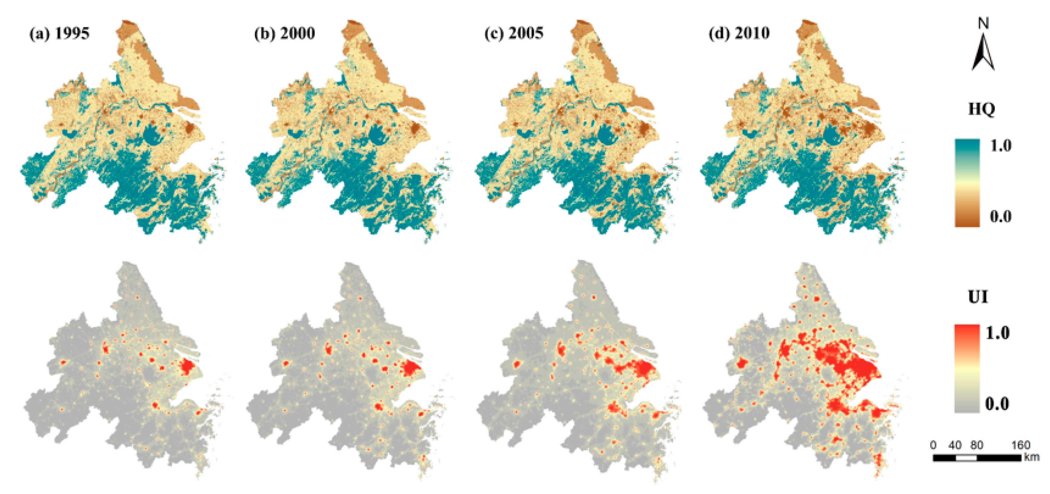
3.1. The HQ and UI Spatiotemporal Variations in YRDUA

3.1.1. The Spatial and Temporal Changes in Habitat Quality

Habitat quality and urbanization intensity maps have different spatial patterns across YRDUA (Figure 2). The HQ varied from 0 to 1 for the four time periods analyzed. With two clearly isolated high-value areas corresponding to Huangshan Mountain and the Taihu Lake, the HQ values were generally higher along the southwestern mountains in Zhejiang Province and decreased in the northeastern plains in Jiangsu Province. Furthermore, the lowest HQ values were concentrated around the major urban areas of Shanghai, Suzhou, Nanjing and Wuxi, which have the highest population densities. Among the different land use types, forestland was the main provider of HQ in YRDUA, followed by cultivated land and water bodies. HQ was lower in urban areas than it was in the other land cover types. This is mainly due to the small amount of ecological land resulting from the large quantities of construction land, leading to a decline in the total habitat quality.
With a decreasing rate of 4.95% (Table 2), the average values of regional HQ were 0.586, 0.581, 0.572 and 0.557 in 1995, 2000, 2005 and 2010, respectively. HQ decreased not only on a regional scale, but also in 23 cities of YRDUA, the largest of which was Shanghai (−18.83%), followed by Suzhou (−17.19%). HQ increased slightly only for Chuzhou, Xuancheng and Anqing, by 0.98%, 0.31% and 0.12%, respectively (Figure 3). In terms of jurisdictions, the change in HQ in Suzhou was the most substantial (−0.098), while the lowest amount of change was found in Chuzhou (0.005). The average HQ was highest in Hangzhou (0.79) and lowest in Shanghai (0.27) in 2010.

3.1.2. The Spatial and Temporal Changes in Urbanization Intensity

The spatial distribution pattern of UI in YRDUA was opposite to that of HQ (Figure 2). UI was the highest along the Yangtze River and Hangzhou Bay, especially in the Yangtze River Estuary (Shanghai, Suzhou and Wuxi), where urbanization gradually decreased from the center to the outskirts. As an important ecological barrier and drinking water source for YRDUA, a variety of ecological protection projects were implemented in the southwestern region; therefore, the UI was relatively low compared with that in other places. With a rate of increase of 177.56%, the average value of regional UI was 0.092, 0.109, 0.134, and 0.256 in 1995, 2000, 2005 and 2010, respectively. In 2010, the average value of UI was highest in Shanghai (0.723), followed by Xuancheng (0.062), Anqing (0.063) and Chizhou (0.056) (Figure 4). Suzhou, which had the largest decrease in HQ, was also the most prominent city for the increase in urbanization (0.456), while Anqing had the smallest decrease (0.045).

3.2. The Relationship between HQ and UI

3.2.1. Regional Scale

To identify the threat level of UI to HQ in each pixel, the spatial pattern of the descending rate ( Q ) between UI and HQ was analyzed among all the periods (Figure 5). Overall, HQ was negatively correlated with UI, i.e., the regression coefficients in all the regional pixels were less than zero. The threat level from the urban center to the outskirts is a “reverse U” trend, which is enhanced after the decrease. The minimum negative urbanization impact on HQ, which was mainly distributed in the surrounding suburban area, covered nearly 50% of the urbanization range ( β = 0.2 ~ 0.7 ), while Q o b s declined significantly with increasing UI in the urban core districts (Shanghai, Suzhou, Wuxi, Changzhou, Nanjing, Hangzhou and Hefei) and unfrequented areas. Similar to the mountains surrounding the urban center, along the sides of the ridge, the impact of urbanization on HQ gradually increased. In the temporal gradients, each threat level was continuously pushed outward and closer together until they merged into a larger multicenter band, such as the Hangzhou Bay Belt, the Yangtze River Estuary and the Yangtze River Belt. This was consistent with the result of the polycentric megaregion evolution model in previous studies [49].
Based on the kernel density distribution of HQ, the Q m e a n had a distinct nonlinear relationship with UI (p < 0.001) along the urban-rural gradients of YRDUA (Figure 5). There were two inflection points in the relationship between HQ and UI. In the position where the urbanization was 20%, the response of HQ to UI changed from a steady decrease to stable. However, when urbanization reached 80%, HQ went from stable back to a steady decrease. In the early period, only some pixels with low Q o b s gradually evolved to a higher UI. Over time, the urbanized level of areas with a high value of Q o b s started to increase, and the medium value of Q o b s appeared in all the urbanization gradients, even in extremely highly urbanized areas. The transformation in the relationship indicated that more natural areas were affected by urbanization and that the habitat quality in urban areas was improved in the process of urbanization.

3.2.2. City Scale

The relationships between UI and HQ across cities in YRDUA in 2010 are shown in Figure 6, and the results for other years in Figures S2–S4. Generally, HQ decreased with the enhancement of urbanization in each city, because the proportion of vegetation types in the grids was gradually replaced by built-up areas along the range of urbanization. Comparing the relationship curves of various cities, 15% of cities, such as Chizhou, Wuxi, Ningbo, and Suzhou, were linearly and negatively correlated. Seventy percent of cities, such as Tongling, Nanjing, and Hangzhou, have the same nonlinear relationship as that of the regional scale. Nevertheless, there were some exceptions, such as Nantong, Shanghai, Yancheng and Jiaxing, where HQ was not significantly negatively correlated with UI. The HQ maintained a relatively consistent value in areas of moderate urbanization. Different forms of the relationships were largely related to the local development orientation and urbanization level. The background value of each city may be associated with the local natural background and climatic conditions.

3.3. The Direct and Indirect Impacts of Urbanization on HQ

3.3.1. Regional Urbanization Impacts on HQ

The preliminary findings showed that Q o b s and Q d , which showed nonlinear and linear variation, respectively, declined along the UI gradient across cities (Figure 7a,b). Some UI gradients were empty (i.e., β = 0.0317   and   0.0476 ) because the DN values of 2 and 3 were not found in the DMSP-OLS NTL data for YRDUA. To study the reason for the difference between the nonlinear relationship and the linear relationship, the part of the HQ variation under indirect impacts was separately extracted and studied (Figure 7c). The indirect impact of HQ ( Q i d ) (i.e., below zero) was mainly concentrated in the early stage of urbanization, and the Q i d in moderate-high UI was above the zero-impact line, with a maximum value of β = 0.8. As shown in Figure 7d, the relative contribution coefficient ( τ ) was negative at values less than β = 0.4 and tended to stabilize after growth beyond zero, which indicated that urbanization in the primary stage has a negative indirect impact on local HQ, but at a relatively high urbanization level, it gradually turned into a positive impact. Conceptually, a negative indirect impact will accelerate habitat degradation, while a positive indirect impact can partially offset the habitat degradation caused by land conversion. The average offset extent was approximately 28.23%, 17.41%, 22.94%, and 16.18% in 1995, 2000, 2005, and 2010, respectively. Notably, the variation in τ was more significant in areas of lower urbanization intensity because the observed HQs were higher than the background HQ value in pixels with relatively low urban intensity, especially for highly ecologically sensitive areas.

3.3.2. Urbanization Impacts on HQ in Cities

It is worth mentioning that the HQ value of almost all the pixels in the areas with relatively high urbanization intensity was above the zero-impact line for 26 cities, which indicated the positive ecological impact of urbanization in the urban environment. The median of the observed habitat quality ( Q m e a n ), the background habitat quality index ( Q b ) and the mean of the medians of the relative contribution coefficient (τ) in all the urban pixels for 26 cities in YRDUA for the period of 1995 to 2010 are shown in Tables S2–S5. For example, the median observed HQ among all the pixels of Ningbo was 0.53, and the Q b was 0.80, which offset 22.21% of the loss of habitat quality through vegetation cover reduction in 2010. The observed HQ in some pixels, which was even larger than the background value, caused a higher offset of HQ, such as 54.34% in Yancheng and 53.98% in Hefei in 2010.

4. Discussion

4.1. Nonlinear Relationship between Habitat Quality and Urbanization Intensity

Based on land use [55], urban populations [26] and impervious surfaces [56], the overall ecological urbanization impact on HQ was negative. Nighttime light data serve as the composite response to the interaction of these factors and were used to characterize the overall urbanization intensity [57]. We found that the nonlinear negative relationship between HQ and UI changed from a steady decrease to stable and then back to a steady decrease, with inflection points where urbanization reaches 20% and 80%. The transformation in the relationship indicated that more natural areas were affected by urbanization, and the habitat quality in urban areas was improved in the process of urbanization, which was consistent with the results of previous research. The ecological conditions in 20% of YRDUA deteriorated, and the ecological conditions in 40% increased from 1995 to 2010 [19]. The improvement in habitat quality in urban areas has also been testified in accelerating vegetation growth [21,22,58] and enhancing species richness [18,20] in urban environments compared to those in rural equivalents.
Habitat quality is used as a surrogate to assess the status of extant biodiversity under human activities [59]. Different dynamics of HQ were largely dominated by local ecological factors and complex land use patterns (Figure 8). In woodland areas, the ecosystem structures were more complicated to support the survival and reproduction of relatively diverse species. In contrast, under intensive human intervention, cultivated land represents poor habitat, hosting relatively few species, which is equivalent to urban areas [60]. In rural areas of YRDUA ( β < 0.2), land use was bifurcated into woodland and cropland, which established completely different ecological backgrounds. We also found some cities, such as Changzhou, Nanjing, Nantong, Taizhou, Yancheng, Wuxi, Zhenjiang, Shanghai and Jiaxing, where the HQ dynamics were relatively consistent in moderate or even higher UI. Cropland (53–85%) accounted for the majority of the land cover in these cities and had stable relationships, while woodland accounted for less than 10%, leading to landscape homogenization from the city center to the outskirts ( β = 0.2~0.8), with a relatively consistent habitat quality. At an extremely high urbanization level ( β > 0.8), urban land use was mainly converted from cultivated land to urban land, resulting in a drastic reduction in habitat quality. The same relationship type has also been proposed in corresponding studies of plant diversity [61], birds [43] and amphibian abundance [17].

4.2. The Necessity of Distinguishing Urbanization Impacts on Habitat Quality

Some existing studies focused on overall impact rather than distinguishing the urbanization effect into direct impact and indirect impacts [22,62,63]. Although the habitat in YRDUA degenerated with urbanization growth, the HQ of the urban area increased during the urbanization process (Figure 7). The reduction in HQ was the result of ecological land being occupied by constructed land, while the remaining habitats in the urban areas retained relatively good ecological conditions. The impact of urbanization on HQ is difficult to fully explain with the replacement of ecological land, which was also related to human demands in different urbanization stages [46]. Therefore, analyzing and quantifying the direct and indirect impacts of urbanization on HQ dynamics is necessary.
The cities in YRDUA have varying urbanization stages, and the impact of urbanization on HQ was also different. Based on the variations in HQ, UI and τ , the cities can be divided into four clusters (Figure 9). (I) A total of 11.5% of the cities, including Jiaxing, Wuhu and Maanshan, were in the first category, which was characterized by relatively low HQ values and an exacerbated rate of habitat degradation as a result of urbanization. (II) A total of 42.3% of the cities, including Nantong, Zhoushan, and Huzhou, were in the second category, which had relatively low HQ values and habitat degradation. (III) A total of 34.6% of the cities, including Wuxi and Suzhou, were in the third category, which had a relatively high HQ. In this category, the habitat degradation was offset by urbanization. (IV) Approximately 11.5% of the cities, including Shanghai, Nanjing and Zhenjiang, were in the fourth category, which had slightly improved HQ values. Urbanization still exacerbated habitat degradation in this category.
The diversity of the demands created by human beings in different urbanization stages impacts the approach used to manage landscapes [46,64]. Based on this study, the indirect urbanization impact on habitat quality dynamics was categorized into four stages: the damage stage (I), antagonistic stage (II), coordination stage (III), and degenerative stage (IV). The indirect urbanization impact was distinguished as negative impacts and positive impacts (Figure 10). In the damage stage, the negative impact on habitats increased significantly at low urbanization levels due to patch fragmentation, a shortage in the food supply, and a weakening of ecosystem resistance and resilience. Resource exploitation (e.g., deforestation and overkilling) also destroyed the ecological conditions in the available habitat. In the second stage, rapid urbanization accelerated the occupation of ecological land. At the same time, some ecological protection and restoration works were applied to match the urgent demand for blue-green ecological space (e.g., green space and aquatic landscapes) and corresponding ecosystem services. In the coordination stage, with awareness about human ecological protection and continuous investment in ecological restoration and management, some key ecological corridors and functions had been repaired, and the positive ecological impacts caused by urbanization had gradually offset the negative impacts [64]. In the degenerative stage, the extremely high proportion of built-up areas provided very limited space for species to thrive, which increased the hazard exposure of species to the external environment. The positive ecological utility generated by manual management had a threshold and could not be increased without limitation. The negative impact from the surrounding environment increased persistently, resulting in a certain degree of reduction in comprehensive utility.

4.3. Limitations and Future Directions

Although the application of the InVEST model to regional biodiversity conservation has proven to be effective, the assessment of HQ has limitations related to two factors: the accuracy of the land cover data and the impact threshold of the threat factors. In the estimation of HQ in YRDUA, 30 m resolution land cover data were used and separated into 17 categories, and the variation in habitat types was not sensitive at some lower scales with small patches. This may obscure the complexity of the habitat, especially in Zhoushan, a city of multiple islands. Moreover, the isolated habitat fragments present in urban areas often maintain different plant and insect communities, but they are most likely only visited by individuals of the same widespread avian and mammal species. In our study, we used a relatively small impact threshold ( i r x y ) for each threat factor used to calculate HQ, which is more appropriate for species such as plants, invertebrates, and small mammals, which have a range of survival activities less than or equal to this value. In reality, the assessment of large-scale HQ often contains uncertainty in its results due to the lack of corresponding observation data. Moreover, the quality of the data is related to the issues that need to be addressed in the research. Although the remote sensing approach to assessing HQ may simplify the understanding of complex ecological processes, our study aims to analyze the prevalent dynamics of habitats in urbanization gradients to achieve the vision of broad protection of biodiversity in rapid urbanization. It involves the protection of not one species or community but multiple positive elements in a habitat (e.g., habitat quality, ecological carrying capacity, and biodiversity) and the identification and control of threats that may cause damage to habitats.
The urbanization characterized by NTL data could also create uncertainty. Urbanization can be represented by economic aggregation and residential expansion, which is also related to the variation in the NTL data. However, the quantitative relationship between nighttime light data and various urbanization indicators is not well understood [27]. The variation in NTL data may reflect the spatial and aggregation statuses of economies and populations in YRDUA, although it was not consistent with the actual urbanization at the pixel level [65]. The 1 km spatial resolution DMSP-OLS dataset spans two decades (1992–2013), which leads to limited timeliness and spatial precision in this study. The coarse resolution and blooming effect of DMSP-OLS NTL data require future improvements in the accuracy of extracting urbanization information. The NPP-VIIRS NTL data collected on the Suomi satellite have relatively high resolution and no pixel oversaturation; therefore, they could be used for a higher quality evaluation of urbanization.
In general, although there is some uncertainty in the data sources, from a macro perspective, our study is still valuable for the exploration of the ecological impact of different urbanization stages on terrestrial ecosystems. Therefore, to achieve a more in-depth picture of the ecological impacts of various urbanization stages on habitats, multisource, higher-resolution datasets (e.g., Quickbird images and NPP-VIIRS NTL data) will be used, and field observation experiments will be added to lessen the uncertainty of assessment results from remote sensing approaches.

5. Conclusions

In this study, the relationship between HQ and UI and the direct and indirect impacts of urbanization on HQ were delineated and analyzed for YRDUA from 1995 to 2010 through the application of remote sensing data. The results indicated that urbanization might lead to habitat degradation, while awareness about protecting ecological conditions began to increase after the antagonistic stage of urbanization. The main conclusions can be summarized as follows:
  • The YRDUA underwent rapid urbanization from 1995 to 2010, intensifying urban expansion and human activities. The vast majority of urban expansion was concentrated in the Hangzhou Bay Belt, the Yangtze River Estuary and the Yangtze River Belt, accompanied by a large proportion of habitat degradation.
  • The overall dynamic of HQ was generally nonlinear and negative along the urbanization gradient, whereas the nonlinear negative relationship between HQ and UI changed from a steady decrease to stable and then back to a steady decrease, with inflection points where urbanization reached 20% and 80%. The transformation in the relationship indicated that more natural areas were affected by urbanization and that the habitat quality in urban areas was improved in the process of urbanization.
  • With an improved conceptual framework, the difference between linear and nonlinear relationships depends on the indirect urbanization impact. Negative indirect impacts will accelerate habitat degradation, while positive impacts can partially offset habitat degradation caused by land conversion. The average offset extent was approximately 28.23%, 17.41%, 22.94%, and 16.18% in 1995, 2000, 2005, and 2010, respectively. Nearly 76.9% of the cities showed positive indirect impacts, and 55% of them showed improved habitat quality.

Supplementary Materials

Author Contributions

Conceptualization, J.Z. and N.D.; methodology, J.Z., N.D. and Y.X.; software, J.Z. and D.L.; validation, J.Z., and D.L.; formal analysis, J.Z.; resources, W.S.; data curation, J.Z. and D.L.; writing—original draft preparation, J.Z.; writing—review and editing, J.Z., W.S. and Y.X.; visualization, J.Z.; supervision, X.W. and Y.X.; project administration, X.W.; funding acquisition, X.W. All authors have read and agreed to the published version of the manuscript.

Funding

This research was funded by the National Key Research and Development Program of China (Grant No. 2016YFC0502700) and the National Social Science Major Foundation of China (Grant No. 14ZDB140).

Conflicts of Interest

The authors declare no conflict of interest.

References

  1. Li, C.; Li, J.X.; Wu, J.G. Quantifying the speed, growth modes, and landscape pattern changes of urbanization: A hierarchical patch dynamics approach. Landsc. Ecol. 2013, 28, 1875–1888. [Google Scholar] [CrossRef]
  2. Liu, Z.F.; He, C.Y.; Zhou, Y.Y.; Wu, J.G. How much of the world’s land has been urbanized, really? A hierarchical framework for avoiding confusion. Landsc. Ecol. 2014, 29, 763–771. [Google Scholar] [CrossRef]
  3. Huang, G.L.; Zhou, W.Q.; Cadenasso, M.L. Is everyone hot in the city? Spatial pattern of land surface temperatures, land cover and neighborhood socioeconomic characteristics in Baltimore, MD. J. Environ. Manag. 2011, 92, 1753–1759. [Google Scholar] [CrossRef]
  4. Grimm, N.B.; Faeth, S.H.; Golubiewski, N.E.; Redman, C.L.; Wu, J.G.; Bai, X.M.; Briggs, J.M. Global change and the ecology of cities. Science 2008, 319, 756–760. [Google Scholar] [CrossRef] [Green Version]
  5. Islam, K.R.; Weil, R.R. Land use effects on soil quality in a tropical forest ecosystem of Bangladesh. Agric. Ecosyst. Environ. 2000, 79, 9–16. [Google Scholar] [CrossRef]
  6. Zhou, W.Q.; Qian, Y.G.; Li, X.M.; Li, W.F.; Han, L.J. Relationships between land cover and the surface urban heat island: Seasonal variability and effects of spatial and thematic resolution of land cover data on predicting land surface temperatures. Landsc. Ecol. 2014, 29, 153–167. [Google Scholar] [CrossRef]
  7. He, C.Y.; Liu, Z.F.; Tian, J.; Ma, Q. Urban expansion dynamics and natural habitat loss in China: A multiscale landscape perspective. Glob. Chang. Biol. 2014, 20, 2886–2902. [Google Scholar] [CrossRef]
  8. Pickett, S.T.A.; Cadenasso, M.L.; Grove, J.M.; Boone, C.G.; Groffman, P.M.; Irwin, E.; Kaushal, S.S.; Marshall, V.; McGrath, B.P.; Nilon, C.H.; et al. Urban ecological systems: Scientific foundations and a decade of progress. J. Environ. Manag. 2011, 92, 331–362. [Google Scholar] [CrossRef] [PubMed]
  9. Carreiro, M.M.; Tripler, C.E. Forest remnants along urban-rural gradients: Examining their potential for global change research. Ecosystems 2005, 8, 568–582. [Google Scholar] [CrossRef]
  10. Youngsteadt, E.; Dale, A.G.; Terando, A.J.; Dunn, R.R.; Frank, S.D. Do cities simulate climate change? A comparison of herbivore response to urban and global warming. Glob. Chang. Biol. 2015, 21, 97–105. [Google Scholar] [CrossRef]
  11. McDonnell, M.J.; Pickett, S.T.A. Ecosystem structure and function along urban rural gradients—An unexploited opportunity for ecology. Ecology 1990, 71, 1232–1237. [Google Scholar] [CrossRef]
  12. Saunders, M.I.; Atkinson, S.; Klein, C.J.; Weber, T.; Possingham, H.P. Increased sediment loads cause non-linear decreases in seagrass suitable habitat extent. PLoS ONE 2017, 12, 21. [Google Scholar] [CrossRef] [PubMed] [Green Version]
  13. Isbell, F.; Gonzalez, A.; Loreau, M.; Cowles, J.; Diaz, S.; Hector, A.; Mace, G.M.; Wardle, D.A.; O’Connor, M.I.; Duffy, J.E.; et al. Linking the influence and dependence of people on biodiversity across scales. Nature 2017, 546, 65–72. [Google Scholar] [CrossRef] [PubMed] [Green Version]
  14. Mimura, M.; Yahara, T.; Faith, D.P.; Vazquez-Dominguez, E.; Colautti, R.I.; Araki, H.; Javadi, F.; Nunez-Farfan, J.; Mori, A.S.; Zhou, S.L.; et al. Understanding and monitoring the consequences of human impacts on intraspecific variation. Evolut. Appl. 2017, 10, 121–139. [Google Scholar] [CrossRef] [PubMed]
  15. Aronson, M.F.J.; La Sorte, F.A.; Nilon, C.H.; Katti, M.; Goddard, M.A.; Lepczyk, C.A.; Warren, P.S.; Williams, N.S.G.; Cilliers, S.; Clarkson, B.; et al. A global analysis of the impacts of urbanization on bird and plant diversity reveals key anthropogenic drivers. Proc. R. Soc. B Biol. Sci. 2014, 281, 8. [Google Scholar] [CrossRef]
  16. Pregitzer, C.C.; Charlop-Powers, S.; Bibbo, S.; Forgione, H.M.; Gunther, B.; Hallett, R.A.; Bradford, M.A. A city-scale assessment reveals that native forest types and overstory species dominate New York City forests. Ecol. Appl. 2019, 29, 12. [Google Scholar] [CrossRef]
  17. Jennette, M.A.; Snodgrass, J.W.; Forester, D.C. Variation in age, body size, and reproductive traits among urban and rural amphibian populations. Urban Ecosyst. 2019, 22, 137–147. [Google Scholar] [CrossRef]
  18. Thomas, J.P.; Jung, T.S. Life in a northern town: Rural villages in the boreal forest are islands of habitat for an endangered bat. Ecosphere 2019, 10, 15. [Google Scholar] [CrossRef] [Green Version]
  19. Meng, Z.; Liu, M.; She, Q.; Yang, F.; Long, L.; Peng, X.; Han, J.; Xiang, W. Spatiotemporal Characteristics of Ecological Conditions and Its Response to Natural Conditions and Human Activities during 1990(–)2010 in the Yangtze River Delta, China. Int. J. Environ. Res. Public Health 2018, 15, 2910. [Google Scholar] [CrossRef] [Green Version]
  20. McKinney, M.L. Effects of urbanization on species richness: A review of plants and animals. Urban Ecosyst. 2008, 11, 161–176. [Google Scholar] [CrossRef]
  21. Jia, W.X.; Zhao, S.Q.; Liu, S.G. Vegetation growth enhancement in urban environments of the Conterminous United States. Glob. Chang. Biol. 2018, 24, 4084–4094. [Google Scholar] [CrossRef]
  22. Zhao, S.Q.; Liu, S.G.; Zhou, D.C. Prevalent vegetation growth enhancement in urban environment. Proc. Natl. Acad. Sci. USA 2016, 113, 6313–6318. [Google Scholar] [CrossRef] [PubMed] [Green Version]
  23. Dobbs, C.; Nitschke, C.; Kendal, D. Assessing the drivers shaping global patterns of urban vegetation landscape structure. Sci. Total Environ. 2017, 592, 171–177. [Google Scholar] [CrossRef] [PubMed]
  24. Ossola, A.; Hopton, M.E. Climate differentiates forest structure across a residential macrosystem. Sci. Total Environ. 2018, 639, 1164–1174. [Google Scholar] [CrossRef] [PubMed]
  25. Polasky, S.; Nelson, E.; Pennington, D.; Johnson, K.A. The Impact of Land-Use Change on Ecosystem Services, Biodiversity and Returns to Landowners: A Case Study in the State of Minnesota. Environ. Resour. Econ. 2011, 48, 219–242. [Google Scholar] [CrossRef]
  26. Peng, J.; Tian, L.; Liu, Y.X.; Zhao, M.Y.; Hu, Y.N.; Wu, J.S. Ecosystem services response to urbanization in metropolitan areas: Thresholds identification. Sci. Total Environ. 2017, 607, 706–714. [Google Scholar] [CrossRef]
  27. Elvidge, C.D.; Sutton, P.C.; Baugh, K.E.; Ziskin, D.C.; Anderson, S. National Trends in Satellite Observed Lighting: 1992–2009. In AGU Fall Meeting Abstracts; AGU: Washington, DC, USA, 2011. [Google Scholar]
  28. Shi, K.F.; Huang, C.; Yu, B.L.; Yin, B.; Huang, Y.X.; Wu, J.P. Evaluation of NPP-VIIRS night-time light composite data for extracting built-up urban areas. Remote Sens. Lett. 2014, 5, 358–366. [Google Scholar] [CrossRef]
  29. Liu, Z.F.; He, C.Y.; Zhang, Q.F.; Huang, Q.X.; Yang, Y. Extracting the dynamics of urban expansion in China using DMSP-OLS nighttime light data from 1992 to 2008. Landsc. Urban Plan. 2012, 106, 62–72. [Google Scholar] [CrossRef]
  30. Zhou, Y.Y.; Smith, S.J.; Elvidge, C.D.; Zhao, K.G.; Thomson, A.; Imhoff, M. A cluster-based method to map urban area from DMSP/OLS nightlights. Remote Sens. Environ. 2014, 147, 173–185. [Google Scholar] [CrossRef]
  31. Gallo, K.P.; Tarpley, J.D.; McNab, A.L.; Karl, T.R. Assessment of urban heat islands—A satellite perspective. Atmos. Res. 1995, 37, 37–43. [Google Scholar] [CrossRef]
  32. Propastin, P.; Kappas, M. Assessing Satellite-Observed Nighttime Lights for Monitoring Socioeconomic Parameters in the Republic of Kazakhstan. GISci. Remote Sens. 2012, 49, 538–557. [Google Scholar] [CrossRef]
  33. Fan, J.F.; Ma, T.; Zhou, C.H.; Zhou, Y.K.; Xu, T. Comparative Estimation of Urban Development in China’s Cities Using Socioeconomic and DMSP/OLS Night Light Data. Remote Sens. 2014, 6, 7840–7856. [Google Scholar] [CrossRef] [Green Version]
  34. Wu, J.S.; Wang, Z.; Li, W.F.; Peng, J. Exploring factors affecting the relationship between light consumption and GDP based on DMSP/OLS nighttime satellite imagery. Remote Sens. Environ. 2013, 134, 111–119. [Google Scholar] [CrossRef]
  35. Chand, T.R.K.; Badarinath, K.V.S.; Elvidge, C.D.; Tuttle, B.T. Spatial characterization of electrical power consumption patterns over India using temporal DMSP-OLS night-time satellite data. Int. J. Remote Sens. 2009, 30, 647–661. [Google Scholar] [CrossRef]
  36. Davies, T.W.; Bennie, J.; Inger, R.; De Ibarra, N.H.; Gaston, K.J. Artificial light pollution: Are shifting spectral signatures changing the balance of species interactions? Glob. Chang. Biol. 2013, 19, 1417–1423. [Google Scholar] [CrossRef] [Green Version]
  37. Milesi, C.; Elvidge, C.D.; Nemani, R.R.; Running, S.W. Assessing the impact of urban land development on net primary productivity in the southeastern United States. Remote Sens. Environ. 2003, 86, 401–410. [Google Scholar] [CrossRef]
  38. Imhoff, M.L.; Tucker, C.J.; Lawrence, W.T.; Stutzer, D.C. The use of multisource satellite and geospatial data to study the effect of urbanization on primary productivity in the United States. IEEE Trans. Geosci. Remote Sens. 2000, 38, 2549–2556. [Google Scholar]
  39. Wang, J.L.; Zhou, W.Q.; Pickett, S.T.A.; Yu, W.J.; Li, W.F. A multiscale analysis of urbanization effects on ecosystem services supply in an urban megaregion. Sci. Total Environ. 2019, 662, 824–833. [Google Scholar] [CrossRef]
  40. Maes, J.; Paracchini, M.L.; Zulian, G.; Dunbar, M.B.; Alkemade, R. Synergies and trade-offs between ecosystem service supply, biodiversity, and habitat conservation status in Europe. Biol. Conserv. 2012, 155, 1–12. [Google Scholar] [CrossRef]
  41. Li, B.; Zhang, W.; Shu, X.X.; Pei, E.L.; Yuan, X.; Wang, T.H.; Wang, Z.H. Influence of breeding habitat characteristics and landscape heterogeneity on anuran species richness and abundance in urban parks of Shanghai, China. Urban For. Urban Green. 2018, 32, 56–63. [Google Scholar] [CrossRef]
  42. Sun, X.; Crittenden, J.C.; Li, F.; Lu, Z.M.; Dou, X.L. Urban expansion simulation and the spatio-temporal changes of ecosystem services, a case study in Atlanta Metropolitan area, USA. Sci. Total Environ. 2018, 622, 974–987. [Google Scholar] [CrossRef] [PubMed]
  43. Blair, R.B.; Johnson, E.M. Suburban habitats and their role for birds in the urban-rural habitat network: Points of local invasion and extinction? Landsc. Ecol. 2008, 23, 1157–1169. [Google Scholar] [CrossRef]
  44. Terrado, M.; Sabater, S.; Chaplin-Kramer, B.; Mandle, L.; Ziv, G.; Acuna, V. Model development for the assessment of terrestrial and aquatic habitat quality in conservation planning. Sci. Total Environ. 2016, 540, 63–70. [Google Scholar] [CrossRef] [PubMed] [Green Version]
  45. Sun, C.Z.; Zhen, L.; Wang, C.; Yan, B.Y.; Cao, X.C.; Wu, R.Z. Impacts of ecological restoration and human activities on habitat of overwintering migratory birds in the wetland of Poyang Lake, Jiangxi Province, China. J. Mount. Sci. 2015, 12, 1302–1314. [Google Scholar] [CrossRef]
  46. Yi, L.; Chen, J.; Jin, Z.; Quan, Y.; Han, P.; Guan, S.; Jiang, X. Impacts of human activities on coastal ecological environment during the rapid urbanization process in Shenzhen, China. Ocean Coast. Manag. 2018, 154, 121–132. [Google Scholar] [CrossRef]
  47. Guan, X.B.; Shen, H.F.; Li, X.H.; Gan, W.X.; Zhang, L.P. A long-term and comprehensive assessment of the urbanization-induced impacts on vegetation net primary productivity. Sci. Total Environ. 2019, 669, 342–352. [Google Scholar] [CrossRef]
  48. Cidell, J. Concentration and decentralization: The new geography of freight distribution in US metropolitan areas. J. Transp. Geogr. 2010, 18, 363–371. [Google Scholar] [CrossRef]
  49. Feng, Y.H.; Wu, S.F.; Wu, P.X.; Su, S.L.; Weng, M.; Bian, M. Spatiotemporal characterization of megaregional poly-centrality: Evidence for new urban hypotheses and implications for polycentric policies. Land Use Policy 2018, 77, 712–731. [Google Scholar] [CrossRef]
  50. Yangtze River Delta Yearbook (YRDY); Hohai University Press: Shanghai, China, 2015.
  51. Zhang, D.; Qu, L.P.; Zhang, J.H. Ecological security pattern construction method based on the perspective of ecological supply and demand: A case study of Yangtze River Delta. Acta Ecol. Sin. 2019, 39, 13. [Google Scholar]
  52. Sharp, R.; Tallis, H.T.; Ricketts, T.; Guerry, A.D.; Wood, S.A.; Chaplin-Kramer, R.; Nelson, E.; Ennaanay, D.; Wolny, S.; Olwero, N.; et al. VEST 3.3.1 User’s Guide; The Natural Capital Project: Stanford, CA, USA, 2016. [Google Scholar]
  53. Chen, J.; Zhuo, L.; Shi, P.; Ichinose, T. A study of the urbanization process in China based on DMSP/OLS data: Development of a light index for urbanization level estimation. J. Remote Sens. 2003, 7, 168–175, 241. [Google Scholar]
  54. Yang, M.; Wang, S.X.; Zhou, Y.; Wang, L.T. A Method of Urbanization Level Estimation Using DMSP/OLS Imagery. Remote Sens. Inf. 2011, 26, 100–106. [Google Scholar]
  55. Sallustio, L.; De Toni, A.; Strollo, A.; Di Febbraro, M.; Gissi, E.; Casella, L.; Geneletti, D.; Munafo, M.; Vizzarri, M.; Marchetti, M. Assessing habitat quality in relation to the spatial distribution of protected areas in Italy. J. Environ. Manag. 2017, 201, 129–137. [Google Scholar] [CrossRef] [PubMed]
  56. Helms, B.S.; Feminella, J.W.; Pan, S. Detection of biotic responses to urbanization using fish assemblages from small streams of western Georgia, USA. Urban Ecosyst. 2005, 8, 39–57. [Google Scholar] [CrossRef]
  57. Li, X.; Zhou, Y. Urban mapping using DMSP/OLS stable night-time light: A review. Int. J. Remote Sens. 2017, 38, 6030–6046. [Google Scholar] [CrossRef]
  58. Pretzsch, H.; Biber, P.; Uhl, E.; Dahlhausen, J.; Schutze, G.; Perkins, D.; Rotzer, T.; Caldentey, J.; Koike, T.; van Con, T.; et al. Climate change accelerates growth of urban trees in metropolises worldwide. Sci. Rep. 2017, 7, 10. [Google Scholar] [CrossRef] [PubMed]
  59. Stephens, P.A.; Pettorelli, N.; Barlow, J.; Whittingham, M.J.; Cadotte, M.W. Management by proxy? The use of indices in applied ecology. J.Appl. Ecol. 2015, 52, 1–6. [Google Scholar] [CrossRef]
  60. Gamez-Virues, S.; Perovic, D.J.; Gossner, M.M.; Borsching, C.; Bluthgen, N.; de Jong, H.; Simons, N.K.; Klein, A.M.; Krauss, J.; Maier, G.; et al. Landscape simplification filters species traits and drives biotic homogenization. Nat. Commun. 2015, 6, 8. [Google Scholar] [CrossRef]
  61. Yan, Z.G.; Teng, M.J.; He, W.; Liu, A.Q.; Li, Y.R.; Wang, P.C. Impervious surface area is a key predictor for urban plant diversity in a city undergone rapid urbanization. Sci. Total Environ. 2019, 650, 335–342. [Google Scholar] [CrossRef]
  62. Xie, W.X.; Huang, Q.X.; He, C.Y.; Zhao, X. Projecting the impacts of urban expansion on simultaneous losses of ecosystem services: A case study in Beijing, China. Ecol. Indic. 2018, 84, 183–193. [Google Scholar] [CrossRef]
  63. Li, Y.; Zhao, S.Q.; Zhao, K.; Xie, P.; Fang, J.Y. Land-cover changes in an urban lake watershed in a mega-city, Central China. Environ. Monit. Assess. 2006, 115, 349–359. [Google Scholar] [CrossRef]
  64. Peng, J.; Shen, H.; Wu, W.H.; Liu, Y.X.; Wang, Y.L. Net primary productivity (NPP) dynamics and associated urbanization driving forces in metropolitan areas: A case study in Beijing City, China. Landsc. Ecol. 2016, 31, 1077–1092. [Google Scholar] [CrossRef]
  65. Zhou, C.; Wang, S.; Wang, J. Examining the influences of urbanization on carbon dioxide emissions in the Yangtze River Delta, China: Kuznets curve relationship. Sci. Total Environ. 2019, 675, 472–482. [Google Scholar] [CrossRef] [PubMed]
Figure 1. The Yangtze River Delta Urban Agglomeration (YRDUA) study location in China showing the topography and expansion of built-up areas during 1995–2010.
Sustainability 12 00669 g001
Figure 2. Spatial patterns of habitat quality and urbanization intensity in different years in YRDUA. (a) 1995, (b) 2000, (c) 2005, and (d) 2010.
Sustainability 12 00669 g002
Figure 3. (a) Annual average value of HQ and (b) the variation in HQ in YRDUA from 1995 to 2010.
Sustainability 12 00669 g003
Figure 4. (a) Annual average value of UI and (b) the variation in UI in YRDUA from 1995 to 2010.
Sustainability 12 00669 g004
Figure 5. Spatial pattern of Q (threat level of UI to HQ) and kernel density distribution of Q o b s in each UI gradient in 1995–2010 in YRDUA. The red curve is the cubic polynomial fit of Q m e a n to UI. (a) 1995, (b) 2000, (c) 2005, and (d) 2010.
Sustainability 12 00669 g005
Figure 6. The relationship between UI and HQ across 26 cities in YRDUA in 2010. The red line represents the polynomial fitting curve of Q obs in each scatter diagram, and the straight blue line represents the zero-impact line. The HQ responses to UI for 1995, 2000 and 2005 are shown in Figures S3–S5.
Sustainability 12 00669 g006
Figure 7. The relationship between UI and HQ for YRDUA in 2010: (a) the observed HQ along the UI   gradients ( Q o b s ); (b) the direct HQ value change ( Q d ); (c) the indirect HQ change ( Q i d ), in which the indirect growth of HQ peaked at approximately 0.8, indicated by the red dotted line; and (d) the relative contribution coefficient ( τ ) . The boxplot for τ in each box shows 25% and 75% (the black points are outliers, the medians for each box are marked by the orange points, and the mean of the medians is 16.18%, as shown by the red lines).
Sustainability 12 00669 g007
Figure 8. The proportion of each land cover type with UI gradients in YRDUA in 2010.
Sustainability 12 00669 g008
Figure 9. The variation in the median observed habitat quality ( Q m e a n ), urbanization intensity ( β ) and the offset of habitat degradation ( τ ) of 26 cities in YRDUA from 1995 to 2010.
Sustainability 12 00669 g009
Figure 10. The urbanization stages and their indirect impacts on HQ dynamics. The dotted red line represents the upper limit of the positive impacts.
Sustainability 12 00669 g010
Table 1. Weight combination of nighttime light intensity index (NLII) and nighttime light area index (NLAI).
Number p 1 p 2 Weight Combination
101NLAI
20.10.90.1 NLII + 0.9 NLAI
30.20.80.2 NLII + 0.8 NLAI
40.30.70.3 NLII + 0.7 NLAI
50.40.60.4 NLII + 0.6 NLAI
60.50.50.5 NLII + 0.5 NLAI
70.60.40.6 NLII + 0.4 NLAI
80.70.30.7 NLII + 0.3 NLAI
90.80.20.8 NLII + 0.2 NLAI
100.90.10.9 NLII + 0.1 NLAI
1110NLII
Table 2. Habitat quality (HQ) and urbanization intensity (UI) for cities in YRDUA during 1995–2010.
HQUI
MaxMinAverageMaxMinAverage
19950.803 (Hangzhou)0.337 (Shanghai)0.5860.413 (Shanghai)0.010 (Chizhou)0.092
20000.800 (Hangzhou)0.335 (Shanghai)0.5810.456 (Shanghai)0.015 (Chizhou)0.109
20050.791 (Hangzhou)0.301 (Shanghai)0.5720.527 (Shanghai)0.023 (Chizhou)0.134
20100.785 (Hangzhou)0.274 (Shanghai)0.5570.723 (Shanghai)0.056 (Chizhou)0.256
Value change0.005 (Chuzhou)−0.098 (Suzhou)−0.0290.456 (Suzhou)0.045 (Anqing)0.164
Change ratio0.98% (Chuzhou)−18.83% (Shanghai)−4.95%439.59% (Chizhou)74.96% (Shanghai)177.56%

