Using Experimentally Validated Navier-Stokes CFD to Minimize Tidal Stream Turbine Power Losses Due to Wake/Turbine Interactions

Abstract

Tidal stream turbines fixed on the seabed can harness the power of tides at locations where the bathymetry and/or coastal geography result in high kinetic energy levels of the flood and/or neap currents. In large turbine arrays, however, avoiding interactions between upstream turbine wakes and downstream turbine rotors may be hard or impossible, and, therefore, tidal array layouts have to be designed to minimize the power losses caused by these interactions. For the first time, using Navier-Stokes computational fluid dynamics simulations which model the turbines with generalized actuator disks, two sets of flume tank experiments of an isolated turbine and arrays of up to four turbines are analyzed in a thorough and comprehensive fashion to investigate these interactions and the power losses they induce. Very good agreement of simulations and experiments is found in most cases. The key novel finding of this study is the evidence that the flow acceleration between the wakes of two adjacent turbines can be exploited not only to increase the kinetic energy available to a turbine working further downstream in the accelerated flow corridor, but also to reduce the power losses of said turbine due to its rotor interaction with the wake produced by a fourth turbine further upstream. By making use of periodic array simulations, it is also found that there exists an optimal lateral spacing of the two adjacent turbines, which maximizes the power of the downstream turbine with respect to when the two adjacent turbines are absent or further apart. This is accomplished by trading off the amount of flow acceleration between the wakes of the lateral turbines, and the losses due to shear and mixing of the front turbine wake and the wakes of the two lateral turbines.

1. Introduction

The importance of reducing greenhouse emissions to mitigate climate change and its negative impact on society is widely acknowledged. Renewable energy is playing a pivotal role in decarbonizing the global energy sector by offsetting the production of large amounts of fossil fuel electricity. The levelized cost of energy (LCOE) of some renewable energy sources, such as onshore wind, has decreased to levels which make them competitive with fossil fuel energy. Fast-paced scientific and technological development is rapidly bringing offshore wind to affordable LCOE levels too. The large-scale exploitation of marine renewable energy sources such as tidal and wave power, however, is growing at a notably slower pace, despite the fairly large availability of this resource in several parts of the Earth, such as Northern Europe, Canada and New Zealand. The LCOE of these marine energy sources remains prohibitively high, also due to lower investment into research and development required to address and solve engineering, distribution, and operation and maintenance challenges.

In the group of marine energy sources, tidal stream energy possesses appealing features for utility-scale electricity generation: (a) like tidal range energy, and unlike wind and photovoltaic energy, it is fully predictable, (b) it has higher energy density than wind energy, resulting in a tidal array requiring smaller surface occupation than a wind farm with the same installed capacity, (c) it is expected to have less impact on the natural environment, as it only requires the installation of turbines on the sea bed and no other civil engineering infrastructure such as dams or barrages, and (d) it does not have a visual impact on the landscape. The fastest developing device type to harvest the kinetic energy of tidal streams is the horizontal axis turbine. 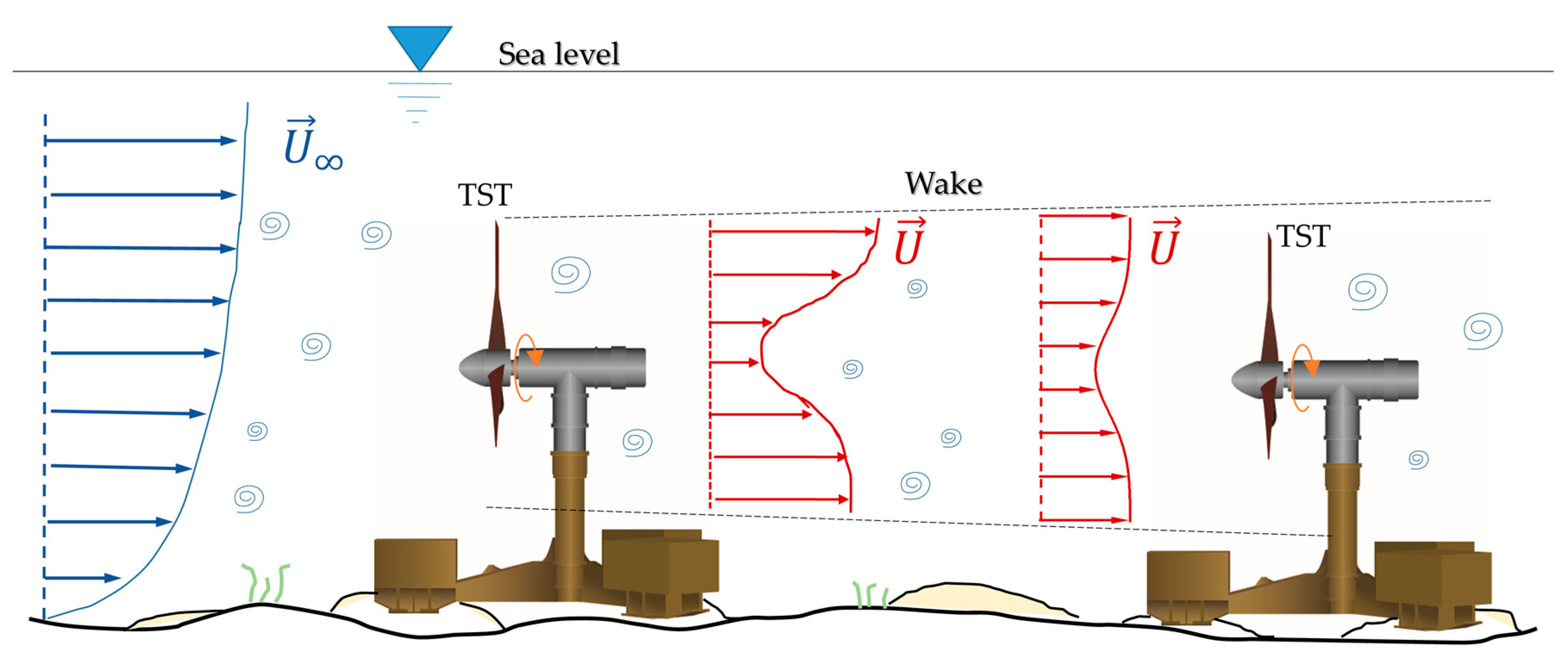Figure 1 provides the schematic lateral view of a two-row tidal stream turbine array, and highlights the key components of each turbine, namely a supporting structure laid on the seabed, a short tower supporting the nacelle, and the bladed rotor.

There are several challenges hindering the large-scale deployment of tidal stream arrays. Many of these challenges are caused by the harsh marine environment at tidal array sites, which result in significant engineering and health and safety risks associated with installing, operating and maintaining turbine foundations, turbines, and the electrical infrastructure to carry the electrical power ashore [1]. The high capital and maintenance costs of these assets are a major reason for the presently high LCOE of tidal stream energy.

Similarly to the wind energy case [2], tidal stream LCOE also depends on the energy yield of tidal turbine arrays, and this parameter can be reduced significantly due to the interactions of the wakes shed by front rows and the turbines lying in their trajectories, as in the well-known case of wind farms [3]. This issue is highlighted in the schematic of Figure 1, which also depicts the velocity profile of the wake of the turbine in the first row. When the turbines in the first and second rows are positioned coaxially, the turbine in the second row receives less kinetic energy than that in the front row, due to the velocity reduction in the wake of the latter turbine. Tidal arrays with a sufficiently large number of turbines for energy losses of this type to be observed do not exist yet, but published numerical studies indicate that the energy loss due to wake/turbine interactions may amount to about 16% of rated energy [4]. The design of tidal arrays can be a complex task, particularly when the overall blockage of the tidal channel is 2 to 5% or more of the tidal channel cross section [5], because the power harvested by a large array depletes the available kinetic energy of the current, making the resource exploitation less efficient as the number of turbines increases; for a given number of turbines, there will exist an optimal layout, i.e., definition of all turbines’ positions that maximizes the array energy yield. Therefore, as discussed in [5], tidal array design can be thought of as made of two levels, namely macro-design, whereby the total number of turbines and their gross arrangement into rows is selected, and micro-design whereby the relative positions of the turbines within a grid and the spacing between rows is optimized so as to reduce losses due to wake/turbine interactions or turbine inflow nonuniformities caused by the site bathymetry. This study focuses on the assessment and demonstration of a numerical method based on Navier-Stokes (NS) Computational Fluid Dynamics (CFD) for tidal array micro-design.

Both NS CFD and experimental studies of tidal array fluid dynamics, including the analysis of turbine/wake interactions, have been carried out in previous research. Myers and Bahaj [6] performed experiments in a flume tank using porous disks to study power extraction and wake dynamics of tidal arrays. Groups of up to three disks arranged in a front row of two disks with the third disk positioned behind them between their centers were used to analyze the effect of different lateral spacings of the two front disks on array wakes and disk thrust. These investigations found that the configuration featuring lateral spacing of 1.5 disk diameters of the front disks led to an acceleration of the flow between the front disks. In turn, this resulted in a kinetic energy up to 22% higher than the freestream value, causing the downstream disk to extract more power than the two upstream disks. In this configuration, however, the total array wake recovered more slowly than in the case of larger lateral spacing of the front disks, due to the interaction of the wakes of the front and rear disks, indicating the necessity of increasing the longitudinal spacing between the second and a possible third row with respect to that between the first and the second row. Stallard et al. [7] carried out flume tank experiments with model turbines to investigate the wake evolution with regard to velocity deficit recovery and wake lateral expansion examining several array layouts. These tests were performed with and without surface gravity wave forcing to account for the influence of marine waves and large-scale turbulence on wake dynamics, and it was found that wake recovery was not affected significantly by wave forcing. Making use of model turbine flume tank testing, Mycek et al. assessed the influence of ambient turbulence intensity on the performance and wake characteristics of a single tidal stream turbine [8], and then extended the study to the case of two aligned turbines [9], including the analysis of the impact of wake/turbine interactions on the performance and wake characteristics of the downstream turbine. Gaurier et al. [10] later extended the work of Mycek et al. to the case of a three-model turbine array with two turbines in the front row and one behind them, using a similar experimental set-up. The main objective was to analyze the performance of the rear turbine at different lateral positions with respect to the front row and for different turbulence levels. One of the findings was that the rear turbine had higher power than the front turbines when placed exactly between the two front turbines, similarly to what found in [6]. Nuernberg and Tao [11] used model turbine flume tank testing to investigate wake/turbine interactions in a four-turbine array. Their primary focus was to investigate the alterations of the wake shed by a front turbine induced by the presence of two turbines positioned symmetrically at the sides of the front turbine wake. Noble et al. [12] carried out tank testing of an array with a compact three-turbine layout similar to that considered in [10]. Using 1/15 scale instrumented model turbines configured in a symmetrically staggered layout, this study confirmed that suitably positioning one turbine in the accelerated bypass flow corridor between the wakes of two upstream turbines increased the power of the downstream turbine by up to about 10% over the power of the front turbines.

NS CFD has also been used to investigate the fluid dynamics of tidal arrays, with the key features of this technology being that it can complement the information provided by tank testing with physical data difficult or impossible to measure. NS CFD can also simulate the fluid dynamics of full-scale arrays without any constraint on the values of key nondimensional parameters such as the Froude and the Reynolds number [13]. Bai et al. [14] coupled an actuator disk model based on the blade element method theory (BEMT) to a Reynolds-averaged Navier-Stokes (RANS) code to assess the energy production of different array layouts. The method was validated using experimental data of a one-turbine experiment, and it was used to analyze staggered and rectilinear arrays. The authors found that the staggered array resulted in higher energy production, and, for this layout, they determined an optimal value of the turbine lateral spacing equal to about 2.5 rotor diameters. Malki et al. [15] used BEMT-RANS simulations to investigate the effect of turbine lateral and longitudinal spacing on wake recovery and turbine power output in the array environment. They used the BEMT-RANS method to design the layout of a 14-turbine array to maximize its energy production, and reported a 10% increase of this objective function with respect to a baseline regularly staggered array layout, achieved by optimal choice of lateral and longitudinal spacing. The effect of the array layout, with focus on the longitudinal spacing, was also investigated in [16], where turbine-resolved steady state RANS simulations were performed using the frozen rotor approach. RANS simulations in which the turbines were modeled as actuator disks were carried out by Hunter et al. [17] to determine the optimal operating conditions (tuning) of the turbines of tidal arrays with different staggered and non-staggered arrangements. Apsley et al. [18] developed an actuator line (AL) model in a RANS code, and used this approach to assess rotor/wake interaction, power and fatigue loads of two longitudinally aligned turbines and larger arrays. A variable level of agreement between available experimental data and simulations was reported. Ouro et al. [19] used a AL model and large eddy simulation CFD to assess the impact of ambient turbulence and array layout on fatigue loads and turbine performance.

The above highlights the existence of a wide range of numerical methods for the analysis and, ultimately, the design of tidal arrays. Time-dependent turbine-resolved CFD simulations are the highest-fidelity simulation-based approach to this problem, but their computational cost is also very high, due to large CFD grids required to resolve a wide range of physical scales, from those of blade boundary layers to those turbine wakes. On the other hand, BEMT-CFD simulations, in which the turbines of an array are modeled as actuator disks resolving radial flow gradients on the rotor swept area offer an adequate trade-off of computational cost and prediction quality. This is the key reason for the growing popularity of this approach, which, to the best of the authors’ knowledge, has not been validated yet against array measurements. This shortfall is one of the key outstanding issues addressed by this study. With regard to the design of tidal array layouts, it is acknowledged that positioning a turbine in the accelerated bypass flow corridor between the wakes of two adjacent front turbines may result in the power output of this downstream turbine exceeding that of the upstream turbines [6,12,14,15]. Indeed, some of these studies also performed parametric analyses to determine optimal lateral turbine spacing maximizing the bypass flow acceleration [14,15]. However, to the best of the authors’ knowledge, the expected beneficial impact of the acceleration of the bypass flow between two adjacent turbines on increasing the recovery rate of the rotor wake shed by an upstream turbine positioned on the centerline of the bypass corridor has never been assessed before. Increasing the wake recovery rate of the central wake may reduce the power loss of a turbine in the third row operating in the wake of a turbine located coaxially in the first row.

In light of the above, the objectives and the novel contributions of this work are to: (a) thoroughly validate a robust BEMT-RANS method against flume tank power and wake measurements of isolated turbines and arrays of two and four turbines featuring wake/turbine interactions, (b) use this tool to complement the physical and engineering knowledge provided by model array flume tank experiments, (c) demonstrate and estimate the potential of reducing tidal array power losses due to wake/rotor interactions by exploiting the bypass flow acceleration between neighboring turbine wakes to increase the recovery rate of an upstream central wake, and, ultimately, (d) demonstrate the potential of the adopted tool for the layout optimization of real tidal arrays accounting for bypass flow effects and wake/turbine interaction losses.

The numerical method used in this study, including the RANS code and the general turbine model are presented in Section 2. A thorough validation of the predictive capabilities of the adopted methodology is provided in Section 3. Here the one [8] and two-turbine [9] flume tank tests of Mycek et al. are simulated. Experimental data and numerical results are compared in terms of (a) turbine performance for both the single-turbine case and the two-turbine case featuring wake/turbine interactions, and (b) wake evolution, in terms of axial velocity deficit and turbulence intensity profiles. Section 4, Results, focuses on the four-turbine flume tank test reported in [11]. Here, three of the diamond-shape array layouts considered in the experiment, differing for the lateral spacing of the two turbines on either side of the wake shed by the front turbine, are simulated with the proposed method. Detailed comparisons of the measured and computed central wake are presented for further validation of the numerical method, but the simulations are then used to analyze the performance of all four turbines of the three layouts, providing data unavailable from the experiments, and enabling one to quantify the dependence of the array energy production on the wake/turbine interactions resulting by using different array layouts. Conclusions and notes on future work are provided in Section 5.

2. Numerical Method

2.1. CFD Code

The CFD code employed in this study is ANSYS^® FLUENT^® 17.2, an unstructured finite-volume Navier-Stokes code. All simulations presented below are carried out solving the RANS equations, and the effects of turbulence on the mean flow are accounted for by using Menter’s k-ω shear stress transport (SST) turbulence model [20], a RANS turbulence closure successfully tested in other recent CFD studies of tidal arrays [21,22]. The incompressible flow equations are solved using a pressure-based solution approach. The Semi-Implicit Method for Pressure Linked Equations (SIMPLE) algorithm is used to solve the momentum and pressure equations in a segregated fashion. The space discretization is second order accurate and based on an upwind flux calculation, with the variable gradients being computed with a Green-Gauss cell-based approach. Calculation of the pressure in the cell faces is based on the Pressure Staggering Option (PRESTO) scheme. Further detail on the aforementioned numerical methods can be found in the FLUENT theory guide [23].

2.2. Turbine Model

In this study, the effect of the turbine on the flow is taken into account through the use of a generalized actuator disk model embedded in the RANS code, namely the Virtual Blade Model (VBM), first conceived in the helicopter industry to simulate rotor aerodynamics [24]. VBM does not resolve the blade geometry, and models the turbine rotor as a generalized actuator disk, namely using sink terms to extract momentum from the flow, thus mimicking the interaction of a blade geometry-resolved rotor with the surrounding flow. The sink terms depend on the rotor geometry, but the requirement of resolving the flow region where these sink terms are nonzero rather than the flow region surrounding the complete rotor geometry greatly reduces grid sizes and, thus, computational cost. Although the VBM approach does not resolve circumferential gradients, it resolves radial gradients, usually providing good wake resolution a few rotor diameters downstream of the rotor under consideration. Like BEMT, VBM also combines classic lift and drag theory and the principle of conservation of linear and angular momentum. Unlike BEMT, however, the VBM approach uses all three components of the RANS momentum equations including viscous terms, rather than only a simplified one-dimensional inviscid flow momentum balance equation.

VBM simulations also require as input the number of blades, the rotor angular speed, the radial distribution of chord and twist angles of the blades, and the lift and drag curves of the blade airfoils. The sink terms embedded in the momentum equations are nonzero in a disk-shaped fluid zone representing the rotor. Their magnitude is constant at any rotor radius, and is calculated using the velocity field approaching the disk and the aforementioned blade information. More specifically, the magnitude and angle of attack (AoA) at each radius are determined, and the AoA is used to interpolate the lift and drag coefficients from the given data of the considered blade element. Blade section twist and chord, number of blades, magnitude of the relative velocity and radial width of the blade element are then used to determine the axial thrust and the torque produced by the considered annular rotor element.

The key benefit of the VBM approach for tidal array analysis and design is an optimal trade-off of computational cost and wake predicting capabilities, enabled by lower grid size requirements with respect to the case of blade-resolved simulations, and good wake predictions starting from a few rotor diameters behind the rotor. Further detail on the mathematical formulation of VBM can be found in [25].

The predictive capabilities of the FLUENT VBM approach for rotor wake and turbine performance analyses have been previously used for both horizontal axis wind turbine (HAWT) and horizontal axis tidal turbine (HATT) rotors. The method was used by Sufian et al. [26] to assess the impact of surface gravity waves on the performance of HATT rotors and the alteration of the rotor wake characteristics due to the waves. The approach was also used by Bianchini et al. [27] to assess the performance of HAWT rotors in yawed wind, study the resulting wake trajectory, and investigate the impact of wake/rotor interactions on the performance of a turbine working in the wake of an upstream rotor. The potential of the VBM approach is also shown in [28] where this method is compared with the actuator disk (AD) approach to the analysis of wind turbine wakes.

3. Validation

In order to validate the VBM approach for HATT array applications, the one- and two-turbine experiments carried out in the IFREMER flume tank and reported by Mycek et al. [8,9] are considered. The flume tank has a length of 18 m, and a rectangular cross section of width b = 4 m and depth h = 2 m, and the reported experiments employed 1/30th scaled HATTs. Each rotor was connected to a supporting structure above the free surface by means of a supporting tower, and was equipped with a torque sensor. The hydrodynamic thrust was measured by a load cell on the supporting structure to which the tower was connected. The main geometric data of the tested rotors are reported in

Table 1. Main geometric data of turbine rotors of the IFREMER flume tank tests [8,9].

Turbine Element	Geometry INFO
Hydrofoil	NACA 63418
Rotor radius (D/2)	350 mm
Hub radius	46 mm
Hub length	720 mm

, whereas the radial profiles of blade chord and twist are reported in [8].

The flume tank is designed to allow a freestream velocity between 0.1 and 2.2 m/s. Different levels of environmental turbulence intensity are achieved by inserting honeycomb grids with different refinements before the testing section of the tank. The experiments aim at characterizing the turbine performance in terms of power coefficient $C_P$ and thrust coefficient $C_T$, whose definitions are provided by Equations (1) and (2), respectively:

$$C_P=\frac{P}{\frac{1}{2}\rho \pi {\left(\frac{D}{2}\right)}^2{U}_{\infty }^3},$$

(1)

$$C_T=\frac{T}{\frac{1}{2}\rho \pi {\left(\frac{D}{2}\right)}^2{U}_{\infty }^2},$$

(2)

where the symbols $P$, $T$, $U_{\infty }$ and $D$ denote, respectively, rotor power, overall thrust on rotor and supporting structure, freestream velocity, and rotor diameter. Flow velocity data were acquired through Laser Doppler Velocimetry. In [8] one isolated turbine was considered, whereas in [9] an array of two turbines aligned along the direction of the freestream (tandem configuration) was considered. In the latter study, the performance and the wake of the downstream turbine were measured, with longitudinal distance of the downstream turbine from the front turbine varying between 2D and 12D. The performance of the downstream turbine was evaluated by changing its rotor angular speed ω while keeping constant the freestream velocity $U_{\infty }$ upstream of the front turbine. This choice results in the tip speed ratio (TSR) λ of the downstream turbine, defined by

$$\lambda =\frac{\omega D}{2U_{\infty }},$$

(3)

varying linearly with $\omega$. Both the one- and two-turbine experiments provided an extensive characterization of the wake in terms of its velocity and turbulence intensity profiles behind both turbines, as shown below.

3.1. Physical Domain and CFD Set-Up

The selected physical domain has the same cross-section of the IFREMER flume tank, and this implies that the blockage ratio (BR) of the experiments and the simulations is also the same. Here, BR is defined as the ratio between the rotor swept area and the tank cross section, and is given by:

$$BR=\frac{\pi D^2}{4bh}100,$$

(4)

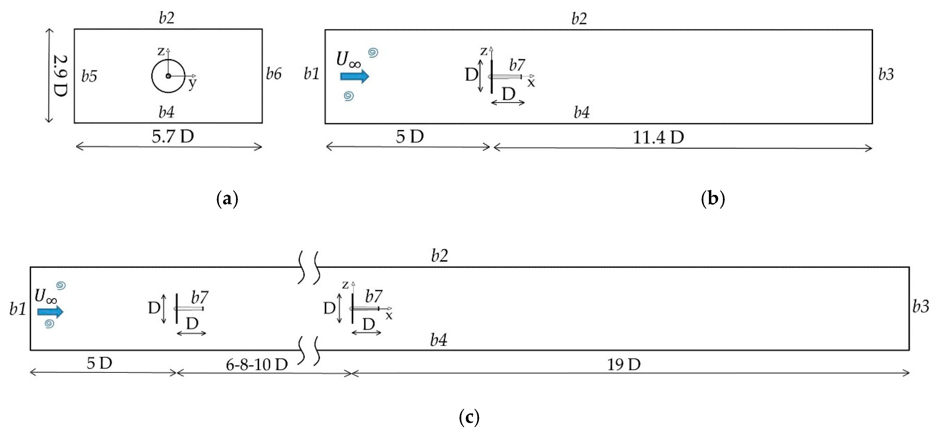
Inserting the geometric data of the tank and the rotor sections into Equation (4) yields a relatively small BR value of about 4.8%. The upstream and downstream lengths of the modeled tank were increased to minimize the detrimental impact of spurious reflections from the far field boundaries on the computed solutions. Figure 2 presents a schematic of the modeled physical domain and indicates the boundary conditions (BCs) imposed on the boundaries of the considered domain. The specific condition types applied on each boundary are reported in

Table 2. Boundary conditions on boundaries of physical domains of Figure 2.

Label	BC Type
Velocity inlet	b1
Inviscid wall	b2, b7
Pressure outlet	b3
Viscous wall	b4, b5, b6

.

A velocity inlet BC was applied at the inlet of the numerical tank (boundary b1). Here, a freestream velocity $U_{\infty }=$ 0.8 m/s, a turbulence intensity $I_{\infty }=3\%$, and a turbulence length scale l = D/2 were enforced. The freestream values of the turbulence kinetic energy $k_{\infty }$ and the specific dissipation rate ${\omega }_{\infty }$ variables at the inlet boundary are:

$$k_{\infty }=\frac{3}{2}{\left(U_{\infty }{I}_{\infty }\right)}^2,$$

(5)

$${\omega }_{\infty }=\frac{k_{\infty }^{0.5}}{C_{\mu }^{0.25}l},$$

(6)

It was observed that the level of turbulent kinetic energy (TKE) k along the tank varied along the tank with respect to the specified value of $k_{\infty }$, and this variability was found to be quite sensitive to the value of ${\omega }_{\infty }$. The choice $l=D/2$ was made after a parametric study aiming to minimize the variation of turbulence intensity with respect to the value of 3% measured in the experiment and enforced at the inlet boundary of the simulations reported in this section. Blackmore et al. [29] also investigated the impact of the value of l enforced at the inlet boundary on the k flow field in a flume tank with and without porous disks. Making use of RANS simulations with and without actuator disk and experimental data for validation, they determined optimal values of l, and modified the source terms of the k-ε turbulence model to maximize the agreement of numerical results and experimental data.

A pressure outlet BC was applied at the outlet of the tank (boundary b3), where a zero differential pressure was enforced. Viscous wall BCs were used on the flume bed and lateral wall, whereas a rigid lid (inviscid wall) BC was used at the free surface boundary.

3.2. Mesh Refinement Analysis

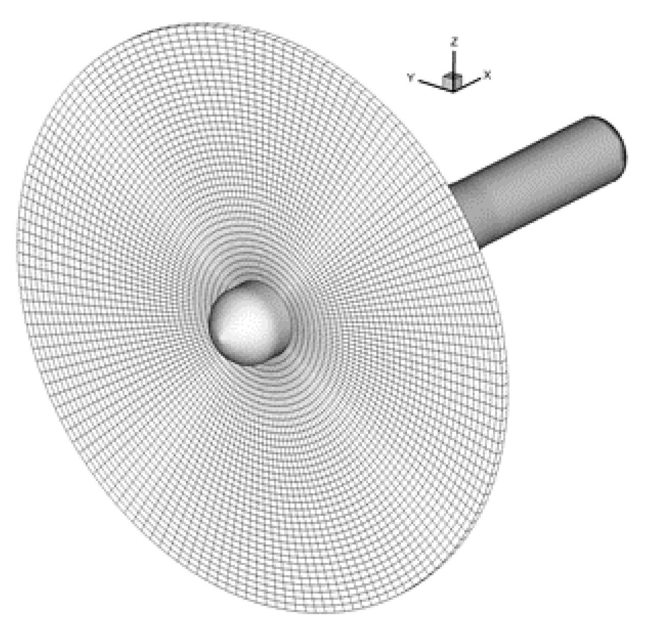
The turbine model used in the simulation of the IFREMER tests is reported in Figure 3. The model includes the rotor nacelle, on the surface of which an inviscid wall BC was applied. The model does not include the tower connecting the nacelle to the supporting structure above the free surface. This choice was made to prevent the flow unsteadiness resulting from vortex shedding behind the cylindrical tower, which would have required the use of time-dependent simulations, increasing significantly the computational burden of all analyses. The lift and drag curves of the NACA63418 airfoil were computed with the XFoil panel code [30]. The Reynolds number Re_c based on the local chord and the estimated relative velocity along the blade for a TSR range between 2 and 7 varied between $7.00\times {10}^4$ and $1.85\times {10}^5$ in the XFoil analyses.

To determine the level of spatial refinement required to achieve grid independence of the CFD solutions, four grid levels have been used for the analysis of the one-turbine flume tank configuration. All meshes consist of tetrahedral elements and have been generated with the mesh tool ANSYS MESHING. The four meshes differ primarily for (a) the number of rotor elements $N_R$, controlled by changing the maximum rotor element size ${\Delta }_R$, and (b) the number of elements in the wake region, controlled by changing the maximum element size ${\Delta }_w$ in the wake region, which has axial length 10D. The remaining part of the computational domain has comparable element sizes and numbers in all four grids. An inflation layer is used on both the flume bed and lateral walls, and the distance of the first node layer from these boundaries is such that the maximum nondimensionalized minimum wall distance y⁺ is about 1 in all cases.

Table 3. Main parameters of four grids used for mesh refinement analysis.

Mesh	${\mathit{N}}_{\mathit{R}}$	${\mathit{\Delta }}_{\mathit{R}}$	${\mathit{N}}_{\mathit{W}}$	${\mathit{\Delta }}_{\mathit{W}}$	${\mathit{N}}_{\mathit{E}}$
M1	1660	0.0043	633,329	0.028	5,378,374
M2	5328	0.003	2,010,165	0.02	10,186,971
M3	13,509	0.0016	3,598,772	0.015	17,464,945
M4	13,509	0.0016	8,637,895	0.011	24,838,752

, in which M1 denotes the coarsest grid and M4 the finest one, provides the main parameters of all four grids, including the total number of elements $N_E$.

Table 4. Power coefficient C_P and thrust coefficient C_T computed with grids M1 to M4.

Mesh	${\mathit{C}}_{\mathit{P}}$	${\mathit{C}}_{\mathit{T}}$
M1	0.46	0.79
M2	0.442	0.78
M3	0.445	0.785
M4	0.447	0.786

reports the values of the power coefficient $C_P$ defined by Equation (1), and the thrust coefficient $C_T$ defined by Equation (2), determined by using the four aforementioned grids for the analysis of the isolated turbine configuration. The data refer to the design TSR λ of 3.67. One notes that both the $C_P$ and the $C_T$ estimates computed on grids M2 differ by less than 1% from their M3 counterparts, indicating that the level of spatial refinement of grid M2 is adequate for reliably estimating turbine performance parameters.

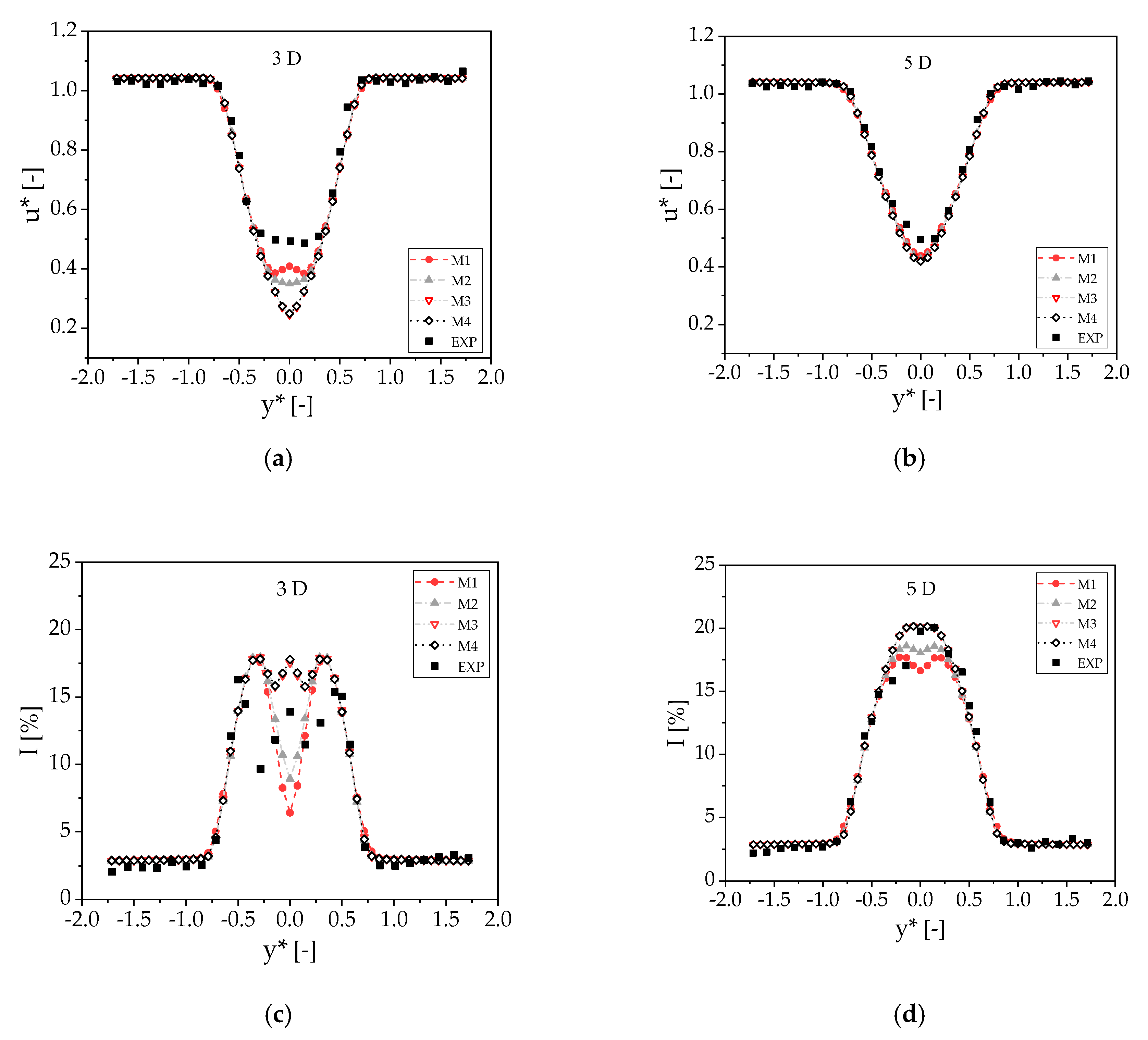
The sensitivity of the wake resolution to the mesh refinement is assessed in the four subplots of Figure 4, which all refer to the design TSR λ = 3.67. The profiles of the nondimensionalized axial velocity profiles u* on a horizontal line through the rotor axis at distance 3D and 5D from the rotor center computed with the four grids are provided in Figure 4a,b respectively. The velocity u* is given by:

$$u^{*}=\frac{u}{U_{\infty }},$$

(7)

where u is the local axial velocity component. The variable y* on the x-axis is the distance from the rotor center nondimensionalized by D. The measured profiles are also reported in both figures. At the distance of 3D, the M3 profile provides a grid-independent solution, whereas further downstream, at the distance of 5D, all four profiles are in quite good agreement. Very good agreement between measured and computed velocity profiles is also observed. The comparison of the computed and measured profiles of local turbulence intensity I on the same transversal lines at 3D and 5D is presented in Figure 4c,d respectively. The local turbulence intensity I is linked to the local TKE k by Equation (5), which defines this relation at the inflow boundary. As in the case of the velocity profiles, a grid-independent solution is achieved using grid M3, and, overall, good agreement of computed and measured data is noted. The agreement between simulations and experiments improves moving downstream of the rotor. This is because wake mixing increases and circumferential nonuniformities decrease, resulting in the wake pattern becoming closer to the assumption of circumferential uniformity of the BEMT module of the VBM approach. It is also noted that the differences between the velocity and turbulence intensity profiles determined with the M2 and M3 simulations are localized in a relatively small circular region around the rotor axis, and, for this reason, the use of the M2 grid settings in a multi-turbine simulation rather than those of grid M3, is unlikely to result in significant errors affecting turbine power estimates, also in the presence of rotor/wake interactions. That the grid resolution required for a fully grid independent estimate of the rotor performance, grid M2 in the present case, is lower than that required for a fully mesh-independent wake resolution, is regularly observed in CFD simulations of turbines and their wakes [31].

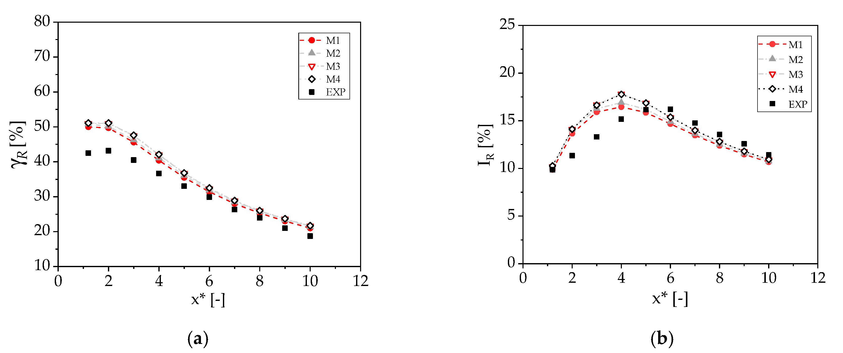
The area-averaged velocity deficit ${\gamma }_R$ along the tank length measured behind the rotor is compared with the same variable determined with the simulations using grids M1 to M4 in Figure 5a. The velocity deficit γ at a point in the rotor wake is defined as:

$$\gamma =100\left(1-\frac{u}{U_{\infty }}\right),$$

(8)

The area-averaged velocity deficit ${\gamma }_R$ is defined as:

$${\gamma }_R\left(x\right)=\frac{{\iint }_A\gamma \left(x,y,z\right)dydz}{{\iint }_{A}dydz},$$

(9)

where $A$ denotes the rotor swept area. The use of the swept rotor area rather than the axial position-dependent greater wake cross sectional area in the calculation of ${\gamma }_R$ leads to slightly different results with respect to the case in which the actual wake cross section is used. However, the definition based on the rotor swept area was adopted because the measured variable is based on this choice. The variable x* along the horizontal axis of Figure 5a is the position x along the flume tank length nondimensionalized by D. One notes that the M3 ${\gamma }_R$ profile is grid-independent over the entire considered length and that the differences between the coarser M2 profile and the M3 profile decrease moving away from the rotor, and are fairly small already at 6D behind the rotor. A similar comparison is considered in Figure 5b for the area-averaged turbulence intensity $I_R$, whose definition is structurally similar to that of the velocity deficit provided by Equation (9). Also in this case, a fully grid-independent solution is obtained with grid M3. It is also noted that all CFD simulations overpredict significantly the turbulence production in the near wake region, whereas the agreement between simulations and measured data becomes excellent from between 5D and 6D. The overprediction of turbulence behind the rotor is believed to be caused by the lack of a blade-resolved model, a feature which does not hinder significantly this study, as neither here nor in full-scale arrays are adjacent rotors likely to be placed at a longitudinal distance of less than 5D.

3.3. Performance and Far-Wake Analysis of Isolated Rotor

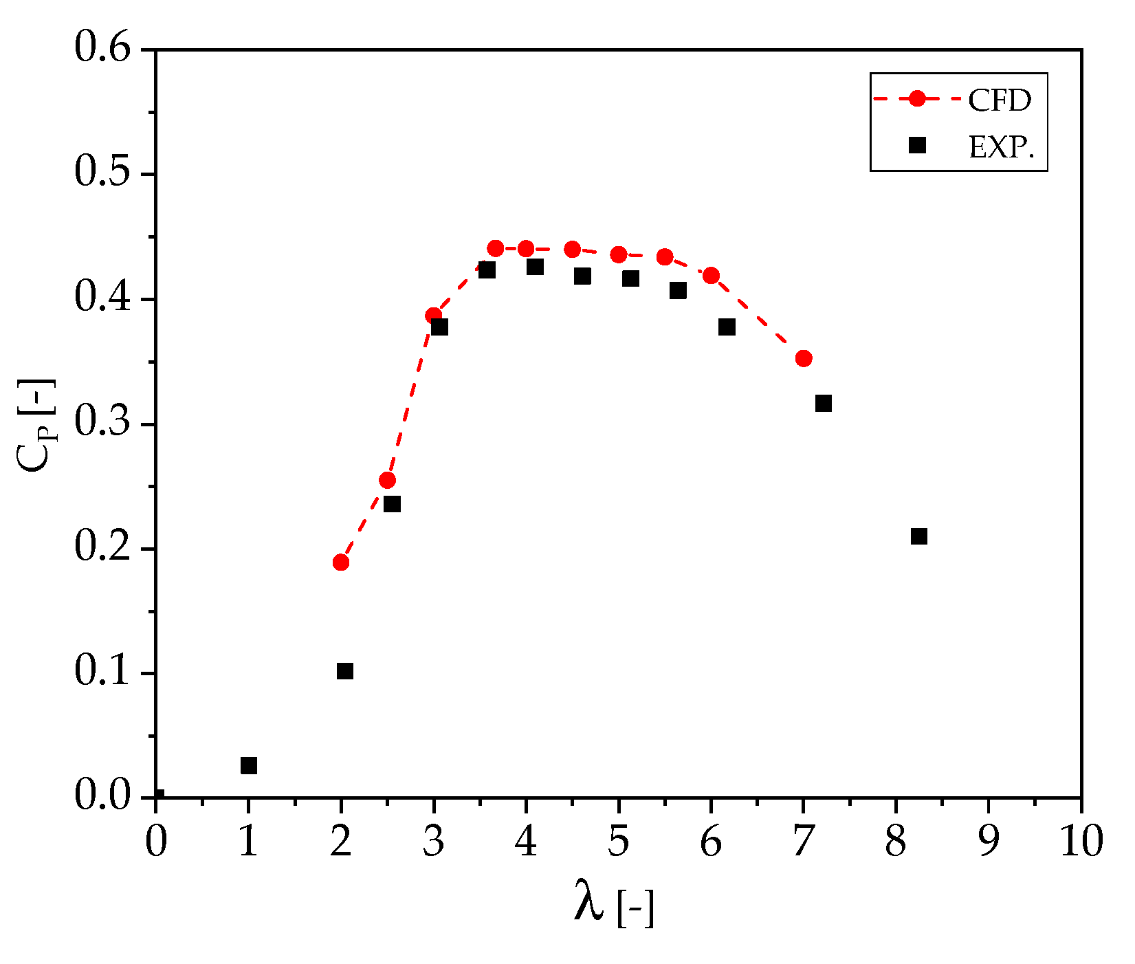
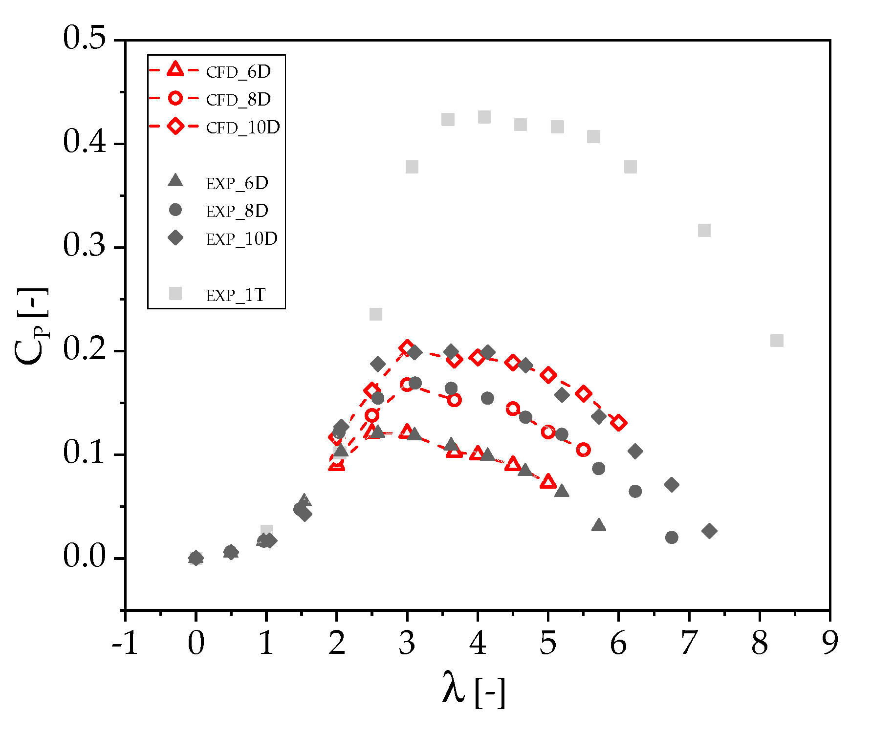
Here the isolated turbine flume tank experiment of [8] is examined in further detail using the grid M3, which has been shown to produce grid-independent results. Figure 6 compares the measured and computed power coefficient $C_P$ defined by Equation (1) over a wide range of TSR values, before and after the design value $\lambda$ = 3.67. An overall very good agreement of measured and computed $C_P$ profiles is observed. For TSR between 3 and 6, the maximum, minimum and mean percentage difference between the CFD and experimental $C_P$ estimates are 8.9%, 3.4% and 5.2%, respectively. At design conditions, CFD overestimates the measured power coefficient by only about 3.5%.

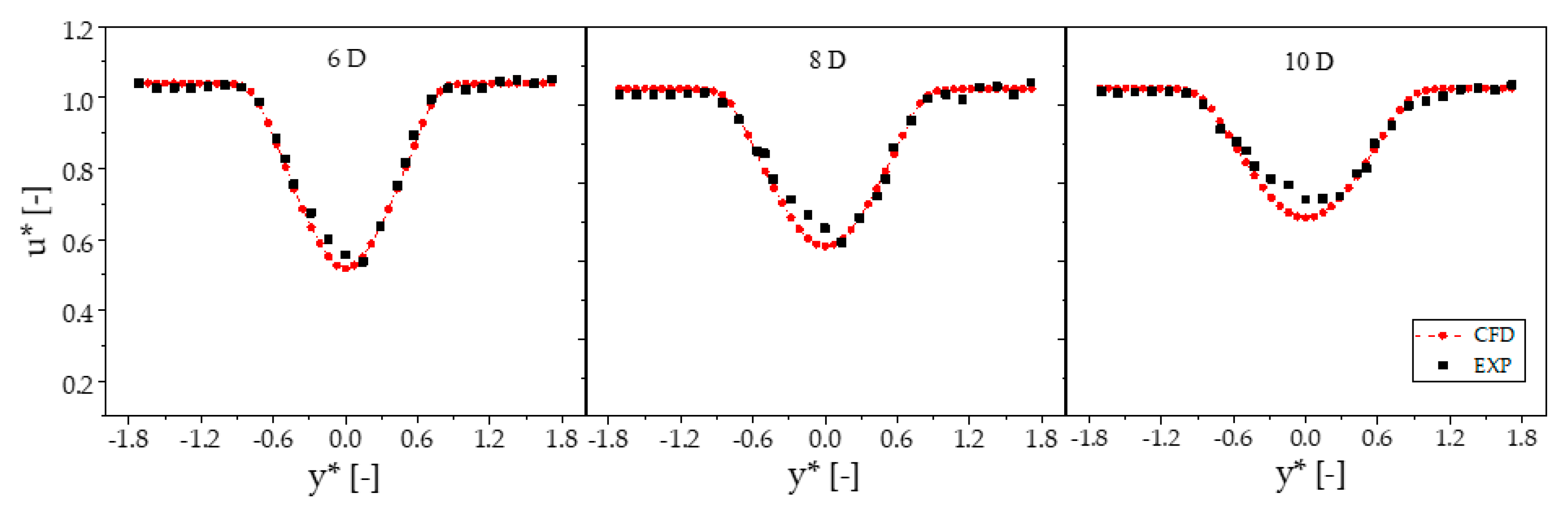
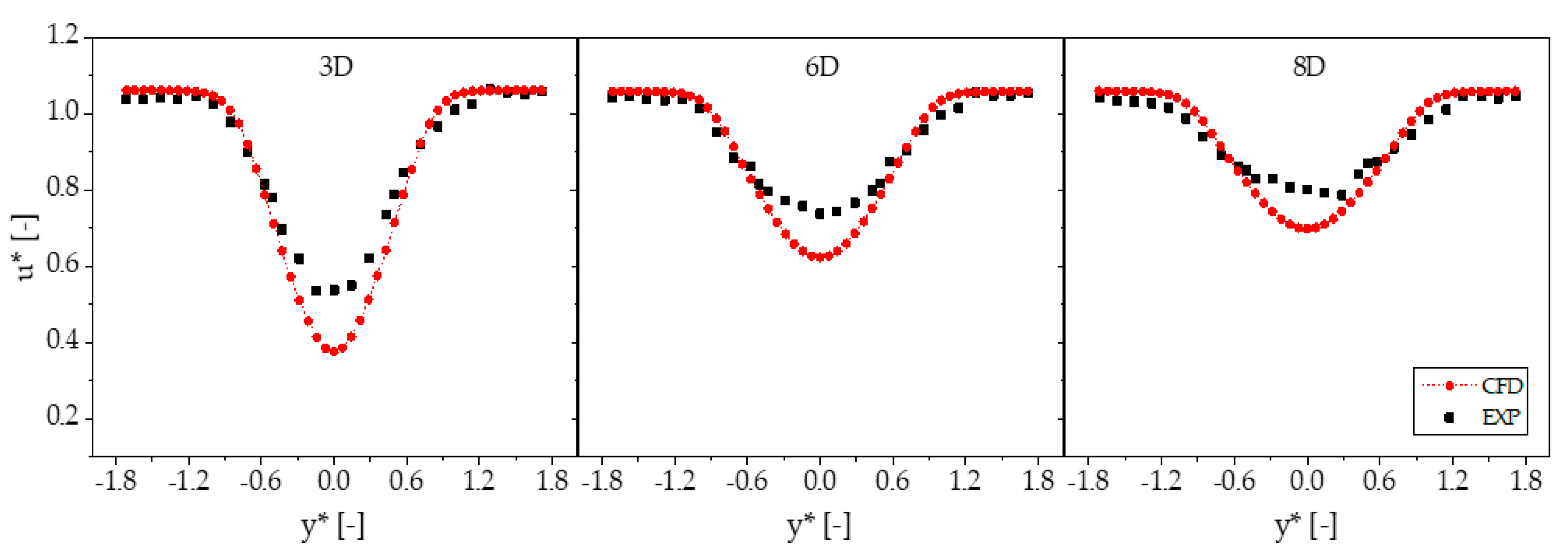
Figure 7 presents the evolution of the wake in terms of nondimensionalized velocity u* on a horizontal line at rotor hub height at 6D (left subplot), 8D (mid subplot), and 10D (right subplot) downstream of the rotor. It is seen that the CFD simulation captures very well the wake evolution. The differences between computed and measured u* profiles at 6D, 8D and 10D, expressed as root mean square (RMS) values of the difference between measured and computed data, are 0.019, 0.023 and 0.024, respectively. The low-velocity circular area expands notably between 6D and 10D, and, as this happens, the velocity deficit on the wake centerline decreases notably, from 48.3% at 6D to 29% at 10D. All these phenomena are well captured by the considered VBM method. This provides initial evidence of the capability of this approach to resolve far-wake physics, a capability required for analyzing wake/turbine interaction losses in tidal arrays. 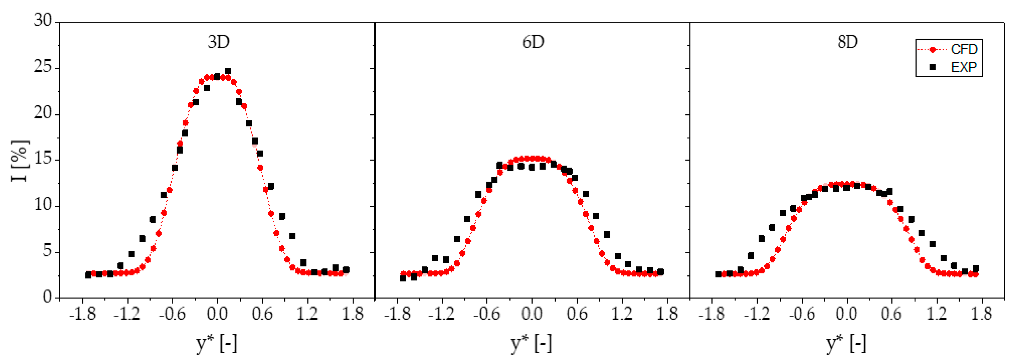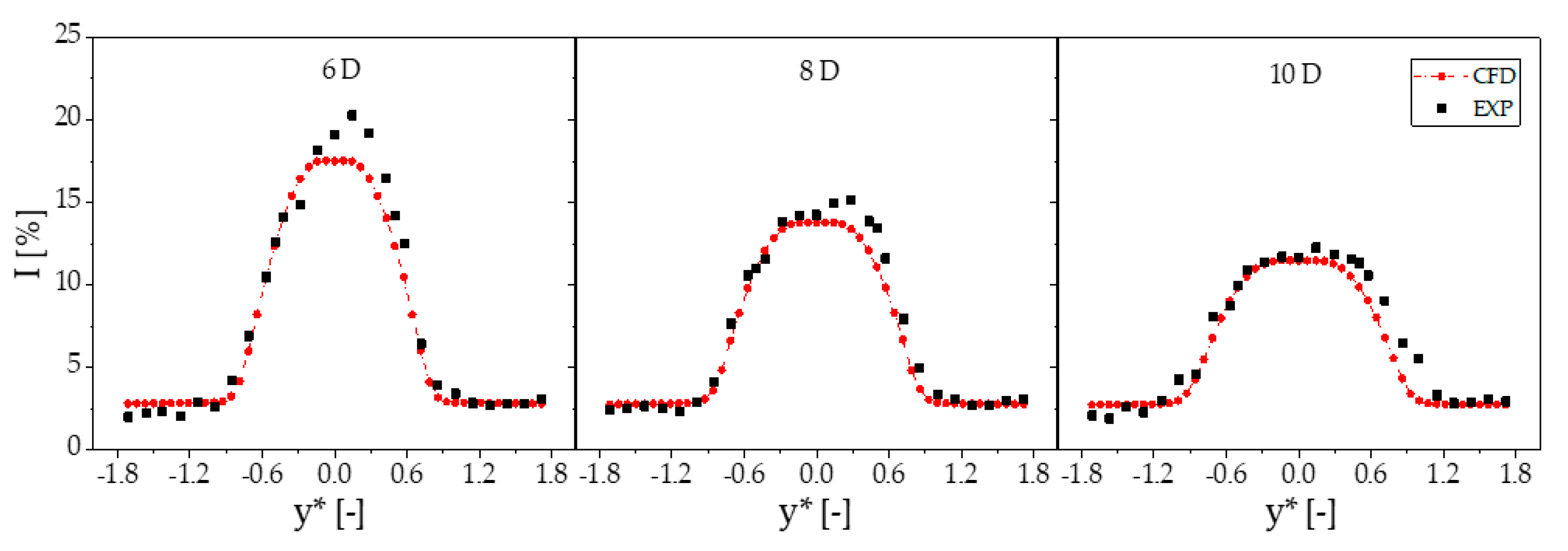The transverse profiles of computed and measured turbulence intensity I at the same positions considered for the wake velocity analysis of Figure 7 are compared in Figure 8. An overall very good agreement between measured data and numerical results is observed again. The differences between computed and measured I profiles at 6D, 8D and 10D, expressed as RMS values of the difference between measured and computed data, are 1.2%, 0.9% and 1.0%, respectively. Like in the case of the velocity, one sees that also the region of high TKE associated with the wake widens downstream of the rotor, and its central peak decreases due to diffusion. The adopted CFD approach captures very well these physical phenomena. The numerical profiles of Figure 8 also demonstrate how the choice made for the turbulence length scale yielding the value of the freestream specific dissipation rate ${\omega }_{\infty }$ defined by Equation (6) succeeds at maintaining the prescribed ambient turbulence intensity of 3% outside the wake throughout the entire physical domain. Indeed, this is also evident in the turbulence intensity plots of Figure 4c,d.

3.4. Performance and Wake Analysis of Two Longitudinally Aligned Rotors

The VBM method has been validated also for a two-turbine set-up involving wake/rotor interactions using the experimental data provided in [9]. In this flume tank experiment, two identical model turbines, whose geometry is provided in [8] and summarized in Table 1, are positioned in a coaxial set-up with the water flow being parallel to the machine axes, as indicated in the schematic of Figure 2c. This configuration results in the downstream turbine operating in the wake of the front turbine. The boundary conditions for these two-turbine simulations are also indicated in Figure 2c and Table 2. The simulations presented below refer to the conditions of the subset of experimental tests featuring freestream velocity $U_{\infty }$ = 0.8 m/s and ambient turbulence intensity $I_{\infty }=3\%$. Three experiments differing for the longitudinal distance of the two turbines, set at 6D, 8D and 10D, are considered. As in the flume tank experiments, in the VBM simulations the upstream turbine is kept at constant angular speed of 9.14 rad/s corresponding to the design TSR value of 4 whereas the TSR of the downstream turbine is varied by changing its angular speed. The CFD grid of the two-turbine simulations was generated adopting the key parameters of the mesh M3 used in the mesh refinement analysis of the single-turbine case.

Figure 9 compares measured and computed power curves of the downstream turbine for all three considered values of its longitudinal distance from the upstream turbine. The power coefficient reported along the vertical axis is obtained by nondimensionalizing the turbine power with a reference power based on the freestream velocity $U_{\infty }$ = 0.8 m/s upstream of the front turbine. Even though the TSR of the front turbine is fixed throughout all the two-turbine experiments discussed below, Figure 9 also reports the measured power curve of the front turbine for reference. An excellent agreement between the measured power curve of the downstream turbine and the power curve computed with the VBM approach is observed for all three longitudinal spacings. This demonstrates the VBM capability of adequately accounting for wake/rotor interactions on turbine power output, and, thus, assessing the performance of tidal arrays. It is also noted that, for the considered level of ambient turbulence, decreasing the longitudinal turbine spacing from 10D to 6D results in nearly halving the power of the downstream turbine due to the velocity deficit associated with the wake of the front rotor becoming larger. Furthermore, the power of the downstream turbine is about half that of the front turbine even for a longitudinal spacing of 10D, indicating that even at such fairly large distance, the velocity deficit of the front turbine wake is still significant.

The measured and computed wake velocity profiles at 3D, 6D and 8D behind the downstream turbine for the case in which the downstream turbine is at 8D from the front turbine are compared in Figure 10. Although the qualitative agreement between measured and computed profiles is good, the differences between the two profiles are more pronounced than those in the wake of the front turbine, as visible in Figure 7. One possible reason for this discrepancy is a lack of coaxial alignment of the upstream wake centerline and the downstream turbine rotor axis. One possible reason for this misalignment may be blockage effects due to the rotor supporting structure. The measured and computed turbulence intensity profiles at 3D, 6D and 8D behind the downstream turbine for the case in which the downstream turbine is at 8D from the front turbine are compared in Figure 11. Quite interestingly, the agreement of these profiles is notably better that that observed for the velocity profiles in Figure 10. The reason for the different level of agreement between measurements and simulations for the wake velocity and turbulence intensity profiles is presently being investigated, and one possible reason is the need for small alterations of the VBM model to improve its predictions in the case of rotors working at high levels of ambient turbulence [29].

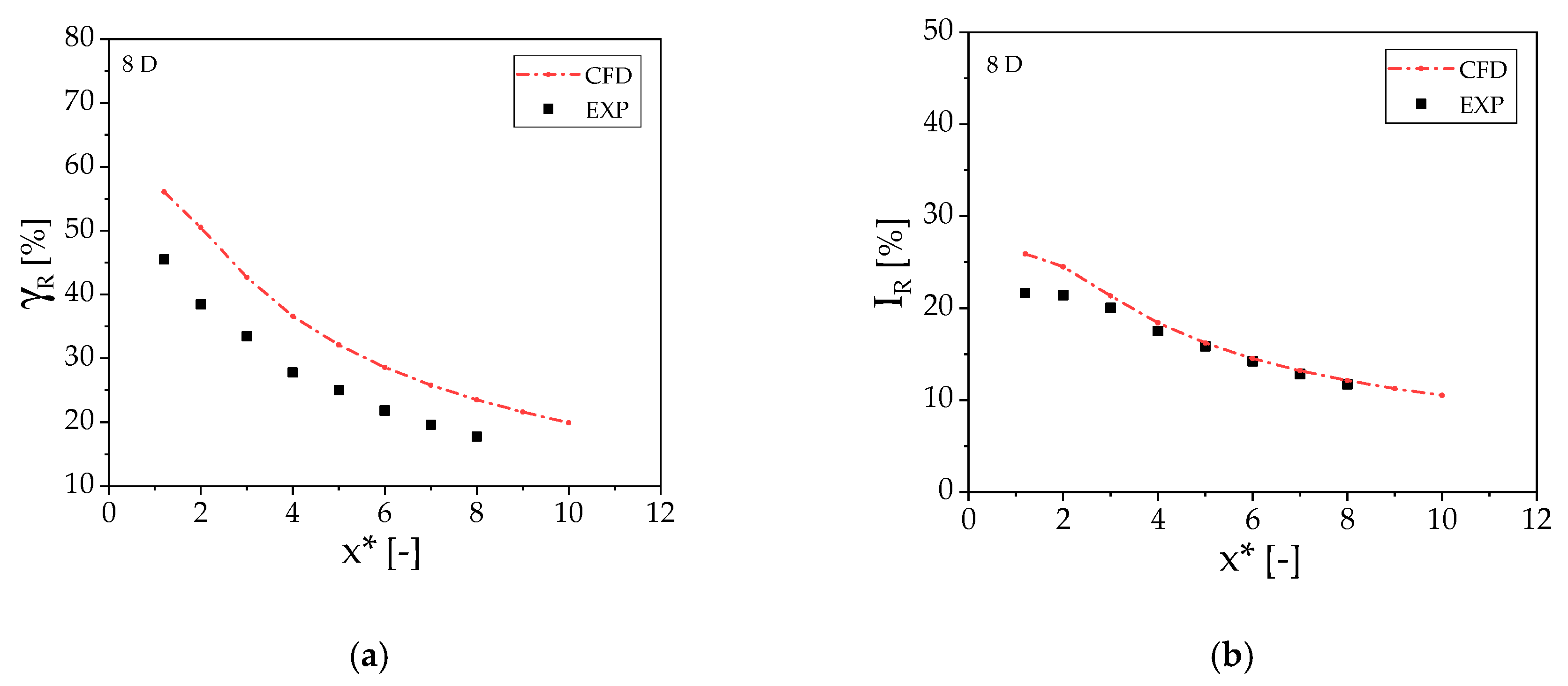
The longitudinal profiles of the area-averaged wake velocity deficit ${\gamma }_R$ and the turbulence intensity $I_R$ behind the downstream rotor are depicted in Figure 12a,b respectively. Both plots confirm the conclusions made on the basis of the comparisons in Figure 10 and Figure 11, namely an overprediction of the wave velocity deficit and an excellent prediction of the wake turbulence intensity, particularly from 3D behind the rotor.

4. Results

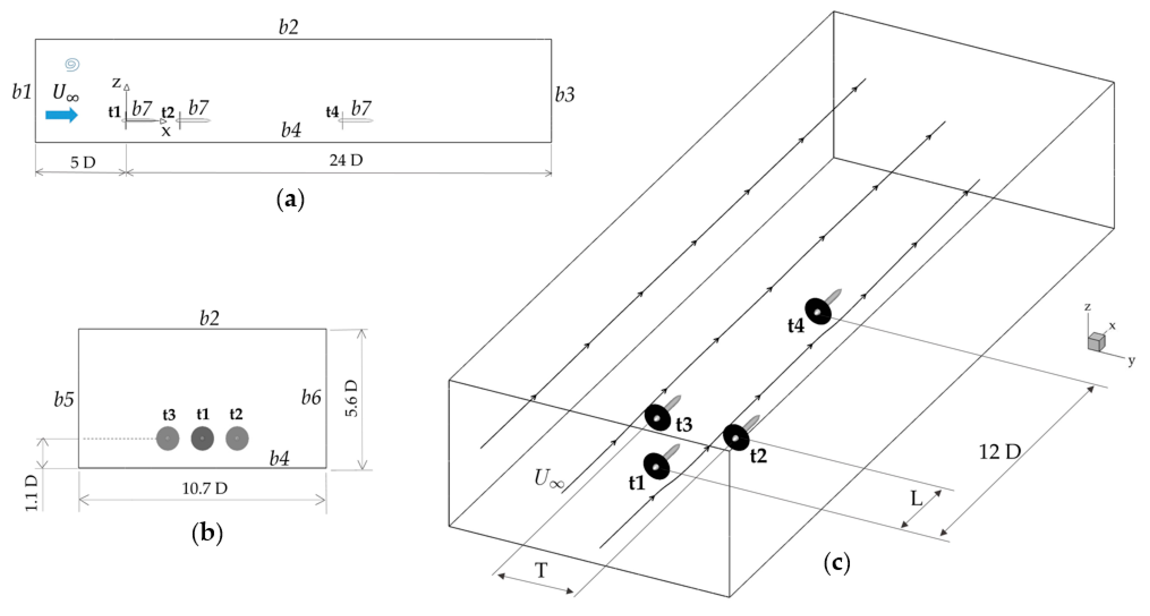
To demonstrate the strengths of the VBM approach for the analysis and design of tidal turbine arrays, a four-turbine array module with general layout of the type depicted in Figure 13 is considered. The key objectives of the analyses below are (a) assessing the sensitivity of the power of the downstream turbine t4 to the transverse spacing T of turbines t2 and t3, and (b) determining the value of this parameter maximizing the power capture of the array. In light of possible beneficial impact of the accelerated bypass flow between turbines t2 and t3 on the characteristics of the wake of the front turbine t1, the key aim is to determine if there exist values of T that maximize the recovery rate of the wake shed by the upstream turbine t1, thus increasing the onset water speed of turbine t4.

The analyses below have as the starting point the flume tank experiments of Nuernberg and Tao [11], who investigated turbine/wake interactions of this array layout. Those experiments were carried out in the circulating water channel at Shanghai Jiao Tong University (SJTU). The 8 m-long test section of the flume has rectangular cross section with width of 3 m and depth of 1.6 m. The facility allows for current velocity between 0.25 and 0.8 m/s, and operates with ambient turbulence intensity of 2%. The 1/70th scaled three-blade model turbines, representative of turbines with rotors of up to 20 m diameter, are bottom mounted through a supporting structure with an elliptical cross section. The main geometric data of the model turbines are provided in

Table 5. Main geometric data of turbine rotors of the SJTU flume tank tests [8,9].

Label	BC Type
Hydrofoil	NREL S814
Rotor radius	140 mm
Hub radius	30 mm
Hub length	558 mm

. The bottom plate of the supporting structure of the lateral turbines t2 and t3 is attached to a supporting frame on the flume bed. This method enables varying both the transverse spacing T (twice the distance of each lateral turbine from the centerline joining turbines t1 and t4) and the longitudinal spacing L (distance of turbines t2 and t3 from turbine t1 along the water stream direction) of turbines t2 and t3, obtaining different array layouts. The freestream water speed is 0.52 m/s, and the rotational speed of turbines t1, t2 and t3 is kept to 14.86 rad/s in all tests, resulting in these three turbines working at the design TSR value λ = 4. In the experiments, two values of L were considered, namely 3 and 5 rotor diameters, but only the data for L = 3D are considered in the analysis below; this longitudinal set-up is denoted by L3. For both values of L, three arrays with T equal to 1.5D, 2D and 3D were tested in the experiments; these set-ups are denoted by T1.5, T2 and T3. The rear turbine t4 was kept at 12D from the front turbine t1 in all layouts. The instantaneous velocity field in the symmetry plane of the arrays is measured by means of particle image velocimetry. The wake is characterized in terms of velocity deficit γ and turbulence intensity I on the centerline of turbines t1 and t4. The M3 grid settings provided in Table 3 have been used for the grids to simulate the SJTU experiments. Figure 13 depicts the physical domain of the simulations and, using the same symbols defined in Table 2, also illustrates the imposed boundary conditions. All VBM simulations have been performed imposing $U_{\infty }=$ 0.52 m/s and ω = 14.86 rad/s, and using airfoil lift and drag curves computed for $R{e}_c=7\times {10}^4$. The supporting structure, the bottom plate and the supporting frame have not been included in the turbine model to reduce grid sizes and computational costs. Preliminary analyses have shown that the inclusion of the tower towers does not alter significantly the results obtained without these geometric elements.

4.1. Comparison of Measured and CFD Data

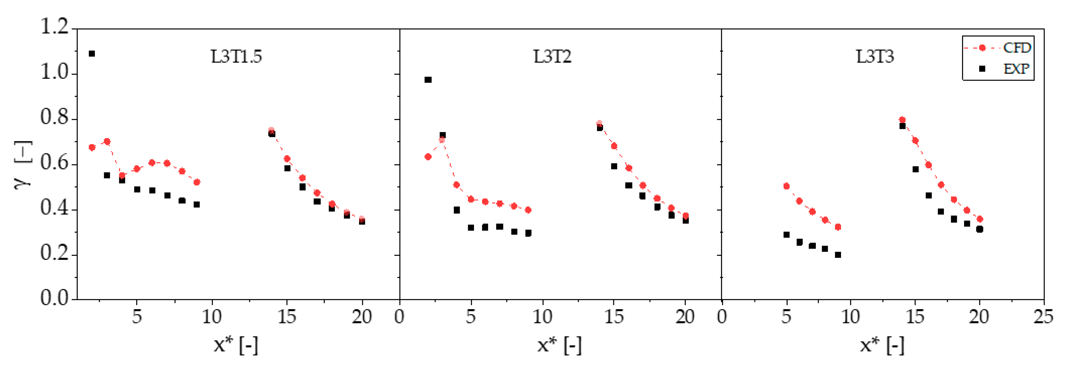
In the SJTU experiments, the velocity field on the array symmetry plane was measured between 2 and 9 diameters downstream of turbine t1, and also between 14 to 20 diameters downstream of turbine t1. 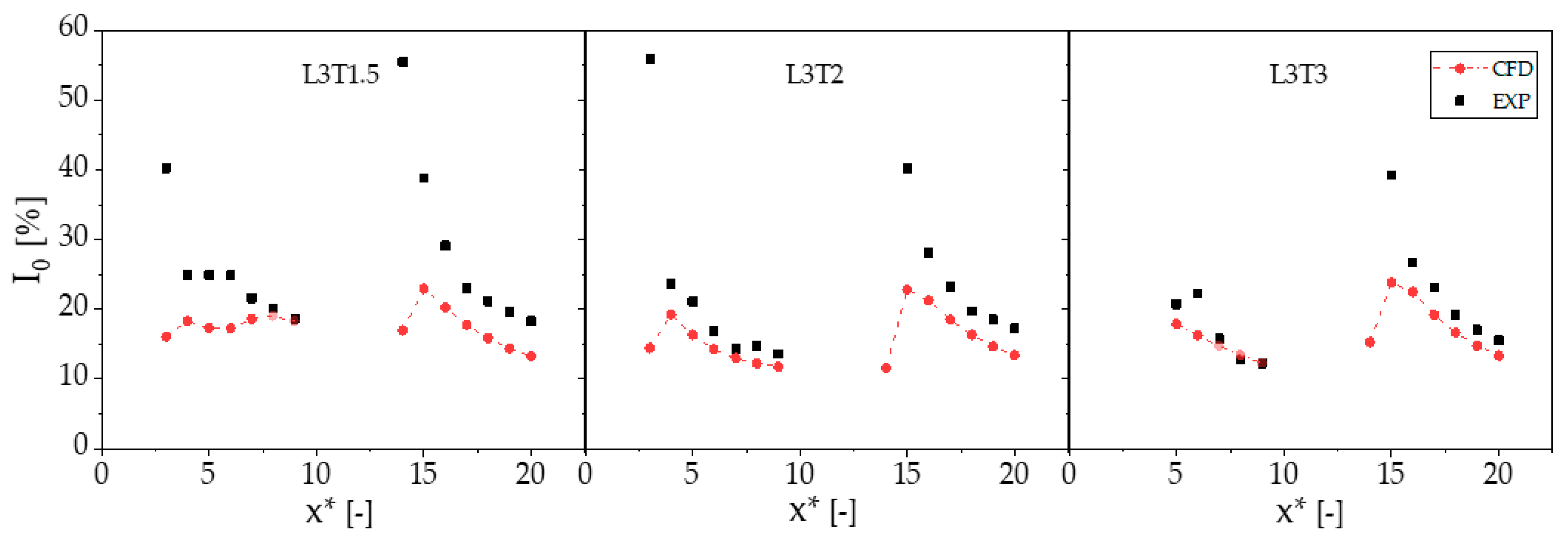The three subplots of Figure 14 compare the measured and computed profiles of velocity deficit γ on the centerline of rotor t1 and t4 for the arrays with L = 3D and transverse spacing T of 1.5D, 2D and 3D, whereas the three subplots of Figure 15 compare the measured and computed profiles of turbulence intensity I on the same centerline. The subplots of Figure 14 highlight fair agreement between experiments and simulations. Both result sets predict a sharp increment of γ at x* = 14D with respect to the value at x* = 10D, which is due to a velocity reduction across turbine t4 positioned at x* = 12D. Measurements and simulations also present comparable velocity gradients on the same centerline except for the region between 0 and 3D. The position x* = 3D is where the two lateral turbines are placed, and their wakes start interacting with that of the front turbine. The measured and computed levels of the γ profiles present some discrepancies, particularly downstream of the front turbine t1. It is noted, however, that the profiles in Figure 14 refer to the rotor centerline. The differences between measured and computed velocity deficit has been found to be maximum in the analysis of the IFREMER test case, as visible in Figure 7, whereas the agreement between the area-averaged values has been found to be significantly higher, as visible in Figure 5. Unfortunately, area-averaged values are not available for the SJTU experiments, but the conclusions drawn from the analysis of the IFREMER tests supports the assumption that the discrepancies between measured and computed γ profiles in Figure 14 are unlikely to have a significant impact on the analysis of the array energy yield. The measured and computed profiles of I in Figure 15 also show a fair level of qualitative agreement. The type of discrepancy is consistent with that observed for the velocity deficit profiles.

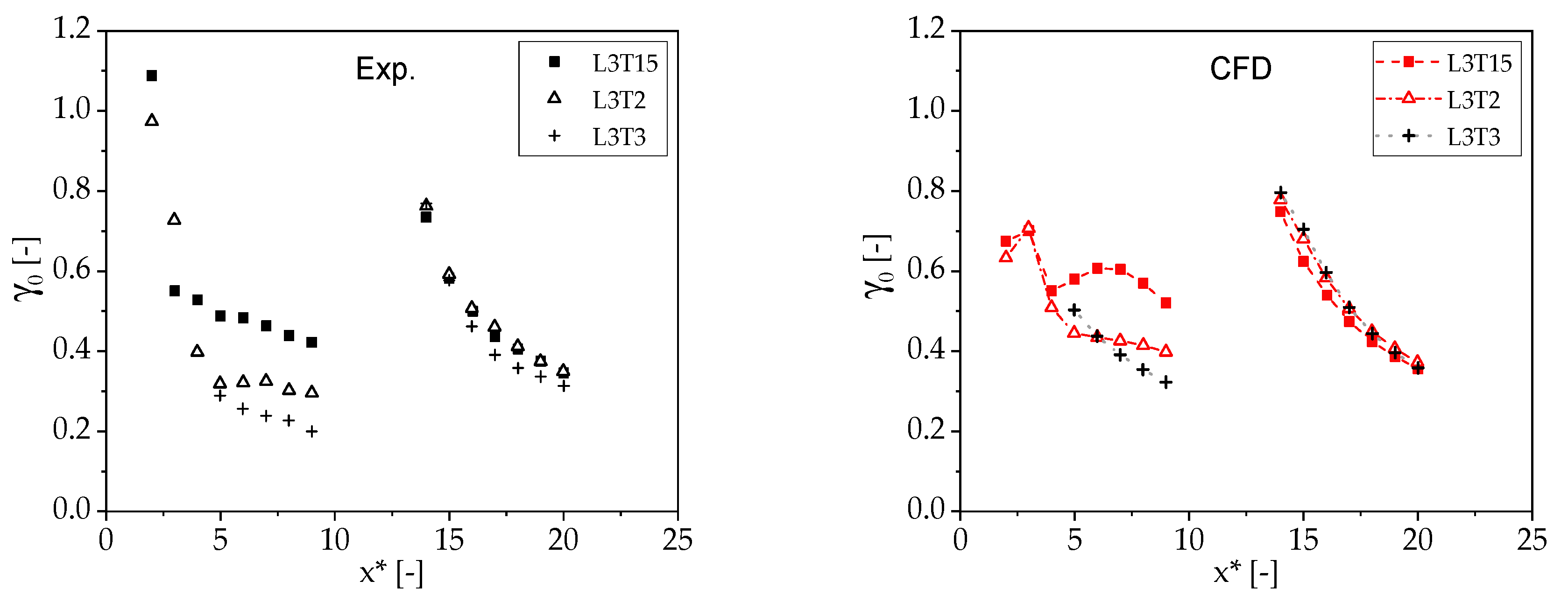
To highlight the ability of the VBM approach to correctly capture the wake velocity gradients measured in the SJTU experiments, all measured and computed γ profiles are grouped in the left and right subplots of Figure 16, respectively. Cross comparison of these two subplots confirms that most wake velocity gradients on the considered centerline are captured adequately by the CFD analyses, particularly so behind the front turbine t1. Both experiments and simulations predict that the fastest recovery of the wake of turbine t1 is achieved with the L3T3 layout. For smaller transverse spacings, the corridor of undisturbed clean flow between the wakes of turbines t2 and t3 becomes too narrow and hinders the recovery of the central wake, which is slowest for the L3T1.5 array, due to the two lateral wakes getting too close and obstructing the way of the central wake, as discussed in further detail below. Both experimental data and numerical results of Figure 16 appear to predict a much lower sensitivity of the t1 rotor wake centerline behind turbine t4 to the lateral spacing of turbines t2 and t3.

The differences between measured data and CFD results noted in Figure 14 and Figure 15 may be partly due to the omission of the supporting frame of the model turbines in the CFD analysis, as the sudden step of this frame on the water path may result in perturbations of the rotor inflow perturbing also rotor wakes. Moreover, Nuernberg and Tao [32], also report that vertical wake displacements in these experiments may also occur due to the vertical shear of the water stream at hub height, which was observed in the experiments. Sheared velocity profiles of the turbine inflow have been shown to affect the wake shape downstream of the turbine by shifting down the wake centerline, due to the velocity shear and reduced wake re-energization, particularly in the case of high seabed roughness [33]. Array simulations carried out including the rotor towers, but not the supporting plates, were also performed to assess the impact of including the towers on the differences between measured data and CFD results. It was found that the inclusion of the towers did not alter significantly the CFD results reported in Figure 14 and Figure 15.

4.2. Turbine/Wake Interactions and Optimal Array Layout

The validation study based on the IFREMER experiments presented above highlighted the VBM capability to consistently predict the power of a turbine operating in the wake of an upstream one. Capitalizing on this outcome, the method is here used to investigate the efficiency of different variants of the four-turbine array module studied in [11], with particular emphasis on the performance of turbine t4 and the design of the array layout that maximizes the array power capture.

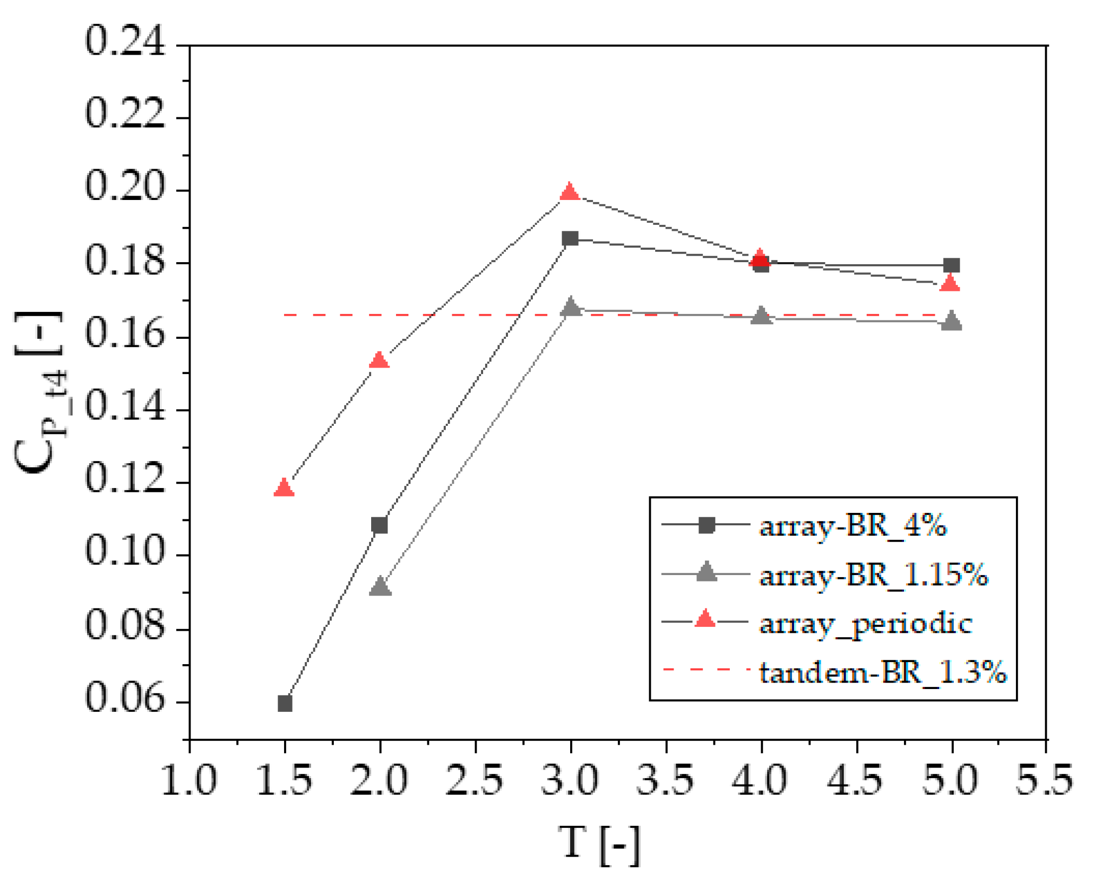
The power coefficient of turbine t4 for some of the considered array layouts, all characterized by the same longitudinal distance of 3D between turbine t1 and turbines t2 and t3, is provided in Figure 17, whose x-axis reports the transverse spacing T of turbines t2 and t3. The curve labeled ‘tandem BR 1.3%’ refers to a simulation in which the width W of the flume tank cross section equals the real value of 3 m, and only turbines t1 and t4 are included; for this reason, this power coefficient estimate of 0.167 does not depend on T. The curve labeled ‘array BR 4.0%’ refers to a simulation in which W is also 3 m but all four turbines are included. In this case, the power coefficient of turbine t4 is lower that than of the two-turbine case for T of 2D or less, it reaches a maximum for T = 3D, and maintains a constant value, higher than that of the tandem case, for T > 3D. The low C_P values for T < 2D are due to the interactions of the wakes of turbines t1, t2 and t3, as discussed below. The fact that for large values of T the value of this variable is larger than that of the tandem case is explained by the influence of the blockage of the tank cross section. To demonstrate this, simulations of the four-turbine array have been performed increasing W to reduce the blockage to 1.15%. The resulting curve is labeled ‘array BR 1.15%’ in Figure 17. It is seen that reducing the blockage, results in the power coefficient of turbine t4 achieving the value of the tandem case as T increases, as expected. This indicates that in an isolated four-turbine array the interactions of the wakes of turbines t1, t2 and t3 cannot be optimized to reduce the losses of turbine t4. However, future arrays will consist of more than four turbines. Therefore, to consider a more realistic future array scenario, the four array simulations have been repeated enforcing a periodicity BC, rather than a solid wall BC, on the lateral boundaries of the tank. In these periodic simulations, the distance between the two periodic boundaries is variable and set to 2T, which is, therefore, also the lateral spacing of the t1 and the t4 turbines. The result is the curve labeled ‘array periodic’ in Figure 17. This curve highlights the existence of a maximum C_P of 0.199 of turbine t4 achieved at T = 3D. As discussed below, this power increase of about 19.16% over the tandem set-up and 6.7% over the BR = 4% wall-bounded four-turbine array is due to a beneficial interaction of the wakes of turbines t1, t2 and t3, and is an effect which may be exploited in the design of full-scale arrays. It is also seen that, as T increases above 3D, C_P decreases again and tends towards the value of the tandem case, as expected.

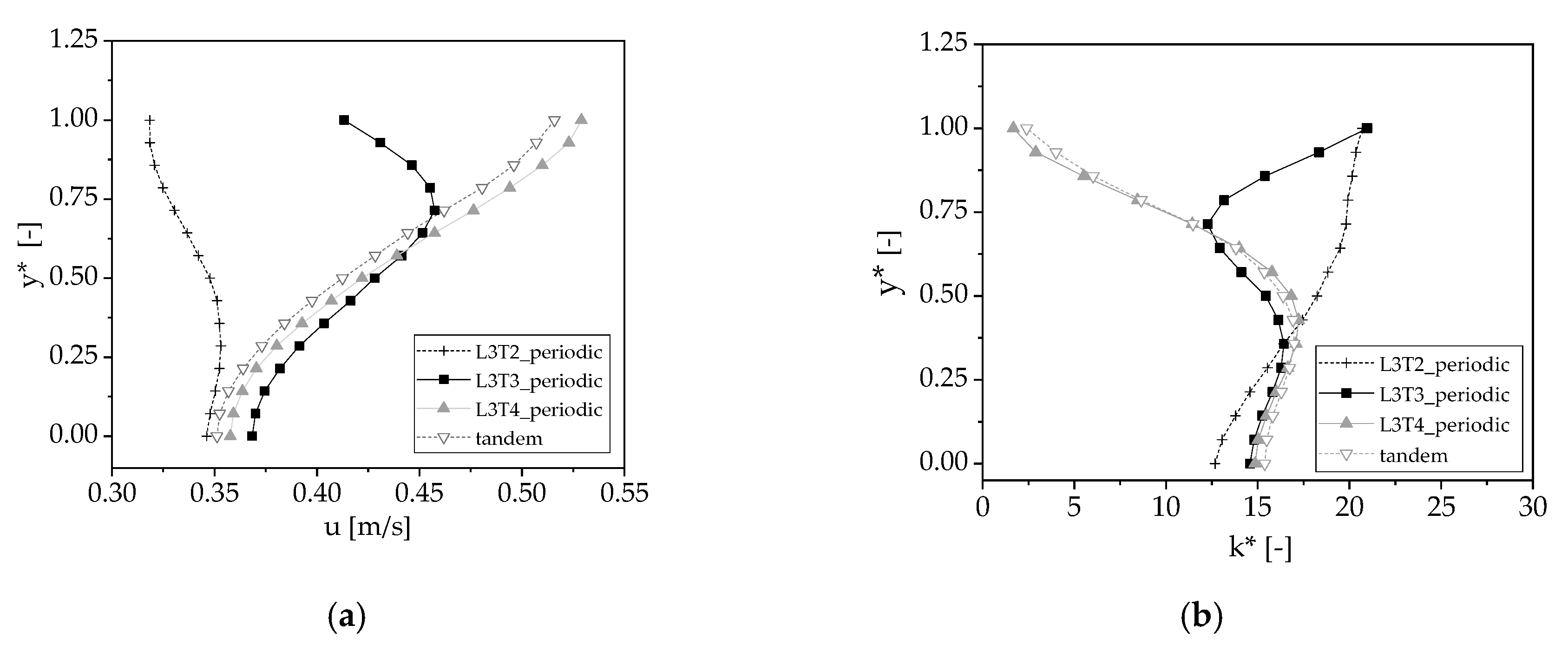
To investigate the dependence of the power of turbine t4 on the transverse spacing of turbines t2 and t3 in a real array, the radial profiles of axial velocity and TKE k* nondimensionalized by the freestream TKE $k_{\infty }$ ahead of turbine t4 for T equal to 2D, 3D and 4D are compared in Figure 18, which also reports the profiles of these variables for the tandem configuration. The variable y* along the horizontal axis is the distance from the rotor axis nondimensionalized by the rotor diameter, so that y* = 0 corresponds to the rotor center and y* = 0.5 corresponds to the blade tip. The first conclusion emerging from the inspection of the velocity profiles of Figure 18a is that the highest axial velocity over the rotor swept area is achieved for T = 3D, which is consistent with the peak power of the periodic array module observed in Figure 17 for this value of T. The velocity profile associated with T = 3D is also higher than that of the tandem configuration. These observations confirm the existence of an optimal lateral spacing T that enables maximizing the acceleration of the wake of turbine t1. It is also observed that the velocity profile of the T = 3D curve has a maximum around y* = 0.75. The velocity reduction for y * > 0.75 corresponds to the outer region of the wakes of turbines t2 and t3. Finally, one also sees that the axial velocity profile for the periodic array module with T = 2D is the lowest one over the entire considered range. This is due to strong interactions of the wakes of turbines t1, t2 and t3, as discussed below in further detail.

Figure 18b provides the radial profiles of k* upstream of turbine t4. One notes that the profiles of the tandem configuration and the four-turbine arrays with T = 3D and T = 4D are very close to each other from the rotor centerline to blade mid-height, that is for 0 < y* < 0.25, indicating that for these values of T, the later turbines have a very small impact on the TKE levels ahead of turbine t4. For 0.25 < y* < 0.50, however, the TKE profile of the T = 3D set-up is lower than the other two, due to the contraction of the wake of turbine t1, which reduces TKE in this region with respect to both the tandem set-up and the T = 4D set-up in which the lateral wakes are not sufficiently close to each other. The shape of the k* profile for T = 2D is due to strong interactions of the wakes of turbines t1, t2 and t3, and discussed below.

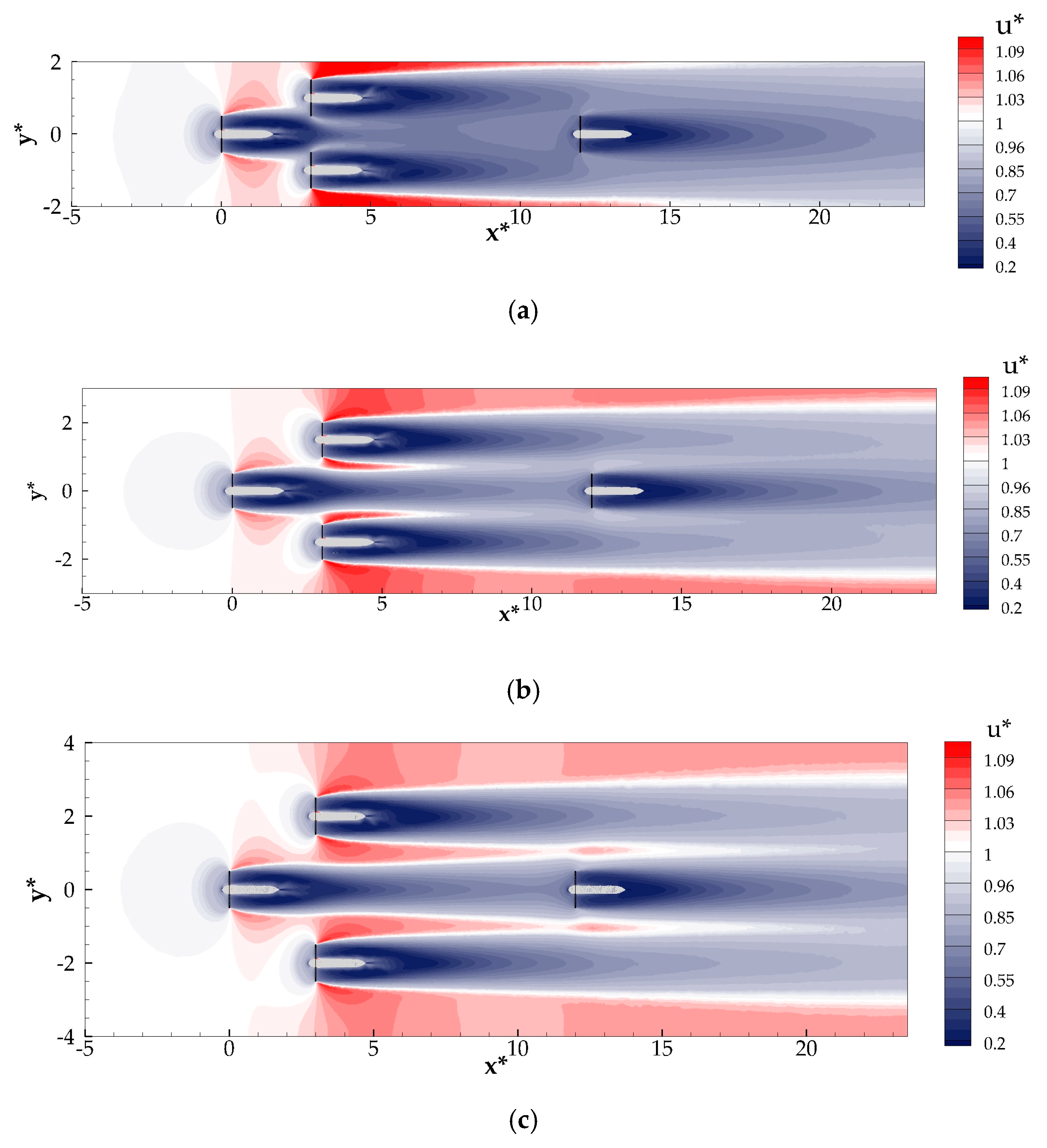
To explain the patterns and relative levels of the radial profiles of axial velocity ahead of turbine t4 reported in Figure 18a it is convenient to examine the contour plots of nondimensionalized axial velocity u* for the considered three four-turbine periodic arrays. The three subplots of Figure 19 provide these contour plots. Figure 19a shows that for the smallest transverse spacing T = 2D, the wake of turbine t1 encounters one side of the rotor of turbines t2 and t3. The main consequence of this is that the wake of turbine t1 experiences strong shearing stresses of the lateral wakes which slow down its recovery, since the wake of turbine t1 is faster than those of turbines t2 and t3 at the axial position where these wakes meet. This effect prevails over the contrasting beneficial acceleration resulting from the increasing contraction of the cross section of the passage between the two lateral wakes as one moves downstream, an occurrence which would tend to accelerate the flow between the two lateral wakes. This explains why the curve labeled ‘L3T2 periodic’ in Figure 18a has the lowest level. For T = 3D (Figure 19b), the wake of turbine t1 is energized when crossing the initial part of the corridor between the wakes of turbines t2 and t3, due to the aforementioned acceleration between the lateral wakes, and this occurrence accelerates the recovery rate of the central wake. In the region between x* = 7 and x* = 8, however, the central wake encounters the less energetic lateral wakes, and this results in slower recovery due to adverse shear stresses on the central wake. Nevertheless, the former effect prevails, and this explains why the velocity profile of this set-up in Figure 18a is higher than that for T = 2D. The velocity reduction of the T = 3D profile of Figure 18a occurring from x* = 0.75 is caused by the merger of the central wake with the less energetic lateral wakes. The contour plots for the array with T = 4D highlight that the central wake does not experience significant shear from the lateral wakes. However, the larger spacing also reduces the acceleration between the lateral wakes, making the evolution of the central wake similar to that obtained without turbines t2 and t3. As a result, the velocity profile of the central wake for this set-up shown in Figure 18a is only marginally higher that that observed with the ‘tandem’ set-up.

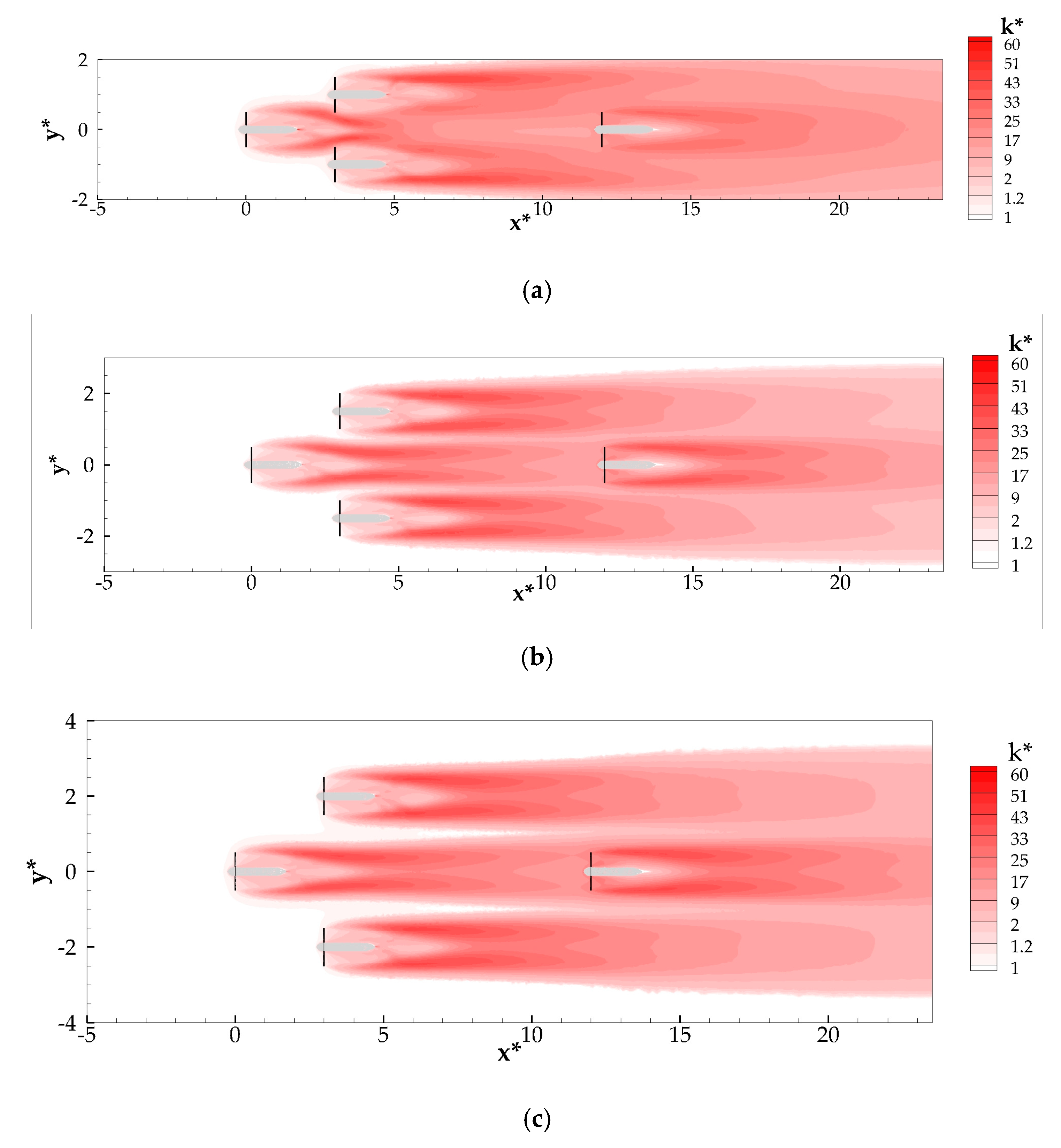
To explain the patterns and relative levels of the k* radial profiles upstream of turbine t4 in Figure 18b, it is convenient to examine the contour plots of this variable for the considered periodic array modules, reported in Figure 20. Figure 20a shows that for the smallest transverse spacing T = 2D, the wake of turbine t1 is intercepted by one side of the rotor of turbines t2 and t3, as already seen in the axial velocity contour plot. At this location, the wake of turbine t1 is throttled and the level of TKE in the central part increases due to diversion of peripheral high-TKE flow towards the centerline of turbines t1 and t4. However, the flow also experiences a strong acceleration around abovesaid centerline, and, as a consequence, the TKE level shortly after the wake encountering turbines t2 and t3 rapidly decreases. This is because of the higher recovery rate promoted by the higher flow speed around the centerline. For this reason, the k* profile of this array in Figure 18b is lower than the other three for 0 < y* < 0.3. Shortly before the rotor of turbine t4, however, the TKE level of the T = 2D array for y* > 0.3 continues to grow and is the highest of all four configurations. This is because the wake of turbine t1 is significantly decelerated by the lateral wakes and partially merges with them. For T = 3D (Figure 20b), the direct interaction between the wake of turbine t1 and the rotor of turbines t2 and t3 is very small. The beneficial acceleration effects on the wake of turbine t1 manifests itself further downstream. Indeed, the cross comparison of the contour plots of Figure 20a,b shows that the TKE level in the outer region of the swept rotor area is lower (lighter red) for the array with T = 3D. This is an effect of the acceleration between the wakes of turbines t2 and t3 which increases the recovery rate of the outer region of the wake of turbine t1. This is the reason why the k* profile of the array with T = 3D in Figure 18b is lower than all other three for 0.3 < y* < 0.75. For y* > 0.75, however, one experiences the high TKE level of the lateral wakes, which is the reason for the rise of this profile in Figure 18b. Similarly to the case of the axial velocity contour plot, the k* contour plot for the array with T = 4D also highlights that the central wake is not affected significantly by the presence of the lateral wakes. Although the k* contour plots of the ‘tandem’ set-up are not reported for brevity, it has been observed that the k* contours past turbines t1 and t4 for the tandem configuration and the four-array set-up are comparable, confirming that for T > 4D the presence of the lateral wakes does not influence significantly the flow upstream of turbine t4.

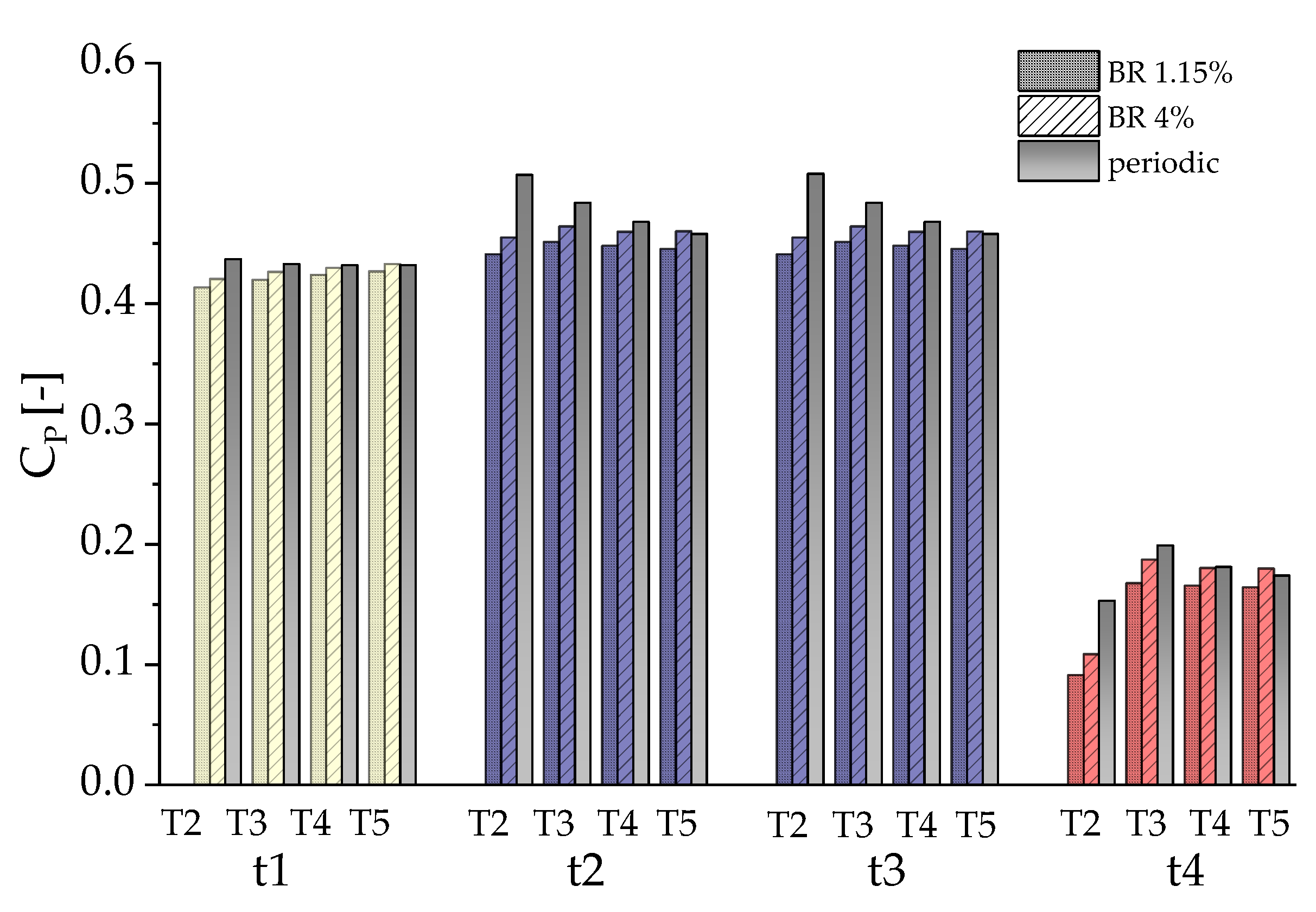
The bar chart of Figure 21 reports the power coefficients of the four turbines of all key array modules considered in this study. Three array module types are considered: one is the wall-bounded array with width of the flume cross section of 3 m, which is labeled ‘BR 4%’, one is the wall-bounded array with artificially increased width yielding a smaller BR, which is labeled ‘BR 1.15%’, and one is the periodic array, labeled ‘periodic’. For each layout type, four values of T are considered, namely 2D, 3D, 4D and 5D. As expected, the smallest sensitivity of the power coefficient to the layout type and lateral spacing is observed for turbine t1. This is because the water speed upstream of this turbine does not vary significantly with these two parameters. For given wall-bounded layout, the power coefficient of turbines t2 and t3 does also not vary significantly with their lateral spacing, due to the low sensitivity of their onset velocity to abovesaid lateral spacing. The power level of these two turbines is slightly higher for the case with higher blockage, which corresponds to the actual dimensions of the flume cross section. In the case of the periodic array, which is more representative of a real multi-turbine installation, the power of turbines t2 and t3 is maximum for the smallest value of T and decreases as this parameter increases. This is because in the periodic set-up the reduction of the lateral spacing T between turbines t2 and t3 also results in the reduction of the lateral spacing 2T between adjacent t1 turbines. Thus, decreasing 2T leads to a stronger flow acceleration between the wakes of the turbines in the front row, and therefore larger power captured by the turbines in the second row. The variation of the water speed upstream of turbines t2 and t3 with T is clearly visible in the four subplots of Figure 19. For all array modules considered, turbine t4 in the third row has the lowest power levels, due to this turbine operating in the low-velocity region corresponding to the wake of turbine t1. However, the power of turbine t4 is also that showing the largest sensitivity to the variations of T. In the case of the wall-bounded array modules, the power increases with T until T = 3D, after which a fairly constant level is maintained. The constant power level achieved at higher values of T is slightly higher for the set-up with BR = 4% corresponding to the actual flume tank width. This observation is important in the design of flume tank experiments aiming at studying turbine/wake interactions and draw guidelines for the design of full-scale arrays. With regard to the design of full-scale arrays with many turbines, however, it is more instructive to consider the case of the periodic module, whose examination shows that the value T = 3D maximizes the power capture of turbine t4, as also shown in Figure 17.

In the design of a full-scale array, one of the objectives is to maximize the power capture of the whole array. A convenient metric to estimate this variable is the mean power coefficient of the periodic array module, noting that the definition of all power coefficients adopted herein implies that these coefficients are all proportional to the turbine power through a common constant. The mean power coefficients of the periodic array module for lateral spacings T2, T3, T4 and T5 are respectively 0.401, 0.400, 0.387 and 0.380. Similar maximum values of the array power are obtained for spacings T2 and T3, and this is because although the power of turbine t4 is maximum for spacing T3, that of turbines t2 and t3 is maximum for spacing t2. Other factors, such as the ease and safety of circulation of marine mammals, may result in spacing T3 being preferred.

5. Conclusions

This study investigated the phenomenon of wake/rotor interactions in tidal stream turbine arrays, and the impact of these interactions on turbine efficiency. The considered case was that of a turbine working in the wake of an upstream turbine wake, with this wake subject to interactions with the wakes generated by two turbines symmetrically positioned to its sides. The numerical analyses were carried out using ANSYS^® FLUENT^® Navier-Stokes computational fluid dynamics analyses, in which the turbines were modelled using a generalized actuator disk model. Validation of the numerical method was based on thorough and comprehensive analyses of two model turbine and model array flume tank experiments, one carried out at IFREMER, the other at Shanghai Jiao Tong University, and comparison of numerical results and measured data in terms of turbine power (IFREMER experiment) and wake velocity and turbulence intensity profiles (IFREMER and SJTU experiments). A very good agreement was found in most cases. Starting from the diamond-shaped layout of the four-turbine array layout of the SJTU experiments, a numerical study was undertaken with the aim of optimizing the spacing of the lateral turbines of this modular array pattern to minimize the power loss of the central downstream turbine and maximize the array mean power by increasing the recovery rate of the wake of the central upstream turbine. It was found that the optimal lateral spacing of three rotor diameters of the two side turbines maximizes the power coefficient of the array and the downstream turbine, enabling the power of this turbine to increase by nearly 20% with respect to the case in which the two side turbines are absent or positioned at larger lateral spacing.