Reinforcement Learning for Optimizing Driving Policies on Cruising Taxis Services


1
Jiangsu Key Laboratory of Urban ITS, Southeast University, Nanjing 211189, China
2
Jiangsu Province Collaborative Innovation Center of Modern Urban Traffic Technologies, Southeast University, Nanjing 211189, China
3
School of Transportation, Southeast University, Nanjing 211189, China
*
Author to whom correspondence should be addressed.
Sustainability 2020, 12(21), 8883; https://0-doi-org.brum.beds.ac.uk/10.3390/su12218883
Submission received: 18 September 2020
/
Revised: 21 October 2020
/
Accepted: 22 October 2020
/
Published: 26 October 2020
(This article belongs to the Section Sustainable Transportation)
Abstract
:As the key element of urban transportation, taxis services significantly provide convenience and comfort for residents’ travel. However, the reality has not shown much efficiency. Previous researchers mainly aimed to optimize policies by order dispatch on ride-hailing services, which cannot be applied in cruising taxis services. This paper developed the reinforcement learning (RL) framework to optimize driving policies on cruising taxis services. Firstly, we formulated the drivers’ behaviours as the Markov decision process (MDP) progress, considering the influences after taking action in the long run. The RL framework using dynamic programming and data expansion was employed to calculate the state-action value function. Following the value function, drivers can determine the best choice and then quantify the expected future reward at a particular state. By utilizing historic orders data in Chengdu, we analysed the function value’s spatial distribution and demonstrated how the model could optimize the driving policies. Finally, the realistic simulation of the on-demand platform was built. Compared with other benchmark methods, the results verified that the new model performs better in increasing total revenue, answer rate and decreasing waiting time, with the relative percentages of 4.8%, 6.2% and −27.27% at most.
1. Introduction
In recent years, taxis service has become blossomed, with worldwide coverage by transportation networks companies such as Uber, Lyft, and DiDi ChuXing [1]. As the convenience and flexibility, compared with the public transportation modes, taxis services profoundly impact residents’ travel behaviours and consequently change the urban transportation system. However, the reality has not shown much efficiency [2]. Specifically, many vacant taxis often wander around the city to find potential orders, while passengers failed to get available cars during particular times in some areas. The imbalance between the supply and demand of taxis has led to mismatches of orders and drivers, causing passengers and drivers to spend more time and money. Furthermore, this phenomenon can result in traffic congestion, consumption of resources, and environmental pollution.
In China, there are two ways of developing taxis services. One way is cruising taxis service organized by taxis companies. The other is ride-hailing platform services such as Uber, Meituan ChuXing, and DiDi ChuXing. Cruising taxis services take up over 60% of total passenger volumes in China in 2019 [3], indicating that cruising taxis are still in the lead. In ride-hailing platform services, drivers usually are restricted to answer orders according to dispatch measures from a unified decision-making platform. They can only handle the orders recommended according to dispatch measures. Consequently, the driving policies are purely determined by the centralized system. When it comes to cruising taxis service, drivers wander around to seek orders. People who require a trip prefer to wait by the streets. When drivers meet passengers, they negotiate the travel and then make a deal. During this progress, drivers receive little advice from the taxis company. Their driving policies usually depend on their experience or temporary situation, which is too subjective and partial to be the optimal decision.
In this paper, we focus on optimizing driving policies for cruising taxis, which increase drivers’ benefits and opportunities for matches of drivers and passengers. Previously, taxi companies widely implemented greedy geographic methods to finish order dispatch, such as searching the nearest driver-passenger pair or using the queueing strategies based on the principle of first-come-first-serve [4,5]. Different objects were aimed to increase taxis services’ efficiency, such as minimization of waiting time, minimization of the distance between the drivers and passengers, maximization of the expected profits, and the probability of finding potential passengers [6,7,8]. Although these works seemed easy and effective, they neglected the spatiotemporal relationship of cars and orders, bringing about a suboptimal consequence when considering in the long run.
To explore optimal strategies, many researchers have investigated the factors influencing the demands and supplies carefully. Four factors included average waiting time, distance, the fare, and the transition probability for recommending a potential high-revenue location were investigated to build a taxi recommender system [9]. The results showed that distance to the next cruising location and waiting time are most essential features. Ji Wang comprehensively studied the spatiotemporal features for taxi route recommendations [10]. They studied the dynamic taxi route recommendation problem as a sequential decision-making problem and designed an effective two-step method to tackle it. A taxi monitoring method is presented to detect anomalous driving behaviours, improving the taxi service [11]. A spatiotemporal data mining framework was proposed to explore mobility dynamics from taxi trajectories [12]. The framework aimed to predict travel demand in different regions of a city efficiently and timely. These works helped us have a good grasp of the factors that improve taxis service.
With information and communication technology tools (ICT) involved [13,14,15], recent works have shown that reinforcement learning (RL) could achieve remarkable results. Gao formulated the optimizing problem as a Markov decision process (MDP) and developed the RL model [16]. The results showed that the method dramatically improves profits and efficiency for cabdrivers. A novel model-free deep reinforcement learning framework was defined to solve the taxi dispatch problem by predicting the number of taxis allocated [17]. Unlike previous researches that mostly focused on using model-based methods, the paper explored the policy-based deep reinforcement learning algorithm as a model-free method. The numerical studies indicated that the model-free model has better performance. At the same time, researches with many deep learning models (i.e., Deep Q Network (DQN), Policy Gradients, Actor-Critic) were proposed to optimize the dispatch between the driver and orders [18,19,20]. They provided reliable optimization policies and expected superb rewards in actual applications throughout the investigated historical taxi trajectory and orders dataset. However, these works mainly focus on the optimization of ride-hailing platform services.
There are two main limitations to those researches:
- (1)
- Order dispatch could profoundly change the spatial and temporal distribution of cars and passengers. The policies without long-term consideration tend to satisfy the current environment, leading to inappropriate matches between drivers and orders. As a result, the optimization might not guarantee global optimization.
- (2)
- Previous research mainly focused on order dispatch to provide optimal driving policies. The information about taxis and orders were indispensable for making policies so that the optimization was concentrated in a unified decision- making framework. For cruising taxis services, the framework was unavailable. Therefore, a single taxi driver cannot take measures without receiving instructions from the central platform.
Our contributions in this paper are as follows:
- Different from the previous works focusing on the orders dispatch on the ride-hailing platforms, our method is studied for the cruising taxis service, which is still useful for a single driver.
- A developed reinforcement framework is proposed. This approach considers long sequences of drivers’ processes in a global environment, so it can guarantee the drivers obtain optimal policies.
- Dynamic programming is employed to reduce complexity, with data expansion algorithm alleviating data sparsity.
- A simulation for the on-demand platform is built to confirm that the model is equally powerful in improving the expected future benefits and increasing the opportunities for matches of drivers and passengers.
The rest of this paper is organized as follows: We provide the system architecture of the proposed model using RL in Section 2. The Experiments and results are then described in Section 3. We analyse the optimal policies in detail and conduct a simulation to verify the superiority in Section 4. At last, Section 5 concludes the paper.
2. Methods
In this section, we firstly describe the optimal problem as the Markov decision process. That is necessary for us to apply reinforcement learning (RL). Then, we develop the RL framework with two novel algorithms. Notations that will be used are listed in Table 1.
2.1. Preliminaries
The Markov Decision Process (MDP) is typically used to model sequential decision-making problems, which is the necessary process of RL. Generally, the MDP can be described by a tuple . Considering a specific state and a specific action at time t, the probability of reaching state s at time t + 1 is determined by transition probability matrix as Equation (1):
Furthermore, the essential part of MDP is that the action selected is purely determined by the current state, which can be described as Equation (2):
There are two types of value function in MDP. One is state value function V(s), another is state-action value function Q(s,a). V(s) represents the expected cumulative future rewards of current state, and Q(s,a) represents the expected cumulative future rewards of taking action a at state s. In standard MDP, agents adapt to the environment by following a policy π, which is mapping from (s,a) to the probability of taking action a at state s. Therefore, under the policy π, V(s) and Q(s,a) are denoted as Vπ(s) and Qπ(s,a) as Equation (3).
Besides, the relation of and are described as Equation (4):
The optimal policy for maximizing the rewards is simply to maximize the Vπ(s). According to Equation (4), the greedy approach is to take the largest one among the (Equation (5)):
Reinforcement learning is a primary approach to learning control strategies by considering what actions intelligent agents should take to maximize a numerical reward signal [21]. RL acquires the best actions in different states by accumulating experience through continuous trial and error training in the environment. Therefore, RL mainly performs much more excellently in the long-term than the short-term [22]. By maximizing the expected cumulative reward in every independent state in constant iterations, RL is adopted to help the agents obtain the optimal strategy in each state. Specifically, after calculating the and , the optimal policies are then determined according to Equation (5).
2.2. Problem Statement and Application
Taxi drivers’ behaviours depend on the current situation instead of previous situations [20]. They mainly care about the current state and the influence of the current action selected. Meantime, drivers are assumed to be resourceful and rational [16], so they are considered to make every decision based on calculation and experience, which means that each decision is the current best strategy. Expressly, drivers accept orders and get passengers from one place to another when they thought this trip deserved. By taking the action of serving the trip, drivers earn money after completing orders. Apart from accepting orders, drivers can also idle when there were neither available orders or worthy orders. The drivers stop or wander around to search for valuable orders. Drivers take actions based on their driving policies. Therefore, we regard the drivers as the agents in MDP, which behave in the environment under the policy that identifies how the agents select actions for maximizing reward. In this paper, we aim to maximize the drivers’ profits in the long run by adjusting the driving policies. Next, the key elements of the driving behaviours as MDP are introduced.
State Space: The state of the driver is defined as a two-dimensional vector representing spatiotemporal status. Each state consists of time and location. Formally, we define . Thus, . In this paper, we discretize the time-space into steps of 10 min and discretize the location space by dividing the area into 500 m × 500 m grid cell, respectively [23].
Action Space: A driver has two available actions in any state, i.e., {idling, serving}. The first type of action is to represent the driver hanging around or waiting in the vacant taxi area. He/she is not matched with any orders temporarily, so he/she can move freely. The last type of action is to assign the driver to serve a specific order. When a driver takes action serving, his/her action cannot change until the order is accomplished. Formally, we define , where 0 means action idling, while 1 means action serving.
Reward: reward means that a driver acquires the profit after taking action and finishing the transition between states. Intuitively, the reward can be represented as an order price. A discount factor was defined to control the degree of how far the MDP looks into the future. The larger factor causes slight future impacts. It is beneficial to use a small discount factor as long horizons introduces a large variance on the value function. Formally, we give the Equation (6) to express this function.
State-action value function: As the optimize object, the state-action value function evaluates driving policies by accumulating every action’s rewards at each iteration. Each action not only determines the immediate reward but also impacts the future reward. It is significant to consider the future reward for global optimization. Mathematically, it is described as Equation (7):
The relation between and are described as Equation (8):
Policy: stores the distribution from a state () to each action () over the action space. The greedy policy was used to learn the best value, .
State value function: It is expected cumulative reward that the driver gains till the end of an episode if he/she starts at state s and follows a policy π. In the learning process, the State function is updated by ; therefore, .
2.3. General Framework
2.3.1. Policy Learning
Generally, policy learning consists of two steps: policy evaluation and policy improvement. Based on the MDP formulated problem above, the optimization can be solved by a model-free approach. Policy evaluation represents the agents continually evaluate the value function from the sample, and the policy improvement gives the better policy for maximizing the rewards.
Policy evaluation: In the policies evaluation step, each agent evaluates the corresponding state value function and state-action value function by taking particular policies. The value function is updated after taking action serving or action idling.
Temporal-Difference (TD) learning is a conventional value update method [24]. This algorithm learns from the incomplete state sequence obtained from sampling. It firstly estimates the possible return of a state through reasonable bootstrapping and then uses progressively updating the average value to obtain the final value. The value of this state is continuously updated through sampling.
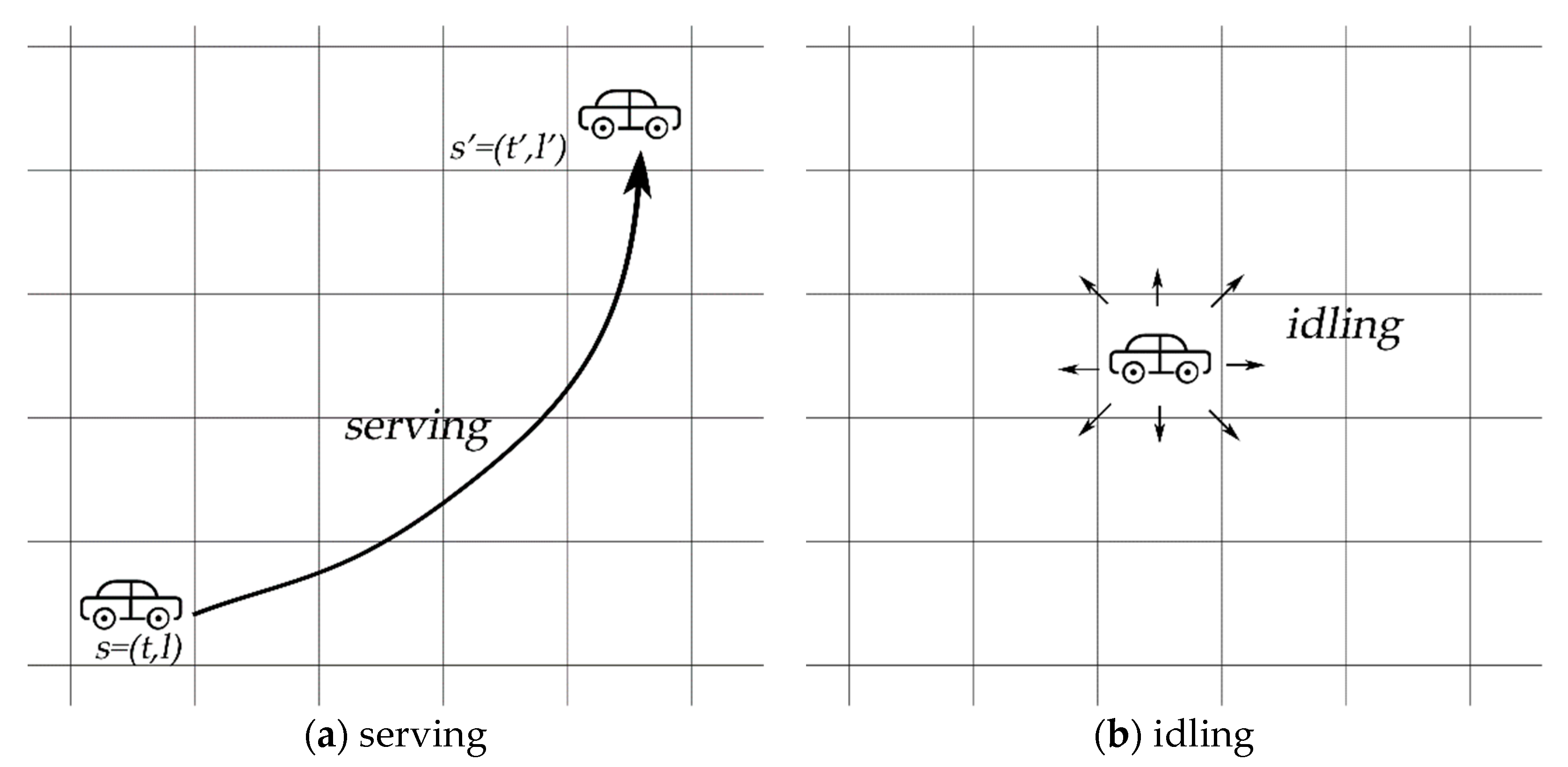
Figure 1 shows the two types of actions. Serving means the drivers receive an order and then proceeded to the destination. Drivers finished the states’ transition from state s to state s’, including the spatial and temporal dimension. As shown in Figure 1a, when taking action serving, the agent goes to the destination and consequently gets a reward. The Temporal-Difference update rule is as follows:
is the current status of the driver, and is the state after completing the order. represents the sum of the estimated time of pickup, waiting, and delivery process, which approximately equals .
When it comes to action idling, an agent can go to the nearby areas and get no immediate reward. They are restricted to wander around nine neighbour grids at most. Therefore, s’ equal s + 1, and l’ must be one of the adjacent grids of the l. The TD update rule is computed as:
Policy improvement: Policies improvement is the optimization stage, corresponding that the agents choose action with the maximum cumulative reward in the current state. The greedy strategy was widely used to determine the best action. It can be described as the following: For every spatiotemporal state , where are learned by policy evaluation.
2.3.2. Dynamic Programming for Policies Learning
Because of massive calculation and iterations, the TD rules seem complicated in this case. The paper develops an implementation based on dynamic programming (DP) to update the value functions. It is suitable to take advantage of the data structure. Drivers take action and then finish the transitions from one state to another. Because of the transitions, the opening state and ending state are connected by the rewards of transitions. For those states with the same locations index, their value function can be calculated by other state whose time index is later. The DP algorithm is executed in an inverted order of time slots. Algorithm 1 describes the process specifically. There are some details needed to be noticed.
- (1)
- At the last time index, the was set zero manually.
- (2)
- The usually does not equal the expected total revenue that drivers earn on average from the current state because of the discount factor.
- (3)
- The set is produced by the vacant drivers’ historic transition probabilities calculated from the trajectory data.
| Algorithm 1: Policy learning using dynamic programming |
| Input: Dataset that stores the historical state transitions pair: |
| Output: , |
| 1: Initialize , , auxiliary matrix as zeros for all state space. |
| 2: Each state consists of a time index and a location index: . |
| 3: K is the maximum time index. |
| 4: for t = K-1 to 0 do |
| 5: Collect subset |
| 6: for each in do |
| 7: |
| 8: if then |
| 9: |
| 10: else |
| 11: |
| 12: end if |
| 13: end for |
| 14: |
| 15: end for |
2.3.3. Transitions Expansion
Some rare states may have an empty historical data set since the orders’ spatiotemporal distribution is uneven. The more specific the divisions of time and space are, the more serious the problems are. Generally, transitions pair could not have the ability to cover the state entirely. The historic orders data may not show all possibilities. In some states, there might be a small amount of orders data starting from there. It is difficult for the RL framework to evaluate the policies sufficiently. In the policy evaluation progress, the corresponding action-state function value could not be calculated correctly. As a result, optimal policies are useless there. In the real world, when a driver goes through a state where few transitions take place, i.e., midnight and remote area, he/she cannot learn from the optimal policies to make good decisions. More training data can significantly reduce the data sparsity. We use a unique method, performing an expanded transitions’ search in both spatial and temporal space to overcome the limitations.
- (1)
- The first search is through spatial expansion. According to Tobler’s First Law of Geography [25], adjacent geographic entities have similar characteristics. If there are no historic orders data that started from , the historical dataset is empty. We search within the same time interval to collect the data from neighbour cells, and those transitions in states were then added to state s ( is adjacent to the ). Notably, a passenger who failed to get a car could go to neighbour grids to seek cars. The same as the actual progress, transitions with the same destination may occur in a nearby area. We can reorganization these transitions to the transition set by replacing with .
- (2)
- The second search is based on temporal expansion. Since the similarity between states with the same location index and approximate time index, this paper considers that transitions pair could also happen as transitions pair where the difference between and is small. An actual case can explain it. A passenger is willing to spend some time waiting for the orders received. Especially in some remote area or low peak period, the time spent might be extended, causing the orders to be placed later.
The two approaches above are established in the hypothesis that passengers are patient enough. Algorithm 2 shows the specific algorithm.
| Algorithm 2: Transitions expand using spatiotemporal search |
| Input: Dataset that stores the historical state transitions pair: |
| Output: Expandable transitions set |
| 1: Initialize |
| 2: State space , parameter |
| 3: for each in do |
| 4: Collect subset |
| 5: if then |
| 6: Spatial Search: |
| 7: Find nearby location index set , is the manhattan distance between and . |
| 8: for in do |
| 9: if then |
| 10: Random choose from , add to |
| 11: go to line 3 |
| 12: End if |
| 13: End for 1 |
| 14: Temporal Search: |
| 15: for in max(0,) to min( K −1, ) do |
| 16: if then |
| 17: Random choose from , add to |
| 18: go to line 3 |
| 19: End if |
| 20: End for |
| 21: End if |
| 22: End for |
| 23: |
3. Case Study
We utilized the historic orders data in Chengdu to represent how the RL frameworks optimize the driving policies.
3.1. Data Description and Preprocessing
The taxi orders data collected from Didi ChuXing taxi company has 6,105,003 pieces of record from the 1st to 30 Nov 2016 in Chengdu city, China. The single-piece data include order ID, pickup time, drop-off time, pickup location, drop-off location, and order price. The order price is not the actual price but calculated as evaluated value by DiDi Chuxing’s algorithm.
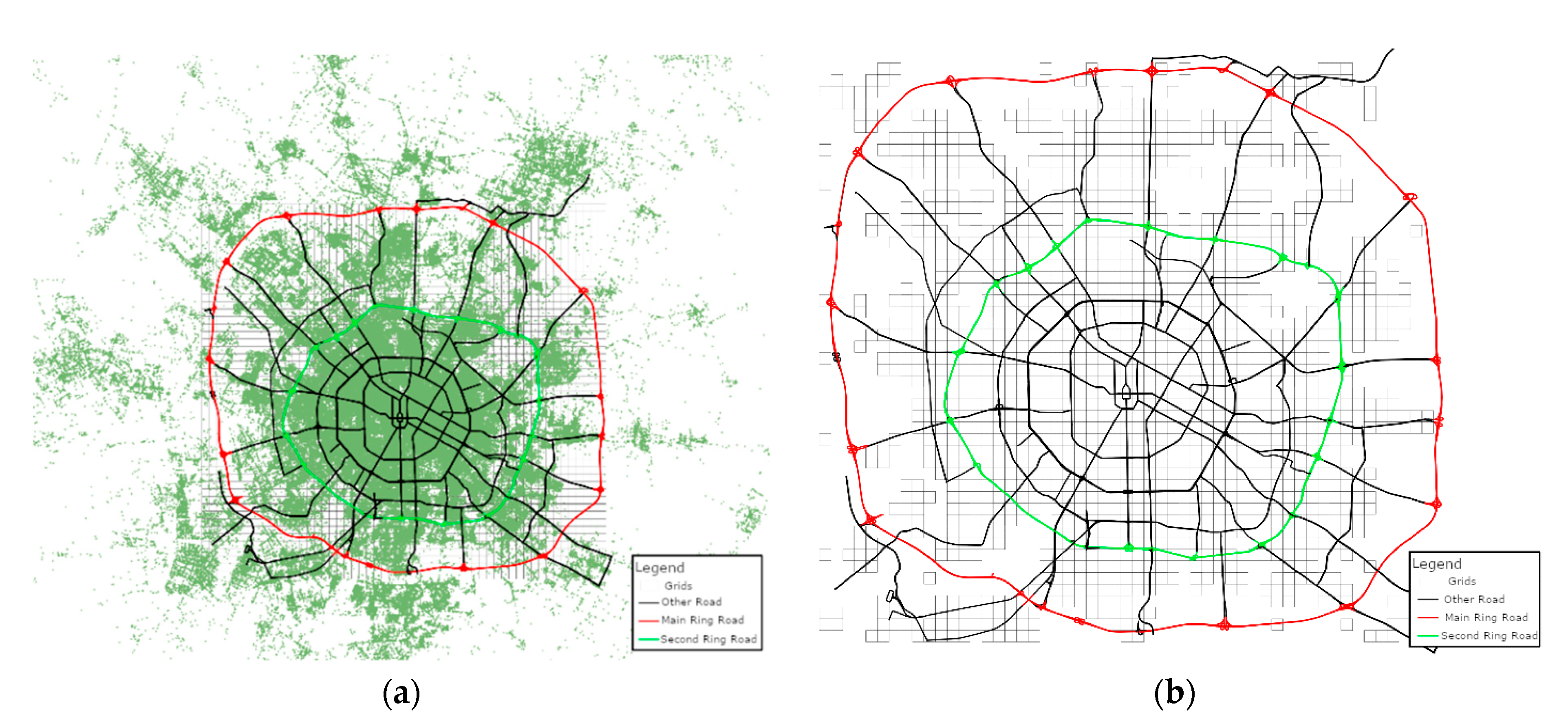
The main road networks in Chengdu was collected as the background data (Figure 2a). The research region of Chengdu was then divided into 500 m × 500 m grids for spatial discretization. There were 2700 grids, covering approximately 678 km2. Approximate 5 million pieces of records fall in the research area. Lack of historic orders originating from there, some grids must be removed. Finally, 1482 grids were left for further experiments (Figure 2b).
The orders data could be easily broken down into the transition dataset. A set of transition pairs was then collected from the historic orders data. Transitions of the first 23 days in the dataset are utilized for training, and the others are left as validation dataset. We focus on the general solution for all agents, so the driver’s identity was not distinguished, supporting that transactions for all drivers form a single dataset. It is consistent with that all agents are trained in one progress of policy learning. Notably, the training data for the proposed model are required to reflect the passengers’ demands. Agents learn from historical experiences to evaluate rewards, caring about the value of transitions instead of the mode. In other words, the model is flexible that the optimization for cruising taxis also takes effects in the ride-hailing platform services equally.
3.2. Application Results
The transition data were utilized for policy training. The value function and in each state were computed iteratively by the RL model. The minority of state, or may be zero due to the lack of training data. In these states, the missing values demonstrate that the policies can be affected by the current dataset. If at least one state-action value in one state is obtained, the policy improvement still works because the maximum one is regarded as the optimal option. This case may be explainable as the drivers always prefer the optimal option. If are both zero in one state, the is also zero owing to the greedy strategy, which means that no policy can be deduced. Using the transition expansion algorithm helps reduce missing situations. Without transitions expansion, approximately 12% of the states had missing values. After using the expansion, the rate of the incomplete states declined to 5%. More training data can significantly reduce the incompleteness.
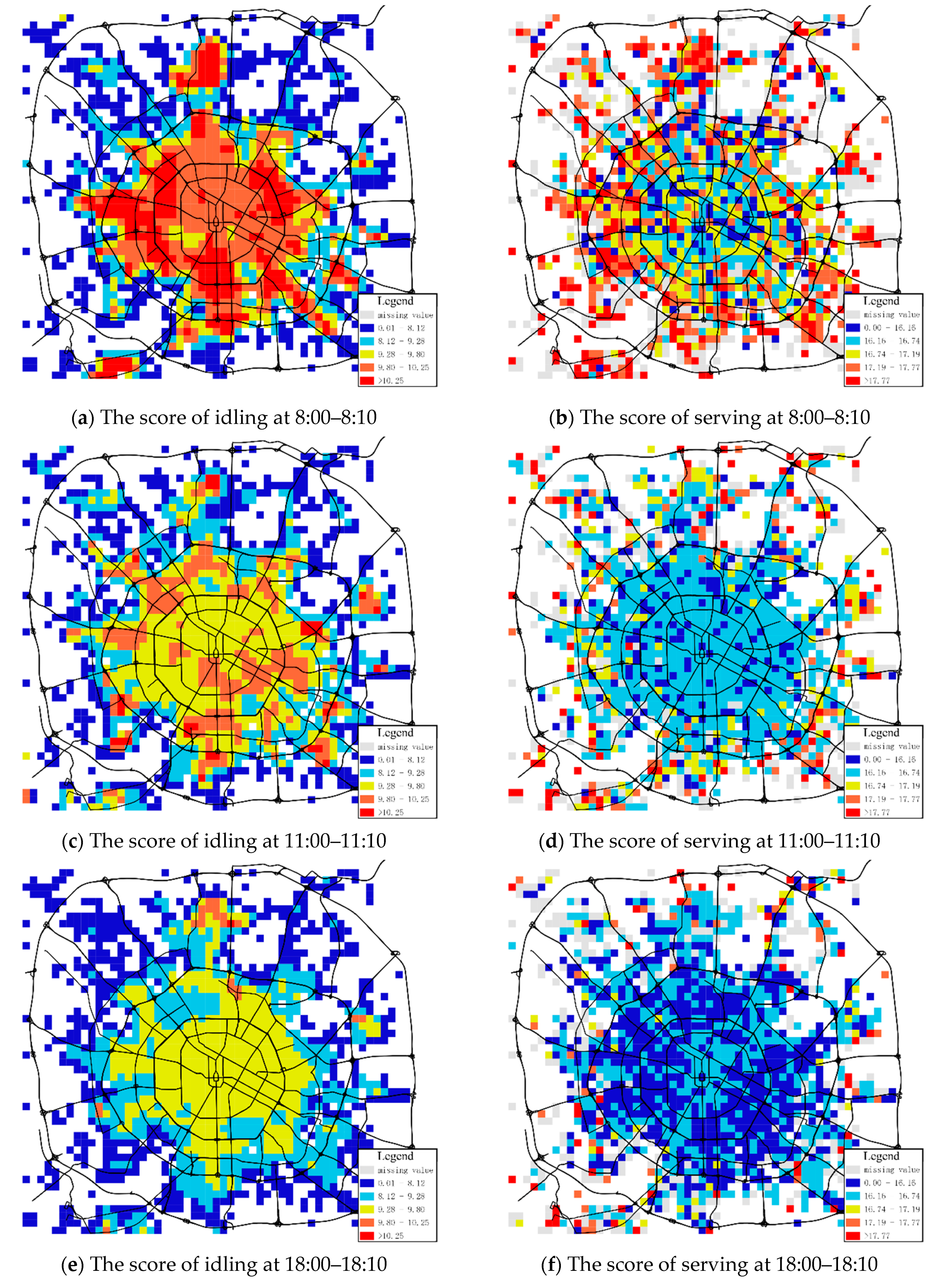
It is difficult to reveal the optimal policies by showing directly as the state space is two-dimensional. To better reflect the results, we showed the distribution of spatial dimensions by fixing the temporal dimension. Three-time indexes representing 8:00–8:10 (morning rush hour), 11:00–11:10 (daytime hours) and 18:00–18:10 (night rush hour) were selected by design.
As shown in Figure 3, the evaluating actions serving and idling, are assigned to each grid cell at a particular period respectively. Notably, figures used different legends since has excessive discrepancies in different figures. Quantile classification was applied for better visualization. At the same period (i.e., Figure 3a,b), action idling receives a high score in an urban area, but the action serving usually receives higher scores in the suburbs, especially around the second ring road. More passengers’ resources in urban areas suggest it is more worthwhile for drivers to idle around, seeking potential orders. Thus, the idling action chosen can eventually bring more profits over the long run.
On the other hand, the highest scored areas of serving are mostly distributed around the second ring road. In these areas, passengers are likely to go to more remote areas, leading to long-distance trips and higher rewards. Besides, the cells with high values of idling action distribute in areas where transportation hubs are located. The cells with high action serving values have wider distribution, which explains the hot spots on the ride-hailing services.
As Figure 3a,b shown, during the 8:00–8:10, the idling scores formed a hot spot in the central city, while the high score of serving was mainly distributed in the main outer ring. In other periods, the spatial pattern appears similarly, with small differences in the details. This phenomenon can be explained by the fact that drivers prefer to idle in the central area because of the higher answer rate. Respectively, the higher prices of orders in remote areas attract drivers to take action serving.
It is worth noting that the value of will be smaller overall as time goes by. The reflects the expected cumulative return in this state to some extent. There is a long-time-interval to the end, so the driver has more opportunities to complete the orders.
Except for the results above, we also discovered some interesting phenomena from the distributions. For instance, there is a small region with high in the north of Chengdu. This phenomenon shows that there is a high demand for taxis during the morning peak period. By analysing these areas with high scores, we can explore potential hot spots for urban traffic. Another strange example is in Figure 3a. According to the analysis above, central areas are more valuable than other areas. However, some grids with low appear in the very central city. At 8:00, many taxis have moved to destinations by the orders answered, which might cause that vehicles are far more than orders in some grids. In that case, drivers have to grab orders with other active drivers. The value of action serving becomes lower than in nearby areas, consequently.
3.3. Optimal Policies Analysis
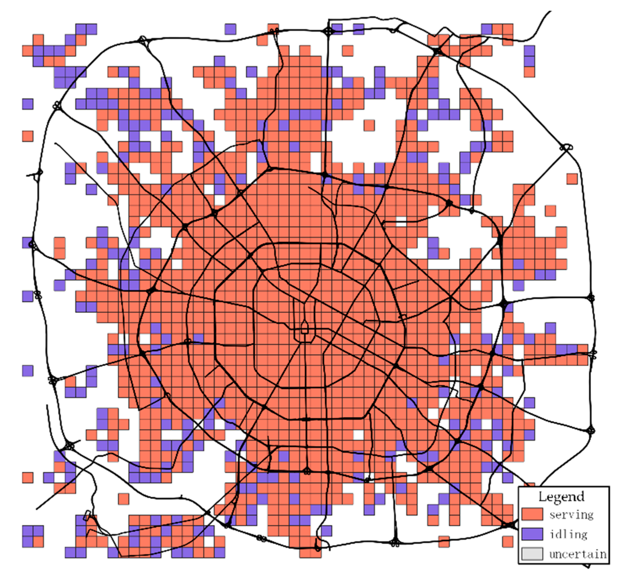
As Figure 4 is shown, the action with the maximum value is preferred as the optimal action. In this period, grids whose optimal policy is serving occupy most of the central city. According to these optimal policies, drivers can determine their driving actions in any state. For example, when vacant drivers start in a specific state, this state’s highest valued action will be recommended. (1) If the value of serving is higher than value of idling, drivers prefer to receive orders if possible and pick up the passengers to the destination. However, drivers have to take action idling when there are no available orders. (2) If the action idling should be chosen, drivers head to one of the neighbour grids with the highest state function value in the next time index. (3) When drivers are carrying on the passengers, they must drive directly to the destination. Drivers are not allowed to make other choices, no matter which action is highest in the cells traversed. After finishing the orders at the ending state, drivers return to the vacant state and then follow the previous description’s optimal policies. Optimizing policies only take effects on the vacant drivers. The optimal action in the current state was chosen, influencing the following states and choices and forming a behavioural decision chain in the long run.
As Figure 5 shown, the difference between the two types of action value is further explored. The smaller the difference, the more serving is superior to idling. The most excellent grids for serving are distributed mainly in the centre of the city, and the score declines outward. The grid with the highest score has some sporadic distribution on the edge of the city. So, it is a wise choice to take action serving in an urban area while taking action idling is better in marginal areas. For example, when a driver has a lower serving utility, he/she may even be unwilling to answer the orders since the value function tells that idling could bring a simple higher monetary revenue. Based on the differences, drivers can quantity their expected profits of taking one specific action than another.
4. Simulation
An example by simulating the real world was designed to illustrate the capacity in handling spatiotemporal optimizing problem.
4.1. Simulation Setup
We imitated the interaction between drivers and orders for an entire day in a virtual environment constructed by 2700 grids with 5 min each step. For data generation, we aimed to build the environment positively reflect the realistic traffic patterns. We used the demands from the test dataset. Orders’ information (starting location, starting time, ending locations, ending time, price) was utilized to generate the orders’ requests. Drivers’ actions were determined by the simulator, computing the system results under different driving policies.
The simulation’s fundamental details are organized here:
- (1)
- At each time step, the framework adjusts vacant drivers’ actions according to the policies, while drivers carrying passengers are not the adjustment objects until they finish orders. In each step, vacant drivers have to take two actions: answer order or idle around (staying or moving to one of the neighbour grids). A driver carrying passengers cannot take other actions until he/she arrives at the destination. Drivers are restricted from moving vertically or horizontally.
- (2)
- The road conditions are assumed to be similar to the history, so we use the historical travel time to represent the simulated travel time.
- (3)
- An order is cancelled if not being answered by any driver for 10 min. An order is matched to the driver when they are in the same grid, respectively.
- (4)
- Taxis are temporarily unavailable during the off-shift periods, so we simulate this situation by shift Change algorithm, which is proposed by Mustafa Lokhandwala (the same setting can be found in that paper) [26].
- (5)
- All the taxis enter the system at the beginning. The set makes little impact on the simulated results because the demand between midnight and the morning rush hour is very low. During this period, the system has enough time to self-balance the available taxis. The number of taxis was 7000, approximately the number of current taxis in the historical dataset.
- (6)
- The time required for refuelling was considered to be negligible.
We compared the proposed method with four basic methods—a random method, a historic-based method, a primary RL method [16], a proposed method without expansion. The random method applied random policy to select actions and movements. The historic-based method collected the transfer probabilities from the historical data and then made the vacant drivers moving to near grids by the probabilities. According to realistic policies followed by temporary accidents or drivers’ experiences, the random method and historical method were set to reflect the actual situation. The primary RL model was applied for optimizing policies in a simple architecture. The primary model considered the spatial dimension without a temporal dimension. The proposed method without expansion was set to show the excellence of data expansion. For quantitative comparison, the paper concentrated on the answer rate, the total revenue of all drivers and average waiting time. Furthermore, seven experimental groups using different day data from the test dataset were examined for avoiding contingency (there are approximate 170,000 orders on the average every day). The final average values were regarded as evaluation indicators.
4.2. Simulated Result and Discussion
Table 2 shows the comparison results of the five methods. It is not astonishing that the random method and historic-based method performs similarly, with the lowest scores of the three evaluated indicators among methods. The policies that depend on historical experiences and temporal situation suggest the low effectiveness of the purposeless account. The primary RL method even performs worse, which indicated that the RL framework might not be applied in a simple architecture. The primary RL method considers the problem without the time dimension. The policies obtained are optimal most time, but they cannot guarantee the effectiveness for a whole day. Although RL takes advantage of handling the MDP progress, we still need to understand it thoroughly. Otherwise, the RL framework may produce error optimization. The proposed method without expansion has slight improvements thanks to active regulation. However, compared with the proposed method, the method without expansion is not effective in the long run. Lack of essential data expansion, the policies obtained cannot explore the state sufficiently. Therefore, drivers receive no optimal strategies in some states, resulting in that overall optimization does not go far enough. The developed RL method achieves the best answer rate, total revenue and waiting time. The results are consistent with our optimal goal that a farsighted consideration improves the overall performance.
We also use the relative percentages in Table 3. The relative value is computed as Equation (11):
where is the relative percentage, is the value of indicator obtained from the proposed RL method, is the value obtained from the compared method.
The proposed method achieves an increase of 4.8% in answer rate, an increase of 6.2% in total revenue and a decrease of 27.27% in waiting times at most (primary RL method is not compared due to its error optimization). Although the improvements seem slight, the proposed method presents a novel way of optimizing driving policies for cruising drivers when most researchers consider order assignment and dispatch. We could further achieve more significant improvements by investigating more spatial and temporal features.
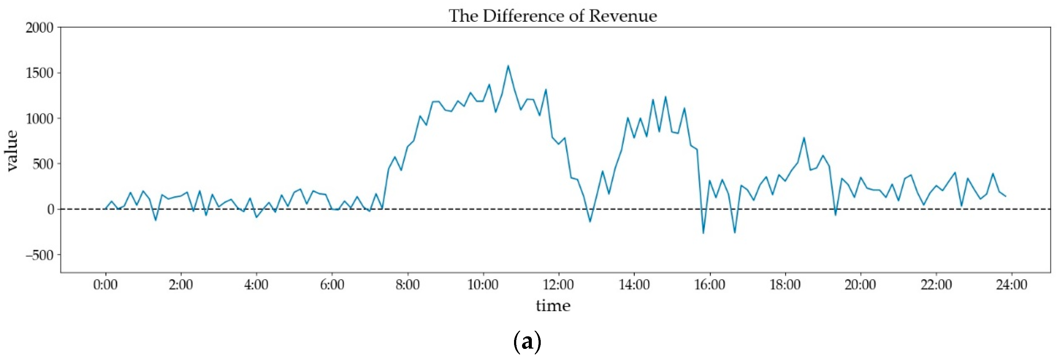
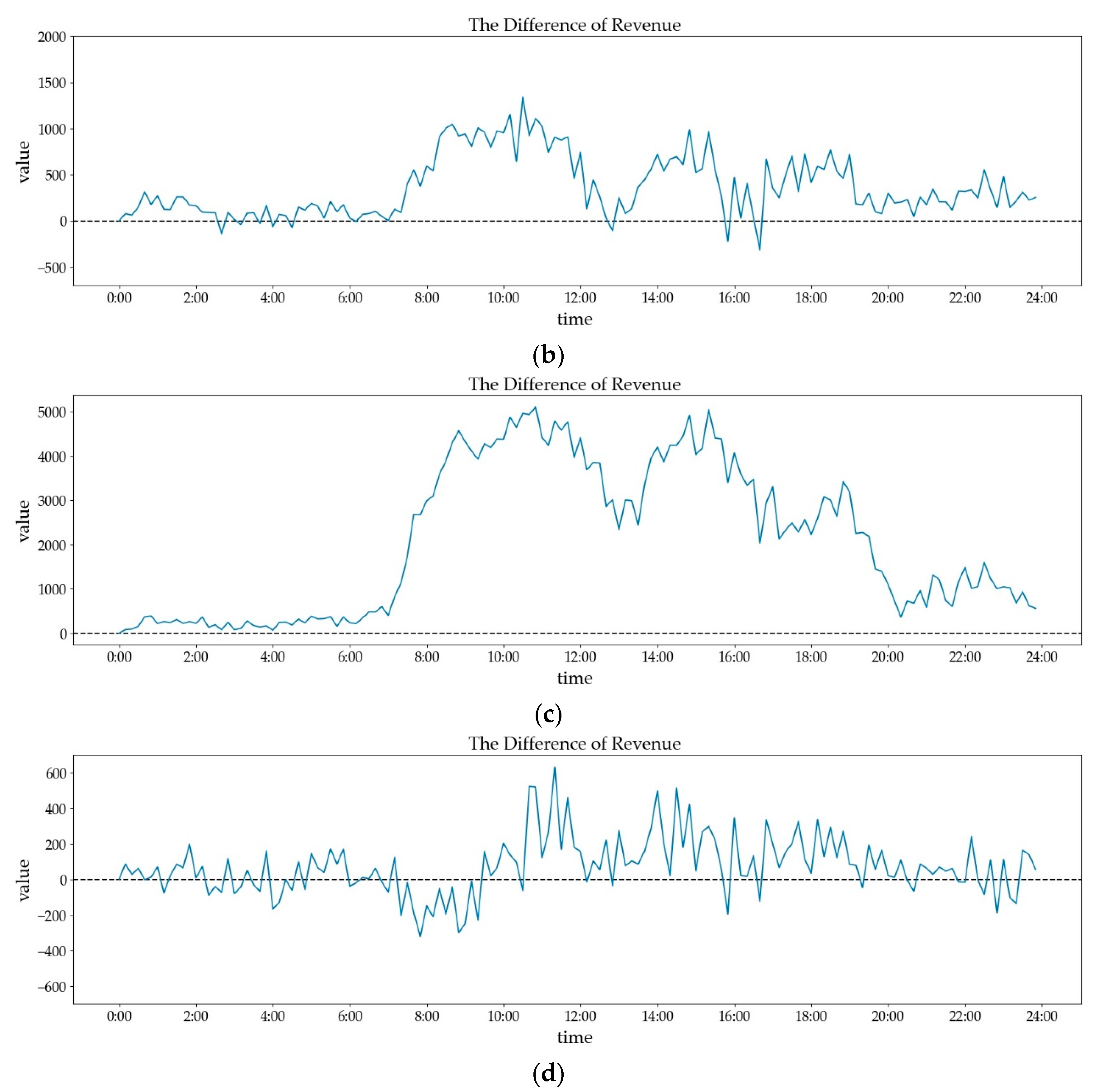
Figure 6 presents the differences in revenue among the RL method and other methods in each time step. Axis X is the time, and axis Y is the difference of revenue during a specific period. The larger the difference is, the higher the proposed method’s revenue gets in a single time step. It can be seen that the RL method acquire higher revenue than the random method and historic-based method in most time (Figure 6a,b), especially in 10:00–11:30, 14:00–15:00 and 18:00–19:00. There are amounts of order requests so that optimal policies can produce significant impacts on the revenue. In 0:00–6:00 (night time), order requests are too few to cause an enormous difference. There are few low peaks at 13:00 (afternoon peak), 15:50 (before evening peak), and 16:20 (evening peak) when random policies and historic-based method has better revenue than the RL method. It can be explained that the random method and historic-based method sometimes focus on the best choice in the current view, with higher profits consequently. It is no doubt that the proposed method is better than the primary RL method overall (Figure 6c). When comparing the proposed method with proposed method without expansion (Figure 6d), we can find that the former has sight improvements than the latter. Although the curve fluctuates around y = 0, the difference is above 0 in most time. The proposed method without expansion is unstable in offering policies, so it eventually is lower than the proposed method.
4.3. Sensitivity Analysis
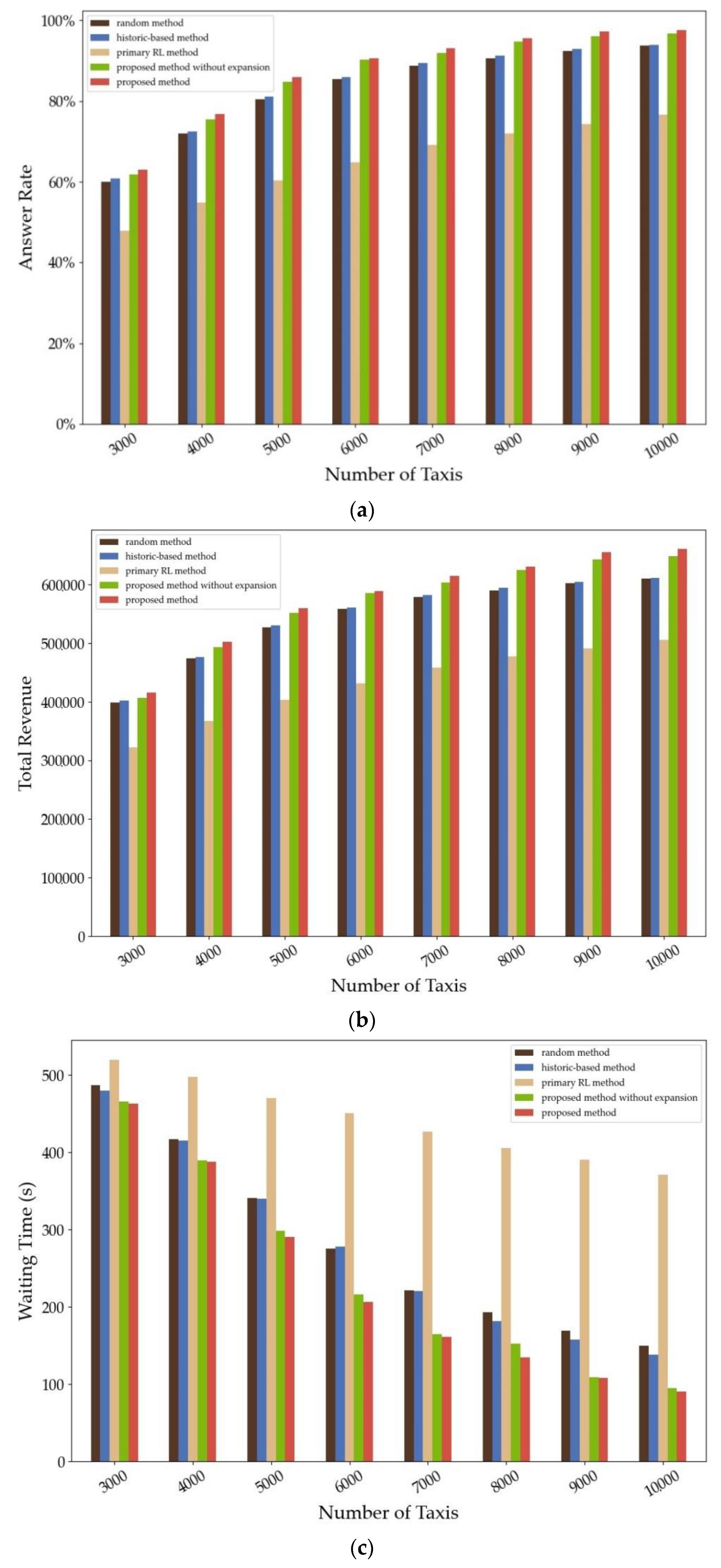
We ran several scenarios for analysing the sensitivity of the number of taxis (Figure 7). We set different taxis numbers from 3000 to 10,000 with 1000’s step. It is not surprising that as the number of taxis increase, answer rate and total revenue all increase, while waiting time decreases. Similar ranks appear in each scenario: the proposed RL method has the best performance, with the method without expansion ranks second. Random method and historic-based method perform similarly, while the primary method is underperformance all along. When the taxis’ number is less than 7000 (the current number of taxis in real world), the three indicators have poor values. Especially when the number of taxis is 3000 (much less than 7000), the indicators are much lower than those in scenarios 7000. With the extreme unbalance of orders and taxis, the orders are too massive to match available taxis. Therefore, the policies have little space to achieve the expected optimization. Besides, as the number of taxis increases, the improvements gradually become smaller. With the number of taxis increase, the spatiotemporal unbalance between orders and taxis are smaller. The majority of orders can be answered successfully, so the influences of optimal policies are narrow.
The results show that the proposed method performs best among the compared methods in each scenario. The paper suggests how effective the proposed method works in environments with a different number of taxis through the sensitivity analysis.
5. Conclusions
This paper proposed a novel method falling within reinforcement learning to optimize the driving policies on cruising taxis services to pursue the maximum profits of drivers and increase the match rate of drivers and passengers. By formulating the drivers’ behaviours to the MDP process, TD update rules using dynamic programming and data expansion were applied to calculate the state-action function value. The proposed method is model-free and globally optimal, thus avoiding that optimal policies fall into suboptimal. The paper uses the historic orders data to recommend the optimal choice of idling and serving to drivers at a particular location and time. A simulation environment was also built to perform detailed modelling of the physical world for the on-demand platform. The results indicated that the proposed method has reasonable improvements over other benchmark methods, which provided useful strategies for drivers and system. We also conducted a sensitivity analysis to figure out how effective the proposed method works in scenarios with different taxis’ numbers.
From the results of the case study and simulation, the main conclusions are made as follows:
- Drivers usually receive more profits when they take action idling in an urban area than in the suburbs. However, in the ring roads, action serving is more valuable than in urban areas.
- The optimal results help explore the transportation pattern in urban transportation.
- The proposed RL model is proved to be realistic to improve the whole platforms’ total revenue and increase the orders’ answer rate.
- We can quantify the advantages over other approaches through the revenue’s difference and sensitivity analysis.
However, this method can be further improved by investigating a more detailed dataset. More temporal and spatial features may be utilized to enhance performance. Besides, we can develop the RL on riding-hailing taxis services in the future. Big data and high computing abilities can also improve the efficiency and accuracy of reinforcement learning. The competitions from other modes are also interesting research points.
Author Contributions
Conceptualization, K.J., W.W. and X.H.; methodology, K.J.; software, K.J.; validation, W.Z.; data curation, W.Z. and K.J.; writing—original draft preparation, K.J.; writing—review and editing, J.K., W.W. and X.H. All authors have read and agreed to the published version of the manuscript.
Funding
This research was funded by the National Natural Science Foundation of China (project no.: 51878166 and 71801042), and the Natural Science Foundation of Jiangsu Province (BK20180381).
Acknowledgments
The authors are grateful to Didi Chuxing (https://gaia.didichuxing.com), which provided the raw data.
Conflicts of Interest
The authors declare no conflict of interest.
References
- Shared, Collaborative and on Demand: The New Digital Economy. Available online: https://www.pewinternet.org/2016/05/19/the-new-digital-economy (accessed on 28 September 2019).
- Baghestani, A.; Tayarani, M.; Allahviranloo, M.; Gao, H.O. Evaluating the Traffic and Emissions Impacts of Congestion Pricing in New York City. Sustainability 2020, 12, 3655. [Google Scholar] [CrossRef]
- Annual Report on China’s Sharing Economy Development. Available online: http://www.sic.gov.cn/News/557/9904.htm (accessed on 28 September 2019).
- Zhang, W.; Honnappa, H.; Ukkusuri, S.V. Modeling urban taxi services with e-hailings: A queueing network approach. Transp. Res. Part C Emerg. Technol. 2020, 113, 332–349. [Google Scholar] [CrossRef] [Green Version]
- Zhang, R.; Pavone, M. Control of robotic mobility-on-demand systems: A queueing-theoretical perspective. Int. J. Robot. Res. 2016, 35, 186–203. [Google Scholar] [CrossRef]
- Yuan, N.J.; Zheng, Y.; Zhang, L.; Xie, X. T-Finder: A Recommender System for Finding Passengers and Vacant Taxis. IEEE Trans. Knowl. Data Eng. 2013, 25, 2390–2403. [Google Scholar]
- Powell, J.W.; Huang, Y.; Bastani, F. Towards reducing taxicab cruising time using spatio-temporal profitability maps. In Proceedings of the International Conference on Advances in Spatial & Temporal Databases, Minneapolis, MN, USA, 24–26 August 2011. [Google Scholar]
- Ge, Y.; Xiong, H.; Tuzhilin, A.; Xiao, K.; Gruteser, M.; Pazzani, M. An Energy-efficient Mobile Recommender System. Soft Comput. 2010, 18, 35–49. [Google Scholar]
- Hwang, R.-H.; Hsueh, Y.-L.; Chen, Y.-T. An effective taxi recommender system based on a spatio-temporal factor analysis model. Inf. Sci. 2015, 314, 28–40. [Google Scholar] [CrossRef]
- Luo, Z.; Lv, H.; Fang, F.; Zhao, Y.; Liu, Y.; Xiang, X.; Yuan, X. Dynamic Taxi Service Planning by Minimizing Cruising Distance Without Passengers. IEEE Access 2018, 6, 70005–70016. [Google Scholar] [CrossRef]
- Ghosh, S.; Ghosh, S.K.; Buyya, R. MARIO: A spatio-temporal data mining framework on Google Cloud to explore mobility dynamics from taxi trajectories. J. Netw. Comput. Appl. 2020, 164, 102692. [Google Scholar] [CrossRef]
- Ji, S.; Wang, Z.; Li, T.; Zheng, Y. Spatio-temporal feature fusion for dynamic taxi route recommendation via deep reinforcement learning. Knowl. Based Syst. 2020, 205, 106302. [Google Scholar] [CrossRef]
- Musolino, G.; Rindone, C.; Vitetta, A. Passengers and freight mobility with electric vehicles: A methodology to plan green transport and logistic services near port areas. Transp. Res. Procedia 2019, 37, 393–400. [Google Scholar] [CrossRef]
- Croce, A.I.; Musolino, G.; Rindone, C.; Vitetta, A. Sustainable mobility and energy resources: A quantitative assessment of transport services with electrical vehicles. Renew. Sustain. Energy Rev. 2019, 113, 109236. [Google Scholar] [CrossRef]
- Croce, A.I.; Musolino, G.; Rindone, C.; Vitetta, A. Transport System Models and Big Data: Zoning and Graph Building with Traditional Surveys, FCD and GIS. ISPRS Int. J. Geo-Inf. 2019, 8, 187. [Google Scholar] [CrossRef] [Green Version]
- Gao, Y.; Jiang, D.; Xu, Y. Optimize taxi driving strategies based on reinforcement learning. Int. J. Geogr. Inf. Sci. 2018, 32, 1677–1696. [Google Scholar] [CrossRef]
- Shou, Z.; Di, X.; Ye, J.; Zhu, H.; Zhang, H.; Hampshire, R. Optimal passenger-seeking policies on E-hailing platforms using Markov decision process and imitation learning. Transp. Res. Part C Emerg. Technol. 2020, 111, 91–113. [Google Scholar] [CrossRef] [Green Version]
- Mao, C.; Liu, Y.; Shen, Z.J.M. Dispatch of autonomous vehicles for taxi services: A deep reinforcement learning approach. Transp. Res. Part C Emerg. Technol. 2020, 115, 102626. [Google Scholar] [CrossRef]
- Wang, Z.; Qin, Z.; Tang, X.; Ye, J.; Zhu, H. Deep Reinforcement Learning with Knowledge Transfer for Online Rides Order Dispatching. In Proceedings of the 2018 IEEE International Conference on Data Mining (ICDM), Singapore, 17–20 November 2018; pp. 617–626. [Google Scholar]
- Xu, Z.; Li, Z.; Guan, Q.; Zhang, D.; Ke, W.; Li, Q.; Nan, J.; Liu, C.; Bian, W.; Ye, J. Large-scale order dispatch in on-demand ridesharing platforms: A learning and planning approach. In Proceedings of the 24rd ACM SIGKDD International Conference on Knowledge Discovery and Data Mining, London, UK, 19–23 August 2018. [Google Scholar]
- Jameel, F.; Javaid, U.; Khan, W.U.; Aman, M.N.; Pervaiz, H.; Jäntti, R. Reinforcement Learning in Blockchain-Enabled IIoT Networks: A Survey of Recent Advances and Open Challenges. Sustainability 2020, 12, 5161. [Google Scholar] [CrossRef]
- Alonso, R.S.; Sittón-Candanedo, I.; Casado-Vara, R.; Prieto, J.; Corchado, J.M. Deep Reinforcement Learning for the Management of Software-Defined Networks and Network Function Virtualization in an Edge-IoT Architecture. Sustainability 2020, 12, 5706. [Google Scholar] [CrossRef]
- Tang, X.; Qin, Z.; Zhang, F.; Wang, Z.; Xu, Z.; Ma, Y.; Zhu, H.; Ye, J. A Deep Value-network Based Approach for Multi-Driver Order Dispatching. In Proceedings of the 24rd ACM SIGKDD International Conference on Knowledge Discovery & Data Mining; Association for Computing Machinery (ACM), London, UK, 19–23 August 2018. [Google Scholar]
- Tsitsiklis, J.; Van Roy, B. An analysis of temporal-difference learning with function approximation. IEEE Trans. Autom. Control. 1997, 42, 674–690. [Google Scholar] [CrossRef] [Green Version]
- Tobler, W.R. A Computer Movie Simulating Urban Growth in the Detroit Region. Econ. Geogr. 1970, 46, 234. [Google Scholar] [CrossRef]
- Lokhandwala, M.; Cai, H. Dynamic ride sharing using traditional taxis and shared autonomous taxis: A case study of NYC. Transp. Res. Part C Emerg. Technol. 2018, 97, 45–60. [Google Scholar] [CrossRef]
Figure 1.
The action set. (a) serving; (b) idling.

Figure 2.
(a) The roads, grids, and the originations of orders; (b) the left grids.

Figure 3.
The score of state value function at different times.

Figure 4.
The optimal action at 18:00–18:10.

Figure 5.
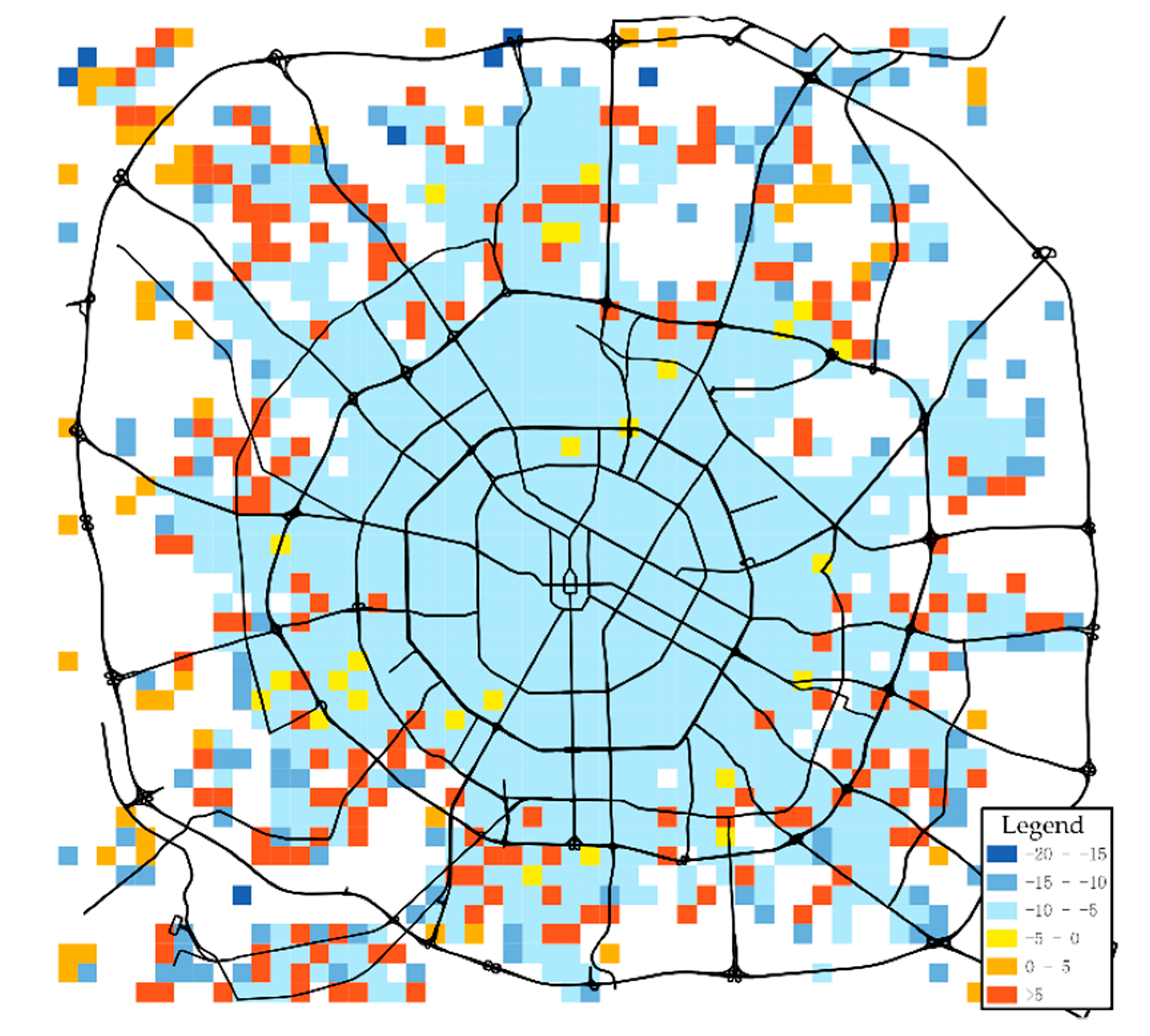
The difference scores of serving and idling at 18:00–18:10.

Figure 6.
The difference revenue between proposed method and compared method: (a) proposed method and random method; (b) proposed method and historic-based method; (c) proposed method and primary RL method; (d) proposed method and proposed method without expansion.
Figure 6.
The difference revenue between proposed method and compared method: (a) proposed method and random method; (b) proposed method and historic-based method; (c) proposed method and primary RL method; (d) proposed method and proposed method without expansion.


Figure 7.
The evaluated indicators in different scenarios: (a) the answer rate; (b) the total revenue; (c) the waiting time.
Figure 7.
The evaluated indicators in different scenarios: (a) the answer rate; (b) the total revenue; (c) the waiting time.


Table 1.
Notations.
| Variable | Explanation |
|---|---|
| S | An infinite state space |
| A | An infinite action space |
| P | A state transition probability matrix |
| R | Reward function |
| γ | A discount factor |
| s | State |
| s’ | Next State |
| a | Action |
| K | The time of the end state |
| The probability of taking action a at state s | |
| State value function | |
| State-action value function | |
| T | Time Space |
| L | Location Space |
| l | Location index of current state |
| l’ | Location index of next state |
| t | Time index of current state |
| t’ | Time index of next state |
| r | Order price |
| The reward when considering γ | |
| The reward of taking action a at state s | |
| Tr | Consuming number of transition steps on an order trip |
| α | Learning rate |
| Time difference |
Table 2.
Simulated results.
| Metric | Answer Rate | Total Revenue | Waiting Time(s) |
|---|---|---|---|
| Random method | 88.75% | 579,205.05 | 220 |
| Historic-based method | 89.35% | 582,295.24 | 220 |
| Primary RL method | 69.09% | 458,538.14 | 426 |
| Proposed RL method without expansion | 91.90% | 603,177.23 | 164 |
| Proposed RL method | 93.01% | 615,114.25 | 160 |
Table 3.
Simulated results using the relative percentage.
| Metric | Answer Rate% | Total Revenue% | Waiting Time(s)% |
|---|---|---|---|
| Random method | +4.80% | +6.20% | −27.27% |
| Historic-based method | +4.10% | +5.64% | −27.27% |
| Proposed RL method without expansion | +1.21% | +1.98% | −2.44% |
Publisher’s Note: MDPI stays neutral with regard to jurisdictional claims in published maps and institutional affiliations. |
© 2020 by the authors. Licensee MDPI, Basel, Switzerland. This article is an open access article distributed under the terms and conditions of the Creative Commons Attribution (CC BY) license (http://creativecommons.org/licenses/by/4.0/).
Share and Cite
MDPI and ACS Style
Jin, K.; Wang, W.; Hua, X.; Zhou, W. Reinforcement Learning for Optimizing Driving Policies on Cruising Taxis Services. Sustainability 2020, 12, 8883. https://0-doi-org.brum.beds.ac.uk/10.3390/su12218883
AMA Style
Jin K, Wang W, Hua X, Zhou W. Reinforcement Learning for Optimizing Driving Policies on Cruising Taxis Services. Sustainability. 2020; 12(21):8883. https://0-doi-org.brum.beds.ac.uk/10.3390/su12218883
Chicago/Turabian StyleJin, Kun, Wei Wang, Xuedong Hua, and Wei Zhou. 2020. "Reinforcement Learning for Optimizing Driving Policies on Cruising Taxis Services" Sustainability 12, no. 21: 8883. https://0-doi-org.brum.beds.ac.uk/10.3390/su12218883
Note that from the first issue of 2016, this journal uses article numbers instead of page numbers. See further details here.