Does the Environmental Kuznets Curve Exist? An International Study

Abstract

This study aims to examine the relationship between economic development and environmental degradation based on the Environmental Kuznets Curve (EKC) hypothesis. The level of CO₂ emissions is used as the indicator of environmental damage to determine whether or not greater economic growth can lower environmental degradation under the EKC hypothesis. The investigation was performed on eight major international economic communities covering 44 countries across the world. The relationship between economic growth and environmental condition was estimated using the kink regression model, which identifies the turning point of the change in the relationship. The findings indicate that the EKC hypothesis is valid in only three out of the eight international economic communities, namely the European Union (EU), Organization for Economic Co-operation and Development (OECD), and Group of Seven (G7). In addition, interesting results were obtained from the inclusion of four other control variables into the estimation model for groups of countries to explain the impact on environmental quality. Financial development (FIN), the industrial sector (IND), and urbanization (URB) were found to lead to increasing CO₂ emissions, while renewable energies (RNE) appeared to reduce the environmental degradation. In addition, when we further investigated the existence of the EKC hypothesis in an individual country, the results showed that the EKC hypothesis is valid in only 9 out of the 44 individual countries.

1. Introduction

Since the Industrial Revolution in the early 19th century, the manufacturing sector has become the main driver of economic development in many countries. The use of machinery and technological inputs in the production process has made a remarkable and profound change in the economic activities of people in the once agrarian societies, resulting in unprecedentedly rapid economic growth. However, industrially based economic growth has given rise to environmental degradation problems, and the combination of industrial activities has been a major contributor to global warming. According to the 2018 report of the Intergovernmental Panel on Climate Change (IPCC), the global average surface temperature increased by about 0.87 °C from the late 19th-century level, and climate and weather extremes have been found to occur more severely following the rise of global temperature by 0.5 °C These problems are caused by the greenhouse gases released from anthropogenic activities, which exert ecological and environmental impacts in the forms of more vagarious weather, greater severity of natural disasters, extreme drought in many regions, rising sea levels due to melting of polar ice caps, mutation and extinction of some living species, and impaired human health [1].

However, the Environmental Kuznets Curve (EKC) hypothesis on the relationship between income per capita and environmental degradation posits that, in its early stages, economic growth will be environmentally detrimental due to the increase in economic activities [2], but later, when the economy develops to a proper level, the previous environmental quality will be restored, indicating that the nexus of growth and the environment has a turning point. The EKC concept is a modified application of the Inverted-U Curve theory on the relationship between economic growth and income inequality by [3].

Recently, a plethora of research works have been produced to support the EKC theory, such as those by [4,5,6]. Although these studies use different variables and methods to estimate environmental degradation, their findings support the hypothesis that environmental degradation will level off as the economic development proceeds to the turning point. Nevertheless, many pieces of research came up with findings to reject the EKC theory, such as the works of [7,8,9], who did not find—and thus doubted—the U-curve relationship between economic growth and environmental degeneration.

As CO₂ is the primary greenhouse gas emitted from human activities, accounting for 76% of the total emission [10], many research attempts based on the EKC theory used CO₂ emissions as the variable indicating the level of environmental damage, such as in the works of [11,12]. However, some research works in the past demonstrated that the release of CO₂ is a function of many factors other than income and economic growth. For example, financial development through domestic credit provision was found to affect CO₂ emissions in both negative and positive directions. When the domestic credit widens the financial access by firms that have a mission to develop environmentally friendly technology or produce environmentally friendly products, it helps reduce future environmental degradation. On the contrary, financial development in favor of economic growth alone can increase CO₂ emissions [13,14]. Furthermore, a national economy’s industrialization was found to elevate CO₂ emissions both directly and indirectly due to energy use in the industrial production process and intensive energy consumption in other sectors following the economic growth and urbanization process [15].

Therefore, this research’s main objective is to validate the existence of the EKC in various economies in the world. Selected for the investigation are eight international economic communities, including the Association of Southeast Asian Nations (ASEAN), European Free Trade Association (EFTA), European Union (EU), Group of Seven (G7), Gulf Cooperation Council (GCC), Mercosur, North American Free Trade Agreement (NAFTA), and Organization for Economic Co-operation and Development (OECD), to further understand whether or not the different socio-political contexts and economic structures of the different countries or economic blocks have implications for the existence of the EKC and the relationship between economic growth and environmental quality. The existence of the EKC hypothesis is also examined at the individual country level as a robustness check. We want to note that these selected economic communities (or 44 countries) account for more than 90% of the world’s GDP and population. Apart from testing the validity of the EKC hypothesis, this study also has a secondary objective to assess other variables’ impacts beyond the economic growth on the extent of CO₂ emissions.

Consequently, to test the EKC hypothesis, this study proposes employing the kink regression model for fitting the data, as it can directly capture the nonlinear relationship between economic growth and environmental quality without the need for transforming the data into the quadratic form, as commonly employed in previous works [2,16,17,18]. The present authors believe that the quadratic function’s estimation is associated with overly distorted data, and the estimated result might not reflect the proper relationship between economic growth and environmental quality. Although the importance of the EKC hypothesis has been identified, the quadratic function is usually assumed in [11,12,17,18,19]. This paper calls into question the quadratic function assumption using time-series kink regression and panel kink regression for 1980−2016 in 44 countries within eight international economic communities, and it tests whether the results at the country level hold for different communities as a robustness check.

This paper is organized into six sections. Section 1 is the introduction, which provides the background and the significance of the study with the EKC. Section 2 reviews the EKC literature, related studies, and the factors affecting CO₂ emission levels, and describes the EKC theory. Section 3 deals with the concept of the kink regression model. Section 4 describes the data and variables used in the study. The main study findings are presented in Section 5. Section 6 gives conclusions and recommendations.

2. Related Theories and Research Works

2.1. The Environmental Kuznets Curve (EKC) Hypothesis

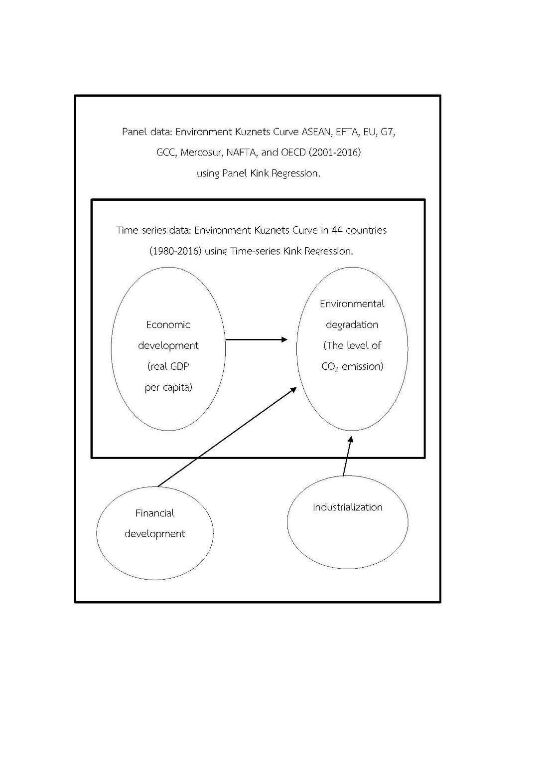
The Environmental Kuznets Curve (EKC) hypothesis explains an inverted U-shaped relationship between economic growth and environmental degradation (Figure 1), i.e., environmental pressure increases in the early stages of economic growth due to the increased release of pollutants and the extensive and intensive exploitation of natural resources associated with the greater use of production resources and the adoption of certain production technologies for the growing economic activities, up to a certain level, as income rises; and after that, it decreases, probably because of the growing public awareness and concern about environmental degradation and the research and development activities being oriented more toward the concept of the green economy when GDP grows at a high level [20,21].

2.2. Research Works on Testing the Existence of the EKC

Grossman and Krueger [2] examined the impact of NAFTA on the environment, considering the ambient concentrations of sulfur dioxide (SO₂) and suspended particulate matter (SPM) as the measures of environmental quality. They found a U-shaped relationship between GDP per capita and the two pollutants, which supports the Environmental Kuznets Curve (EKC) hypothesis. After this study, voluminous research works have been undertaken to validate the EKC theory using various econometric models and variables to measure the environmental condition. In the EKC literature, the environmental degradation is usually measured by the level of some pollutants, such as the commonly used CO₂ emissions, as found in the studies of Sinha and Shahbaz [12] for India, Pata [22] for Turkey, and Ahmad, Du, Lu, Wang, Li, Muhammad, and Hashmic [19] for Croatia. These three studies employed the Autoregressive Distributed Lag (ARDL) model to test the EKC hypothesis. Bekhet and Othman [17] recently conducted a causality test on the relationship between CO₂ emissions and GDP growth in Malaysia to confirm the EKC hypothesis. Some scholars obtained mixed results concerning the existence of the EKC, such as Shahbaz, Solarin, and Ozturk [16] who used the ARDL model for an investigation of 19 African countries, and found the EKC phenomenon to take place in only six countries, namely Algeria, Cameroon, the Congo Republic, Morocco, Tunisia, and Zambia; Atasoy [11] employed two methods to test the EKC hypothesis across the 50 states of the USA and found the Augmented Mean Group (AMG) method to provide supporting evidence in 30 states, while the use of the Common Correlated Effects Mean Group Estimator (CCEMG) indicated that the EKC hypothesis held in only 10 states. Aruga [18] examined the EKC hypothesis in the Asian-Pacific region using panel regression and cointegration models. He revealed that the hypothesis holds for the high-income group. Finally, the existence of the EKC hypothesis was also confirmed in emerging Eastern European and Central Asian countries [23].

However, some research works did not find the existence of the EKC in some countries. Pal and Mitra [24] used the ARDL model to examine the relationship between GDP per capita and CO₂ emissions in India and China, and their result indicated the presence of the N-shaped EKC, as the CO₂ emissions first increased at a greater rate than GDP growth and then decreased as the economic activities expanded, but stopped decreasing at a threshold before increasing again. Mikayilov, Galeotti, and Hasanov [25] studied the association between economic growth and CO₂ emissions in Azerbaijan using the Autoregressive Distributed Lag Bounds Testing (ARDLBT), Fully Modified Least Squares (FMOLS), Dynamic Least Squares (DOLS), and Canonical Cointegrating Regression (CCR) methods, which provided consistent findings that economic growth has a positive relationship with CO₂ emissions in the form of a monotonically increasing function in the long run, implying that the EKC hypothesis does not hold for Azerbaijan. Moutinho, Varum, and Madaleno [26] tested the EKC hypothesis for Spain and Portugal using data of 13 major economic sectors with Gross Value Added (GVA) representing income and the CO₂ emissions reflecting environmental degradation for an analysis by the Panel Corrected Standard Errors (PCSE) method. They found evidence of the N-shaped relationship between GVA and CO₂ emissions for Portugal and both N-shaped and inverted N-shaped functions for Spain. This means that there is a departure from the theoretical EKC because the CO₂ appeared to be reduced for a period, and then increase and decrease again along the path of GVA growth.

2.3. Factors Affecting the Levels of CO₂ Emissions

Some previous studies also paid attention to other explanatory variables of the extent of CO₂ emissions—for example, financial development, which helped lower CO₂ emissions in Malaysia and South Africa because it opened the opportunities for various business firms to gain access to more financial capital for investment in research and development of clean technologies [13,27]. However, financial development was found to promote CO₂ emissions in some countries. Pata [14] and Boutabba [28], for example, provided empirical evidence of the positive relationship between financial development and environmental degradation in Turkey and India, respectively. Furthermore, the industrialization process was found to link positively with the CO₂ emissions in China and Turkey due to the increased energy consumption for production activities in the manufacturing industry [15,22].

Furthermore, the literature also revealed that urbanization and renewable energy consumption also play an essential role in CO₂ emissions. Bilgili, Koçak, and Bulut [29] and Saidi and Omri [30] analyzed the link between renewable energy consumption and CO₂ emissions and reached similar results. Bilgili, Koçak, and Bulut [29] revisited the EKC hypothesis with the potential impact of renewable energy consumption on environmental quality. They found that renewables negatively impacted CO₂ emissions in seven OECD countries over the periods 1977−2010. In addition, Bhattacharya, Churchill, and Paramati [31] investigated the impact of renewable energies on environmental degradation in various economic regions and confirmed the harmful effects of renewable energies on emissions. These studies mentioned that a region could achieve a sustainable environment by discouraging fossil fuel energy generation and supporting clean energies, such as wind, solar, biomass, and geothermal energy sources. Urbanization was found to enhance carbon emissions by many previous studies (see [22,32,33]). People move to cities mainly because there are more employment opportunities in cities. Due to urbanization, the number of vehicles increases, and this affects traffic emissions.

In a nutshell, the empirical literature on the EKC theory’s validity cannot confirm that economic growth will eventually lead to improved environmental quality in the long run across all economies. The different methods used in the investigation can give different results to determine whether the EKC hypothesis holds for a particular country. Meanwhile, some research works did not take into account other crucial independent variables, like financial development and the structural change from such an economy as an agrarian-based to an industrialized/urbanized nation, which gives rise to different scales and directions of the environmental impacts across different economies. To fill these gaps, we have conducted a comparative empirical study to examine the EKC hypothesis in 44 individual countries worldwide and eight major international economic communities to produce a more precise idea on this issue. In addition, based on the reviewed literature, most previous studies examine the EKC using either the quadratic regression or panel quadratic regression; however, the quadratic function can bring severe problems with the determination of a model type and does not reflect the real non-relationship between dependent and independent variables [34]. Therefore, our study applies both time-series kink regression and panel kink regression models to test the EKC. We also investigate whether the kink regression and panel kink regression models have an advantage compared to the classical linear regression models.

3. Methodology

To perform the analysis in this study, we proceed as follows: First, the unit root test is undertaken for our variables. Second, we examine the existence of the EKC in the context of individual countries and each group of countries using the kink test of Hansen [35]. We note that 44 countries are considered in this study, and these countries can be classified into eight groups or regional markets, consisting of ASEAN, EFTA, EU, G7, GCC, Mercosur, NAFTA, and OECD. Third, the time-series kink regression and panel kink regression models are used to investigate the impact of economic development on the CO₂ emissions for individual countries and groups of countries, respectively.

3.1. Time-Series Kink Regression Model

Kink regression was proposed in 2017 by Hansen [35]. The model was introduced to explain the nonlinear relationship between each independent variable and the dependent variable. This model’s function is continuous, but its slope has a discontinuity at the kink or turning point. The structure of the model takes the following form:

$$Y_t={\beta }_0+{\beta }_1^{-}{(X_t-\gamma )}_{-}+{\beta }_1^{+}{(X_t-\gamma )}_{+}+e_t$$

(1)

where $Y_t$ is the dependent variable at time t, $X_t$ is the independent variable at time t, and $e_t$ denotes the error at time t. The parameters ${\beta }_0$, ${\beta }_1^{-}$, and ${\beta }_1^{+}$ are the constant term, the coefficient of ${(X_t-\gamma )}_{-}$, and the coefficient of $X_t$ ${(X_t-\gamma )}_{+}$, respectively. Note that $X_t$ is divided into two parts: a negative part,${(X_t-\gamma )}_{-}=\min (X_t-\gamma ,0)$, and a positive part, ${(X_t-\gamma )}_{+}=\max (X_t-\gamma ,0)$. In other words, ${(X_t-\gamma )}_{-}$ can be understood as $X_t\le \gamma$, while ${(X_t-\gamma )}_{+}$ refers to $X_t>\gamma$. The parameter $\gamma$ is called the kink point or turning point. To estimate all the unknown parameters of this model, we use the least squares estimation as follows:

$$\stackrel{⌢}{\mathsf{\beta }}(\gamma )=\underset{\mathsf{\beta }}{\arg \min }{\displaystyle \sum _{t=1}^T{(Y_t-{\beta }_0-{\beta }_1^{-}{(X_t-\gamma )}_{-}-{\beta }_1^{+}{(X_t-\gamma )}_{+})}^2}$$

(2)

This loss function is quadratic in $\mathsf{\beta }=\left\{{\beta }_0,{\beta }_1^{-},{\beta }_1^{+}\right\}$ but non-convex in $\gamma$. Hence, it is convenient to use a combination of concentration and grid search, such as:

$$\stackrel{⌢}{\gamma }=\underset{\gamma }{\arg \min } \underset{\mathsf{\beta }}{\min }\stackrel{⌢}{\mathsf{\beta }}(\gamma )$$

(3)

where $\stackrel{⌢}{\mathsf{\beta }}(\gamma )$ are the least-square coefficients given the candidate $\gamma$. The solution to Equation (3) can be found numerically through a grid search over $\gamma$. Once the optimal $\stackrel{⌢}{\gamma }$ is found, we can obtain the $\stackrel{⌢}{\mathsf{\beta }}$ using the least squares of $Y_t$ on ${(X_t-\stackrel{⌢}{\gamma })}_{-}$ and ${(X_t-\stackrel{⌢}{\gamma })}_{+}$. This study will build the time-series kink regression model on the basis of the EKC hypothesis. Thus, we need to rewrite Equation (1) in the following form.

$${\mathrm{lnCO}}_2{}_t={\beta }_o+{\beta }_1^{-}({\mathrm{lnGDPC}}_t-\gamma )+{\beta }_1^{+}({\mathrm{lnGDPC}}_t-\gamma )+e_t$$

(4)

where ${\mathrm{CO}}_2{}_t$ is the level of CO₂ emissions, and ${\mathrm{GDPC}}_t$ is the real gross domestic product per capita. To examine the existence of the EKC, we can consider the signs of ${\beta }_1^{-}$ and ${\beta }_1^{+}$. In accordance with our model, the negative sign of ${\beta }_1^{-}$ and positive sign of ${\beta }_1^{+}$ confirm the hypothesis of the existence of the EKC.

3.2. Panel Kink Regression Model

This study also investigates the existence of the EKC in groups of countries. Thus, the panel data of each group of countries are constructed and the panel kink regression model is used to fit these data. The model can be expressed as:

$$Y_{it}={\beta }_0+{\beta }_1^{-}{(X_{it}-\gamma )}_{-}+{\beta }_1^{+}{(X_{it}-\gamma )}_{+}+{\beta }_2{Z}_{it}+{\alpha }_i+e_{it},$$

(5)

where $Y_{it}$ and $X_{it}$ are, respectively, the dependent and independent variables of country i at time t. $Z_{it}$ is the $k\times 1$ vector of regressor ${\alpha }_i$ representing the individual effect of each country, and $e_{it}$ is the residual term of country i at time t. To estimate this model, we follow the fixed effect (F.E.) estimation method proposed by Zhang, Zhou, and Jiang [36]. As ${\alpha }_i$ is not observable, we then eliminate ${\alpha }_i$ by demeaning the variables using the within transformation.

Thus, we can transform our variables as follows:

$${\tilde{Y}}_{it}=Y_{it}-\frac{1}{T}{\displaystyle \sum _{t=1}^T{Y}_{it}}$$

(6)

$${\tilde{X}}_{it}=\frac{1}{T}{\displaystyle \sum _{t=1}^T{X}_{it}^{}}$$

(7)

$${\tilde{Z}}_{it}=\frac{1}{T}{\displaystyle \sum _{t=1}^T{Z}_{it}}$$

(8)

$${\dot{\epsilon }}_{it}={\epsilon }_{it}-\frac{1}{T}{\displaystyle \sum _{t=1}^T{\epsilon }_{it}}$$

(9)

Then, we can rewrite our Panel model (Equation (5)) as

$${\tilde{Y}}_{it}={\beta }_0+{\beta }_1^{-}{({\tilde{X}}_{it}-\gamma )}_{-}+{\beta }_1^{+}{({\tilde{X}}_{it}-\gamma )}_{+}+{\beta }_2{\tilde{Z}}_{it}+{\tilde{e}}_{it}.$$

(10)

Then, we can use the F.E. estimation for estimating $\mathsf{\beta }=\left\{{\beta }_0,{\beta }_1^{-},{\beta }_1^{+},{\beta }_2\right\}$ and $\gamma$ by:

$$\tilde{\mathsf{\beta }}(\gamma )=\underset{\beta ,\gamma }{\arg \min }{\displaystyle \sum _{t=1}^T{\Vert {\tilde{Y}}_{it}-{\beta }_0-{\beta }_1^{-}{({\tilde{X}}_{it}-\gamma )}_{-}-{\beta }_1^{+}{({\tilde{X}}_{it}-\gamma )}_{+}-{\beta }_2{\tilde{Z}}_{it}\Vert }_{}^2}$$

(11)

Similar to the time-series kink regression, the loss function takes a quadratic form in $\mathsf{\beta }$, but is not differentiable with respect to $\gamma$. Again, we can apply the grid search to solve this minimization problem:

$$\stackrel{⌢}{\gamma }=\underset{\gamma }{\arg \min } {\displaystyle \sum _{t=1}^T{\Vert {\tilde{Y}}_{it}-{\tilde{\beta }}_0-{\tilde{\beta }}_1^{-}{({\tilde{X}}_{it}-\gamma )}_{-}-{\tilde{\beta }}_1^{+}{({\tilde{X}}_{it}-\gamma )}_{+}-{\tilde{\beta }}_2{\tilde{Z}}_{it}\Vert }_{}^2}$$

(12)

When the optimal $\stackrel{⌢}{\gamma }$ is obtained, we can obtain the optimal $\stackrel{⌢}{\mathsf{\beta }}(\stackrel{⌢}{\gamma })$.

In this study, we apply this panel kink regression to investigate the existence of the EKC in various economic groups. We also consider two additional economic factors as the control variables. Thus, our empirical model takes the form:

$${\mathrm{lnCO}}_2{}_{it}={\beta }_o+{\beta }_1^{-}({\mathrm{lnGDPC}}_{it}-\gamma )+{\beta }_1^{+}({\mathrm{lnGDPC}}_{it}-\gamma )+{\beta }_3{\mathrm{lnFIN}}_{it}+{\beta }_4{\mathrm{lnIND}}_{it}+{\beta }_5{\mathrm{lnURB}}_{it}+{\beta }_6{\mathrm{lnRNE}}_{it}+e_t$$

(13)

where ${\mathrm{FIN}}_{it}$ is the financial development factor, ${\mathrm{IND}}_{it}$ is the industrialization, ${\mathrm{URB}}_{it}$ is urbanization, and ${\mathrm{RNE}}_{it}$ is renewable energies. These variables are considered the control variables in this study. The discussion of the effects of these control variables on CO₂ is previously conducted in Section 2.

3.3. Testing for the Kink Effect

As we aim to determine whether the EKC exists in both individual countries and groups of countries, the nonlinear relationship between CO₂ and GDP per capita (GDPC) (or kink effect) is first investigated before obtaining the ${\beta }_1^{-}$ and ${\beta }_1^{+}$. If there is no presence of the kink effect, the relationship between CO₂ and GDPC is linear, and thus, we cannot fit our data using the kink regression model. To test the kink effect’s presence, we follow the F-statistic proposed in Hansen [35]. The null hypothesis of the kink effect and the alternative hypothesis of no kink effect (linear model) are as follows:

$$\begin{array}{l}{H}_0:{\beta }_1^{-}={\beta }_1^{+}\\ H_a:{\beta }_1^{-}\ne {\beta }_1^{+}.\end{array}$$

(14)

The test statistic is of the F-type:

$$F_T^{*}=\frac{T\left({\tilde{\sigma }}^2-{\stackrel{⌢}{\sigma }}^2\right)}{{\stackrel{⌢}{\sigma }}^2},$$

(15)

where ${\tilde{\sigma }}^2$ and ${\stackrel{⌢}{\sigma }}^2$ are the error variances of linear regression and kink regression, respectively. Given that there may exist a non-standard distribution of an F-statistic test, Hansen [35] suggested using a bootstrap method to produce the first-order asymptotic distribution for testing. He showed that a bootstrap procedure attains the first-order asymptotic distribution; thus, the p-values constructed from the bootstrap are asymptotically valid. Finally, we reject the null hypothesis if the bootstrapped p-value of this test is less than the critical value α. In other words, if the null hypothesis is rejected, there exists a nonlinear relationship between CO₂ and GDPC.

A similar procedure is replicated in testing the kink effect in the context of panel data. We note that the individual specific effects are removed from the panel data model using the mean differencing method, as presented in Section 3.2; hence, the kink effect testing presented above can be used for panel kink regression.

4. Data and Variables Used in the Study

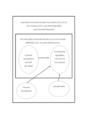
As permitted by the data availability, this study uses panel data of eight groups of countries, including EFTA, EU, G7, GCC, Mercosur, NAFTA, ASEAN, and OECD (Appendix A

Table A1. List of countries in each economic community.

Economic Group	List of Countries Considered in This Study
ASEAN	Brunei Darussalam, Indonesia, Malaysia, Philippines, Singapore, Thailand
NAFTA	Canada, Mexico, United States
GCC	Bahrain, Kuwait, Oman, Qatar, Saudi Arabia, United Arab Emirates
EFTA	Iceland, Norway, Switzerland
MERCOSUR	Argentina, Brazil, Paraguay, Uruguay
EU	Austria, Belgium, Bulgaria, Cyprus, Denmark, Finland, France, Greece, Italy, Luxembourg, Malta, Netherlands, Portugal, Ireland, Spain, Sweden
OECD	Australia, Austria, Belgium, Canada, Denmark, Finland, France, Greece, Iceland, Italy, Japan, Luxembourg, Mexico, Netherlands, New Zealand, Norway, Portugal, Ireland, Korea Republic, Spain, Sweden, Switzerland, Turkey, United Kingdom, United States
G7	Canada, France, Italy, Japan, United Kingdom, United States

), spans from 2001 to 2016, and uses carbon dioxide emissions (CO₂) as a proxy of environmental degradation and real GDP per capita as an indicator of economic development. Industrialization, financial development, urbanization, and renewable energies are also considered as the crucial variables (control variables) that affect CO₂ emissions and are included in this analysis. In addition, this study uses yearly time series data running from 1980 to 2016 of CO₂ emissions and real GDP per capita of 44 individual countries, which are member countries of the eight groups, including Argentina, Australia, Bahrain, Belgium, Brazil, Brunei, Bulgaria, Canada, Cyprus, Denmark, Finland, France, Greece, Indonesia, Iceland, Italy, Japan, Kuwait, Luxembourg, Mexico, Malta, Malaysia, the Netherlands, Norway, New Zealand, Oman, the Philippines, Portugal, Paraguay, Qatar, Ireland, Saudi Arabia, Singapore, South Korea, Spain, Sweden, Switzerland, Thailand, Turkey, the United Arab Emirates, the United Kingdom, the United States of America, and Uruguay.

We would like to note that our time series’ sample size is 36 observations, which would be enough to estimate time-series kink regression, as there are only four parameter estimates (see Equation (4)). Lee and Song [37] and Van De Schoot et al. [38] suggested that the frequentist estimation is still reliable when the sample size is equal to or larger than three times the parameters. As Muthén and Muthén [39] argued, the only way to answer the sample size question is by performing a simulation study. Fortunately, Tarkhamtham and Yamaka [40] provided a simulation study of the kink regression model’s and compared various estimation techniques. They showed that the least squares could produce a reliable kink regression estimation result (four parameter estimates) and low bias when the simulated data sample size is 20.

Table 1. Description of variables.

Variable	Description	Symbol
Environmental Degradation	Environmental degradation is measured using territorial CO2 emissions, which come from the burning of fossil fuels due to human activities as well as production processes. This variable is considered a dependent variable in our analysis (unit: metric tons per capita).	CO2
Economic Development	Economic development in this analysis is measured by real GDP per capita, purchasing power parity (PPP) (2011 constant international dollars), which is the value of all goods and services produced by a country divided by the total population. This variable should produce a positive impact on environmental degradation in the early stage of development. Then, the impact should become negative according to the EKC hypothesis.	GDPC
Financial Development	Financial development is considered another explanatory variable in the analysis of groups of countries. This variable is measured by domestic credit to the private sector (% of GDP), which refers to the financial resources provided by financial corporations to the private sector.	FIN
Industrialization	Industrialization refers to the transformation from an agrarian-based to an industrialized economy. In this analysis, this variable is measured by the industry with value added (unit: % of GDP).	IND
Urbanization	The urban population refers to people living in urban areas as defined by national statistical offices. The data are collected and smoothed by the United Nations Population Division (unit: % of population).	URB
Renewable energies	Renewable energies include wind, solar, biomass, and geothermal energy sources. This means all energy sources that renew themselves within a short time or are permanently available. Renewable energy is measured as a share in final energy consumption (unit: % of energy consumption).	RNE

describes the variables used in the study.

In this study, both panel data and time-series data are considered to investigate the EKC hypothesis for eight major international economic communities and the 44 countries within their communities, respectively. We thus perform both the Levin, Lin, and Chu (LLC) unit root test for panels [41] and the Augmented Dicky–Fuller (ADF) unit root test for time-series [42] to analyze the stationarity of the data. After passing the stationarity test, the data can be used for estimation by the kink regression model. This study consists of two main parts: (1) testing the EKC hypothesis for each of the eight major groups of countries, namely EFTA, EU, G7, GCC, Mercosur, NAFTA, ASEAN, and OECD, taking into account the effects of financial development and the significance of the industrial sector, urbanization, and renewable energies on the level of CO₂ emissions; (2) testing the EKC hypothesis for 44 individual countries worldwide in order to test, for each country, whether or not a kink point exists in the relationship between its income per capita and environmental degradation.

Before using the panel data and time-series data for the kink regression model estimation, this study ran a unit root test to find out whether the data sets are stationary. The test results are presented in

Table 2. Results of the time-series Augmented Dicky–Fuller (ADF) unit root test.

lnGDPC
Country	I(0)	I(1)	Country	I(0)	I(1)	Country	I(0)	I(1)
Argentina	−1.020	−4.832 ***	Iceland	−1.122	−5.938 ***	Qatar	−2.029	−10.288 ***
Australia	−0.938	−3.232 ***	Italy	−0.433	−2.292 *	Ireland	−1.021	−7.287 ***
Austria	−0.8723	−2.973 **	Japan	−0.323	−2.928 **	Saudi Arabia	−0.983	−4.092 ***
Bahrain	−1.233	−3.088 ***	Kuwait	−1.672	−4.221 ***	Singapore	−1.088	−5.982 ***
Belgium	−1.221	−5.932 ***	Luxembourg	−1.121	−9.383 ***	South Korea	−1.092	−5.109 ***
Brazil	−0.992	−4.233 ***	Mexico	−0.887	−5.393 ***	Spain	−0.133	−3.091 **
Brunei	−0.322	−3.099 ***	Malta	−0.232	−2.977 **	Sweden	−0.283	−4.002 ***
Bulgaria	−0.221	−4.988 **	Malaysia	−0.905	−6.943 ***	Switzerland	−0.863	−4.211 ***
Canada	−1.221	−6.988 ***	Netherland	−2.001	−5.032 ***	Thailand	−1.622	−6.993 ***
Cyprus	−0.672	−2.938 **	Norway	−1.983	−8.937 ***	Turkey	−1.032	−5.039 ***
Denmark	−1.028	−6.093 ***	New Zealand	−1.221	−4.083 ***	UAE	−1.082	−6.223 ***
Finland	−0.988	−3.329 **	Oman	−0.637	−6.993 ***	UK	−0.382	−4.001 ***
France	−1.228	−5.022 ***	Philippines	−0.082	−5.982 ***	US	−0.221	−3.902 ***
Greece	−0.232	−2.383 *	Portugal	−0.234	−3.023 **	Uruguay	−0.673	−5.093 ***
Indonesia	−1.872	−6.093 ***	Paraguay	−1.722	−5.938 ***		−1.001	−5.221 ***
lnCO2
Country	I(0)	I(1)	Country	I(0)	I(1)	Country	I(0)	I(1)
Argentina	−0.883	−3.092 **	Iceland	−0.983	−5.101 ***	Qatar	−1.872	−8.983 ***
Australia	−0.212	−3.121 **	Italy	−1.090	−6.002 ***	Ireland	−0.882	−3.831 **
Austria	−0.129	−3.011 **	Japan	−2.011	−7.155 ***	Saudi Arabia	−0.362	−3.991 **
Bahrain	−0.881	−4.920 ****	Kuwait	−0.728	−4.920 ***	Singapore	−1.009	−4.027 ***
Belgium	−1.021	−6.001 ***	Luxembourg	−3.928	−5.219 **	South Korea	−0.628	−4.982 ***
Brazil	−0.122	−3.221 **	Mexico	−0.221	−3.292 **	Spain	−0.512	−4.778 ***
Brunei	−0.312	−3.423 **	Malta	−0.449	−3.982 ***	Sweden	−0.398	−3.982 ***
Bulgaria	−0.622	−4.221 ***	Malaysia	−0.983	−4.772 ***	Switzerland	−0.447	−4.002 ***
Canada	−2.001	−7.930 ***	Netherland	−1.593	−6.112 ***	Thailand	−1.921	−6.766 ***
Cyprus	−0.392	−3.120 **	Norway	−1.335	−6.029 ***	Turkey	−0.223	−3.652 **
Denmark	−1.122	−5.550 ***	New Zealand	−0.873	−4.832 ***	UAE	−1.982	−6.871 ***
Finland	−0.526	−3.212 **	Oman	−0.234	−5.032 ***	UK	−0.293	−3.521 **
France	−0.219	−4.020 ***	Philippines	−0.882	−3.028 ***	US	−1.773	−7.938 ***
Greece	−0.110	−3.921 ***	Portugal	−0.432	−2.893 **	Uruguay	−0.673	−3.229 **
Indonesia	−2.091	−7.993 ***	Paraguay	−1.001	−4.389 ***		−1.012	−5.039 ***

Note: “*”, “**”, and “***” indicate statistical significance at the 0.05, 0.01, and 0.001 levels, respectively.

and

Table 3. Results of the panel Levin, Lin, and Chu (LLC) unit root test.

	G7	OECD	EU	Mercosur
lnCO2	−2.843 **	−3.722 **	−3.219 **	−4.013 ***
lnGDPC	−3.432 **	−4.743 ***	−3.414 **	−3.122 **
lnFIN	−4.651 ***	−7.552 ***	−7.068 ***	−7.382 ***
lnIND	−4.556 ***	−4.923 ***	−5.893 **	−4.323 ***
lnURB	−3.232 **	−2.938 **	−3.232 **	−4.883 ***
lnRNE	−3.092 **	−5.333 ***	−3.738 ***	−3.422 **
	EFTA	GCC	NAFTA	ASEAN
lnCO2	−3.222 **	−3.216 **	−3.563 **	−3.014 **
lnGDPC	−4.361 ***	−5.922 ***	−2.952 **	−3.532 **
lnFIN	−4.245 ***	−5.234 ***	−3.565 **	−4.654 ***
lnIND	−3.208 **	−4.897 ***	−4.178 ***	−5.136 ***
lnURB	−3.543 **	−3.118 **	−4.513 ***	−4.432 ***
lnRNE	−2.983 **	−4.232 ***	−3.901 **	−4.221 ***

Note: “*”, “**”, and “***” indicate statistical significance at the 0.05, 0.01, and 0.001 levels, respectively.

, respectively, for the ADF test and LLC test. It can be seen that all panel variable series of all groups of countries are stationary, as the corresponding p-values are less than 0.05, leading to the rejection of the null hypothesis that the variable is non-stationary or possesses a unit root. Thus, these panel datasets can be used for panel kink regression estimation. However, in the case of time-series data, the ADF test is performed for time series of individual countries; it is found that the lnCO₂ and lnGDC variables of all countries are stationary at the first difference.

5. Empirical Results

5.1. Investigating the EKC Hypothesis for Groups of Countries

Before testing the EKC hypothesis using the F-test as described in Section 3.3, it is necessary to test for the existence of a kink point in the kink regression to confirm that the structural relationship between the independent variable and the dependent variable is nonlinear using the F-test.

In addition to merely examining the influence of economic growth on the environmental quality, the researchers determined to take into account other variables that can play roles in driving the increase or decrease of CO₂ emissions, namely the factors of financial development (FIN), the prominence of the industrial sector (IND), urbanization (URB), and renewable energies (RNE), as expressed in a full relationship by Equation (13).

According to F-test in

Table 4. Results of the F-test for the kink effects for eight major groups of countries.

Group	${\mathit{F}}_{\mathit{T}}^{*}$
ASEAN	116.938 ***
NAFTA	129.332 ***
GCC	132.938 ***
EFTA	118.672 ***
MERCOSUR	113.123 ***
EU	110.221 ***
OECD	122.323 ***
G7	129.009 ***

Note: “***” indicates that the country has a nonlinear relationship between its CO₂ emissions and GDP per capita (GDPC) with the presence of a kink effect at the 0.001 level of statistical significance.

, we can observe that the null hypothesis of the kink effect is rejected at the 5% statistical level in all groups of countries, indicating that the CO₂–GDPC nexus is nonlinear. Hence, the following panel kink regression analysis is suitable for investigating the EKC’s existence.

5.2. Estimation Results from the Panel Kink Regression Model

Table 5. Parameter estimates from the panel kink regression model for eight groups of countries.

Dependent variable: territorial CO2 emissions (lnCO2)
		Coefficient	S.E.
ASEAN	lnGDPC $\le$ 9.473	0.801 **	0.184
	lnGDPC $>$ 9.473	−0.273	0.322
	lnFIN	0.131	0.281
	lnIND	0.015	0.011
	lnURB	0.823 ***	0.213
	lnRNE	−0.003	0.002
NAFTA	lnGDPC $\le$ 10.204	−0.412 *	0.201
	lnGDPC $>$ 10.204	−1.132 ***	0.187
	lnFIN	0.218 *	0.100
	lnIND	0.043 **	0.012
	lnURB	0.321	0.221
	lnRNE	−0.002 *	0.001
GCC	lnGDPC $\le$ 10.123	0.389	0.312
	lnGDPC $>$ 10.123	0.633 ***	0.135
	lnFIN	0.223 ***	0.010
	lnIND	0.256 **	0.091
	lnURB	0.563 ***	0.112
	lnRNE	−0.012	0.021
EFTA	lnGDPC $\le$ 11.244	−1.152 **	0.39
	lnGDPC $>$ 11.244	−1.009 *	0.47
	lnFIN	0.212 *	0.100
	lnIND	0.182 ***	0.013
	lnURB	0.232	0.201
	lnRNE	−0.006 **	0.002
Mercosur	lnGDPC $\le$ 8.783	0.782 *	0.310
	lnGDPC $>$ 8.783	0.891 ***	0.192
	lnFIN	0.221	0.151
	lnIND	0.532 *	0.201
	lnURB	0.553 ***	0.151
	lnRNE	−0.001	0.001
EU	lnGDPC $\le$ 10.465	0.389 ***	0.108
	lnGDPC $>$ 10.465	−0.211 ***	0.073
	lnFIN	0.122 ***	0.031
	lnIND	0.149 ***	0.051
	lnURB	0.123 ***	0.032
	lnRNE	−0.033 *	0.015
OECD	lnGDPC $\le$ 10.542	0.477 ***	0.120
	lnGDPC $>$ 10.542	−0.465 **	0.132
	lnFIN	0.121 *	0.053
	lnIND	0.321 ***	0.101
	lnURB	0.232	0.214
	lnRNE	−0.006 ***	0.002
G7	lnGDPC $\le$ 10.721	1.224 *	0.502
	lnGDPC $>$ 10.721	−1.832 ***	0.642
	lnFIN	0.323 *	0.123
	lnIND	0.062 ***	0.009
	lnURB	0.019 ***	0.002
	lnRNE	−0.030 **	0.010

Note: “*”, “**”, and “***” indicate statistical significance at the 0.05, 0.01, and 0.001 levels, respectively. S.E. denotes standard error.

displays the parameter estimates from the panel kink regression model for groups of countries.

The estimation results displayed in Table 5 indicate that the EKC hypothesis holds in the EU, OECD, and G7 communities, as the levels of CO₂ emissions are high at the early stages of economic growth (lnGDPC $\le$ $\gamma$ has a positive slope), but the emissions declined with the economic growth beyond the turning point (lnGDPC $>$ $\gamma$ has negative slope). In the case of the EU, when the lnGDPC remain below 10.465, the increase of GDPC by 1% results in an increase in the level of CO₂ emissions by 0.389%; but after the kink point with the lnGDPC greater than 10.465, a 1% increase in the real GDP per capita lead to the reduction of CO₂ emissions by 0.211%. Thus, the relationship between economic growth and environmental quality in the EU group is consistent with the EKC hypothesis. The same relationship also exists in other groups. In the OECD group, the increase in economic growth by 1% before reaching the kink point resulted in an increase in the level of CO₂ emissions by 0.477%, but a 1% increase in GDPC after passing the kink point at 10.542 brought about the massive decrease in CO₂ emissions by 0.465%, which is a rate of decrease 1.7 and 2.2 times greater compared to the ASEAN (−0.273) and EU (−0.211) groups, respectively. G7 is the group that produces the most CO₂ emissions among the eight groups of countries when its income per capita is lower than the kink point at 10.721, as a 1% increase in GDPC causes the CO₂ emissions to increase by as much as 1.224%; however, its economic development beyond the kink point led to an enormous reduction of CO₂ emissions by 1.832% given a 1% increase in GDPC. In the cases of NAFTA and EFTA, their economic development has gone hand in hand with the declining emissions. The NAFTA group, in particular, given a 1% increase in GDPC, before reaching the kink point at 10.204, can reduce CO₂ emissions by 0.412% and then by 1.132% when the economy grows beyond the kink point. On the contrary, the economic growth of the GCC and Mercosur groups proceeds with continuously rising CO₂ emissions. After passing the kink point at 10.123, the GCC group experienced an increase in CO₂ emissions by 0.633%. However, there is an insignificant effect of GDPC on CO₂ emissions before reaching their kink point (lnGDPC $\le$10.123). Meanwhile, a 1% increase in the GDPC of the Mercosur group in either the pre- or post-kink-point period has an association with an approximately 0.8% increase in CO₂ emissions.

For each group of countries found to have a relationship between economic growth and environmental degradation conforming to the EKC hypothesis, their real GDP per capita (USD) at the turning point, which should be maintained or pushed higher for environmental sustainability, can be obtained by transforming the corresponding kink point value into the exponential form. As shown in

Table 6. Estimated kink point values and the corresponding optimal real GDP per capita (USD) level for countries with the empirical Environmental Kuznets Curve (EKC).

	$\mathbf{Kink} \mathbf{Point} (\gamma )$	Real GDP Per Capita (USD)
EU	10.465	35,066.45
OECD	10.542	37,873.24
G7	10.721	45,297.18

Note: Real GDP per capita (USD) was obtained by converting the kink point value into the exponential form.

, for the EU, OECD, and G7 groups, the level of CO₂ emissions will decrease when the respective real GDP per capita level is equal to or higher than 35,066.45, 37,873.24, and 45,297.18 USD.

According to this panel analysis, the EKC hypothesis only stands for the EU, G7, and OECD, while it is not apparent for ASEAN-5, NAFTA, GCC, EFTA, or MERCOSUR. This indicates that the transition in the CO₂ emissions along the EKC is only occurring in the three developed economic groups (EU, G7, and OECD). The possible reason is that these developed groups may employ energy policies to enhance their energy efficiency. However, for emerging economic groups, economic development is probably their higher priority, rather than introducing more efficient energy sources to solve environmental degradation.

Moreover, it was found that the four additional control variables considered in the model also affected the level of CO₂ emissions in two directions. The coefficients of FIN, IND, and URB have a certain positive effect on CO₂ emissions; however, RNE is negative. FIN shows a significant and positive impact on CO₂ emissions for the NAFTA, GCC, EFTA, EU, OECD, and G7 groups because financial development widened the access to capital, thus making it attractive for private businesses to make the investment to expand industrial activities that also produced pollutants as by-products. This phenomenon is consistent with the previous research findings of Shahbaz, Hussain, Ahmad, and Alam [43], which indicated that financial development, particularly the greater access to financial sources, led to environmental degradation. In addition, the positive impact of financial development is also supported by the previous findings of the studies by Shahbaz et al. [44] for BRICS(Brazil, Russia, India, China and South Africa) and 11 post-transition European economies, Kilic and Balan [45] for 151 countries, Shoaib et al. [46] for G7 and eight developing countries, and Shahbaz, Tiwari, and Nasir [13] for South Africa. Halliru et al. [47] suggested that greater financial development is directed in favor of the industrial sector, particularly manufacturing and mining, resulting in increased pollution. When making a comparison among the coefficients of FIN on CO₂ emissions, we obtain the results that FIN’s coefficient of G7 is the highest with a value of 0.323, followed by the GCC (0.223), NAFTA (0.218), EFTA (0.182), EU (0.122), and OECD (0.121) groups. Meanwhile, the factor of IND, the importance of the industrial sector measured by its value-added share in GDP, is found to relate positively with the increase in CO₂ emissions in all groups of countries (except for ASEAN), probably because the investment in expansion of the industrial sector involved greater energy consumption in the production process, thus causing the CO₂ emissions to increase. Interestingly, the industrialization of ASEAN had an insignificant effect on CO₂ emissions. The possible reason is that the ASEAN group’s environmental rules and regulations are strict, and they are not emitting carbon. Moreover, the ASEAN industry sectors rely on soft industry, which is not a source of pollution [33].

Concerning urbanization (URB), it reveals that most of URB’s coefficients are statistically significant. The results indicate that URB’s coefficients for ASEAN, GCC, Mercosur, and G7 are positive and that carbon emission is elastic concerning urbanization; a 1% increase in urbanization increases carbon emissions within a range of 0.019% (G7) to 0.823% (ASEAN). Our findings are in line with those of Pata [14], Ali, Bakhsh, and Yasin [32], Saidi and Omri [30], and Zafar et al. [20]. Urbanization plays a more important role in ASEAN than in the other three groups. Rapid urbanization has occurred in ASEAN since its inception, and its pace has accelerated during recent decades. One of the main problems of this rapid urbanization is traffic emissions, which influence the environmental quality in urban areas. In the cases of NAFTA, EU, EFTA, and OECD, we found that urbanization has no significant impact on CO₂ emissions. We expect that green transportation development as public transportation in these groups is provided in the cities, thereby reducing energy consumption and harmful CO₂ emissions. Saidi and Omri [30] suggested that the improvement of green technology by urban industrial and residential sectors is provided to train and educate people regarding mitigation and adaptation with respect to environmental degradation.

Nevertheless, a significant negative relationship holds between renewable energies (RNE) and CO₂ emissions. The result shows that renewable energy consumption has a significant impact on carbon emissions for five groups out of the eight, meaning that carbon emissions are elastic with respect to renewable energy consumption. Particularly, the coefficient of renewables is negative and statistically significant for the NAFTA (−0.002), EFTA (−0.006), EU (−0.033), OECD (−0.006), and G7(−0.033) groups. This finding is consistent with those of Saidi and Omri [30], who also found a causality link from renewable energies to carbon emissions in various regions.

To have the robustness result, we compare the performance between panel kink regression and linear panel regression in the forms of both pooled data and fixed effects models based on the minimum Bayesian Information Criterion (BIC) to select the best model for estimation. From the calculated BICs presented in

Table 7. Calculated Bayesian Information Criterion (BIC) of various regression models.

	Panel Linear Regression		Panel Kink Regression
BIC	Pooled	Fixed	Pooled	Fixed
ASEAN	−28.098	−30.832	−30.772	−40.215
NAFTA	−13.982	−16.982	−29.001	−35.591
GCC	−14.662	−15.349	−17.110	−24.641
EFTA	−9.098	−10.221	−12.492	−23.955
MERCOSUR	−4.811	−13.092	−8.321	−16.022
EU	−9.451	−10.326	−12.984	−26.091
OECD	−3.921	−4.773	−5.223	−6.832
G7	−6.983	−8.983	−9.021	−20.332

Note: The lowest BIC values are presented in bold font.

, it can be seen that the panel kink regression model is consistently superior to the panel linear regression model across groups of countries for the relatively lower BIC values. Furthermore, for the estimation by two different approaches of panel data regression, it was found that the panel regression model in both kink and linear forms using the fixed effects approach is more suitable than that with the pooled data approach considering the lower BIC values across all groups of countries.

5.3. Investigating the EKC Hypothesis for Individual Countries

After having tested the EKC hypothesis for individual countries with the result confirming the existence of the EKC in some countries, the present researchers still had an interest in testing the nonlinear relationship between growth and emissions at the aggregate level focusing on the major international groups of economies. The results of the test for the kink effect for individual countries are presented in

Table 8. Results of the F-test for the kink effects for the 44 individual countries.

Country	${\mathit{F}}_{\mathit{T}}^{*}$	Country	${\mathit{F}}_{\mathit{T}}^{*}$	Country	${\mathit{F}}_{\mathit{T}}^{*}$
Argentina	5.291	Iceland	0.882	Qatar	4.585
Australia	10.302 ***	Italy	0.227	Ireland	7.930 *
Austria	7.938 **	Japan	0.921	Saudi Arabia	6.483 *
Bahrain	6.832 *	Kuwait	6.331 **	Singapore	6.355 *
Belgium	2.883	Luxembourg	0.821	South Korea	6.492 *
Brazil	2.123	Mexico	0.771	Spain	4.021
Brunei	4.981	Malta	1.872	Sweden	4.902
Bulgaria	1.321	Malaysia	4.324	Switzerland	5.022
Canada	1.673	Netherland	9.232 **	Thailand	4.999
Cyprus	5.301	Norway	11.282 ***	Turkey	6.883 *
Denmark	12.381 ***	New Zealand	10.992 ***	UAE	1.156
Finland	4.211	Oman	7.432 *	UK	10.982 ***
France	3.928	Philippines	1.239	US	1.090
Greece	1.992	Portugal	8.921 *	Uruguay	1.001
Indonesia	0.862	Paraguay	6.472 *

Note: “*”, “**”, and “***” indicate statistical significance at the 0.05, 0.01, and 0.001 levels, respectively. A statistically significant result means that the country has a nonlinear relationship between its CO₂ emissions and GDPC with the presence of a kink effect. In addition, as our time series data are stationary at I(1), our time series result may face the spurious regression problem. To clarify this problem, we take Engle’s and Granger’s cointegration test from Engle and Yoo [48] to examine the existence of the long-run relationship between the dependent and independent variables in the kink regression model. The result confirms the long-run nonlinear relationship between CO₂ emissions and GDPC (see Table A2).

, which shows that the nonlinear relationship between real GDP per capita and CO₂ emissions exists in 17 out of the 44 countries under study.

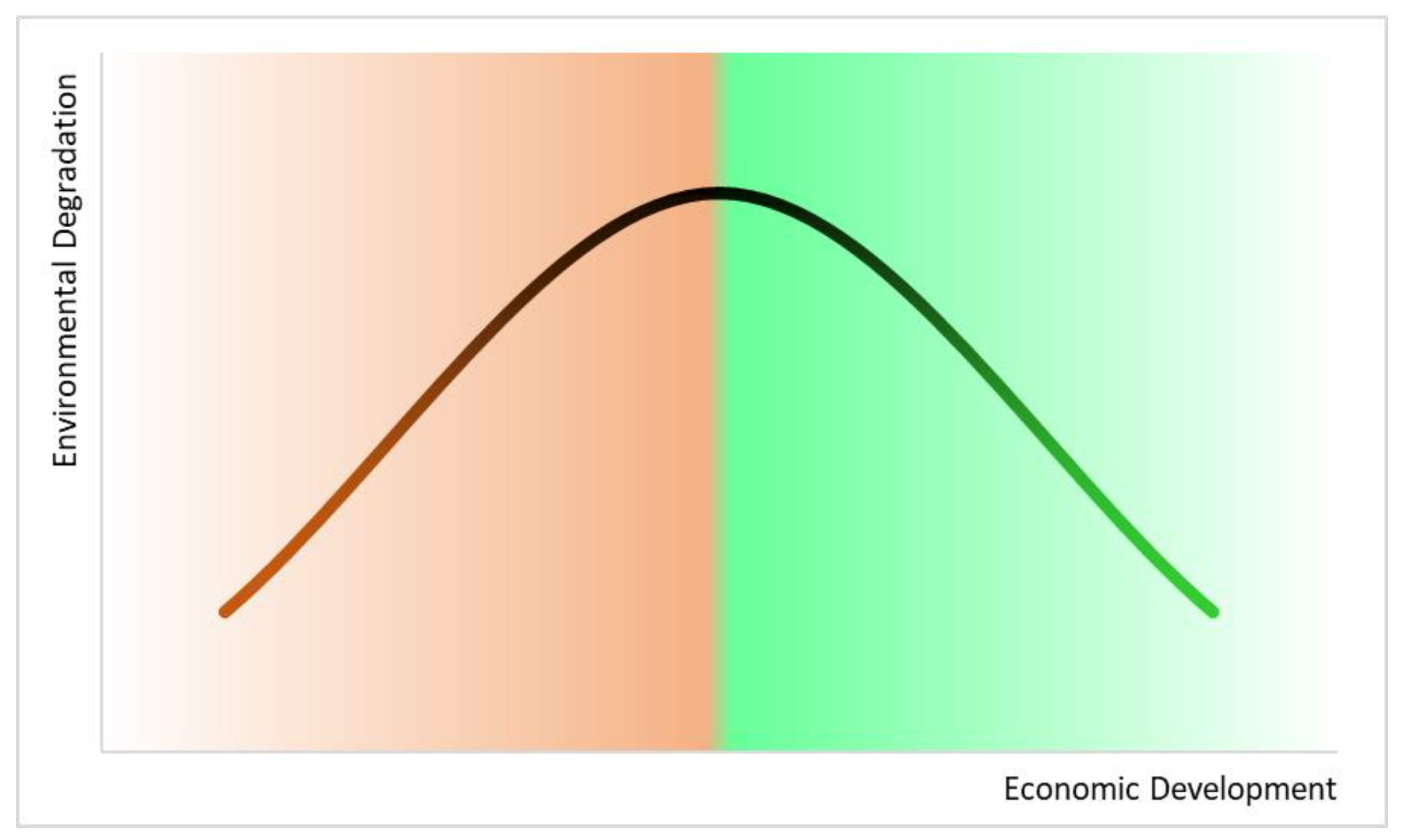
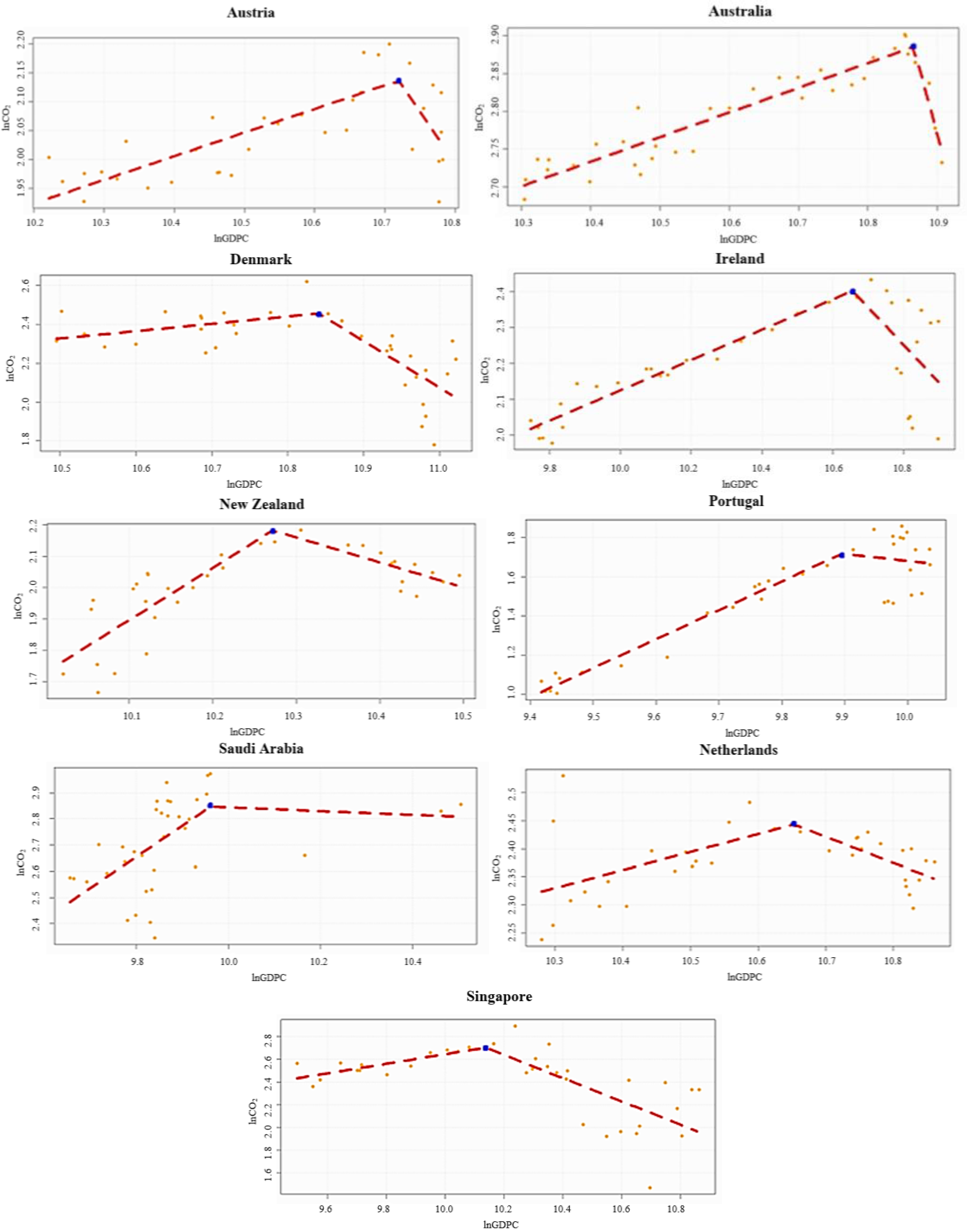
Then, the time-series kink regression model (Equation (4)) was run to capture the nonlinear relationship between economic growth and environmental quality as well as its turning point for each of the 17 countries where the kink effects had been detected. The results reveal that the EKC hypothesis holds in only nine countries, as graphically displayed in Figure 2. The nine countries found to have a statistically significant turning point of their economic growth and environmental quality relationship are Australia, Austria, the Netherlands, New Zealand, Portugal, Denmark, Ireland, Saudi Arabia, and Singapore. As is evident in Figure 2, in these countries, the early stages of economic growth were coupled with the rising CO₂ emissions up to the kink point; then, economic development beyond the kink point proceeded hand in hand with the declining CO₂ emissions. This empirical finding supports the EKC theory, which posits that the process of economic development is expected to do away with the environmental degradation created in the early stages of economic growth. This is probably because people in developed societies have the knowledge and a sense of environmental concern, and they push for the development and the use of green and clean technologies to improve environmental quality. Therefore, the time-series kink regression line will have a positive slope (${\beta }_1^{-}>0$) for the early stages of economic growth and a negative slope (${\beta }_1^{+}\le 0$) for the period beyond the kink point.

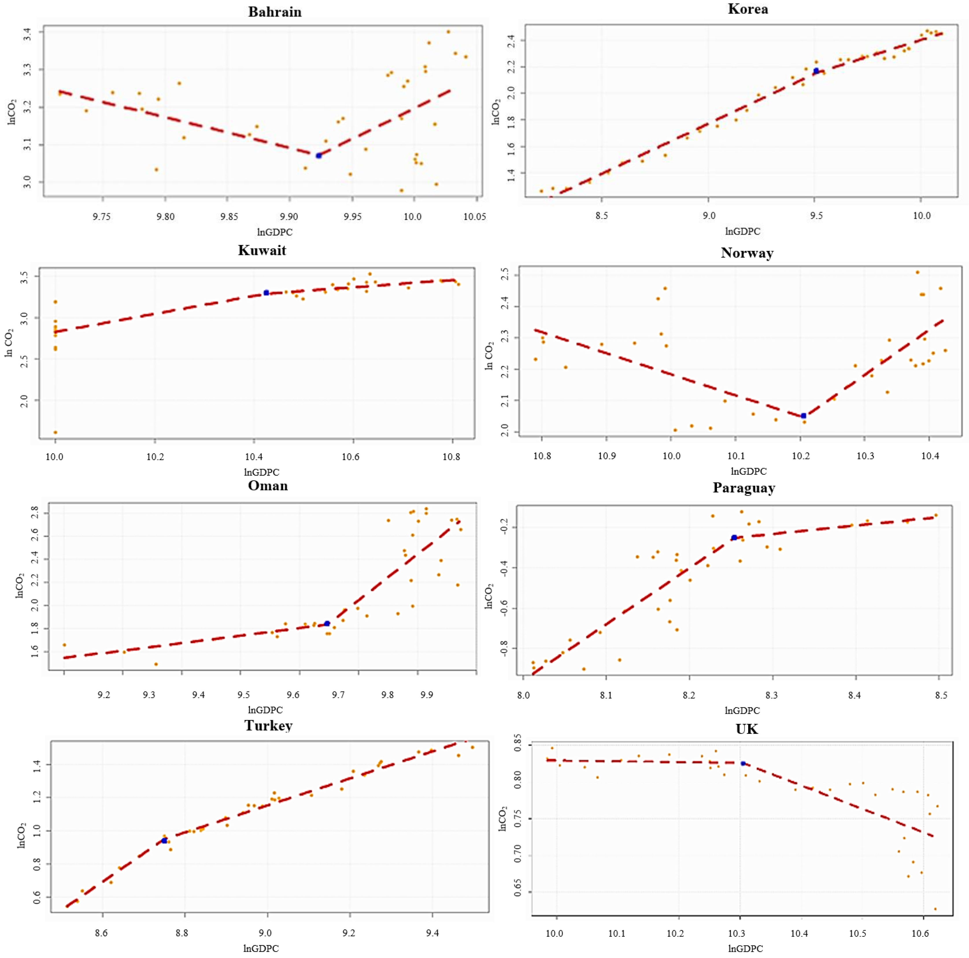
On the contrary, although Bahrain and Norway were found to have a lower CO₂ emissions trend along the economic growth process, the CO₂ emissions increased once their economies grew beyond the kink point. Some countries like Oman continued to have more critical environmental degradation with further economic growth. Meanwhile, in several countries, including Kuwait, Paraguay, South Korea, and Turkey, the level of CO₂ emissions still increased, but at a declining rate with economic development. Moreover, it is interesting to note that the UK is a country that could keep the level of CO₂ emissions constant along the path of economic growth and reduced the CO₂ emissions substantially after the country grew beyond the kink point. These evidences are illustrated in Figure 3.

After testing for the existence of a turning point and the nonlinear relationship between CO₂ emissions and GDPC, the next important issue necessitating the investigation is to find the level of economic growth that drives each of the nine countries with the EKC to lower environmental degradation. To this end, we have to locate the turning point of each country, which is estimated as $\gamma$ from the time-series kink regression model (Equation (4)), and convert it into the exponential form to provide the real GDP per capita (USD) level. Thus, the turning point corresponds to the economic growth level that needs to be kept to ensure the declining levels of environmental degradation. The estimated kink point and the corresponding real GDP per capita level for each of the nine countries with the EKC are presented in

Table 9. Estimated kink point and the corresponding real GDP per capita (USD) for countries empirically supporting the EKC hypothesis.

Country	$\mathbf{Kink} \mathbf{Point} (\mathit{\gamma })$	Real GDP Per Capita (USD)
Australia	10.871	52,627.81
Denmark	10.842	51,124.52
Austria	10.722	45,342.50
Ireland	10.669	43,001.92
Netherland	10.653	42,319.36
New Zealand	10.272	28,911.65
Singapore	10.140	25,336.47
Saudi Arabia	9.964	21,247.62
Portugal	9.901	19,950.31

Note: Real GDP per capita (USD) was obtained by converting the kink point value into the exponential form.

.

Table 9 shows the real GDP per capita that each country needs to maintain to ensure environmental sustainability; for example, the level for Australia is 52,359 USD, and that for Portugal is 19,843 USD.

The findings reported above enable us to know where the turning point of the relationship between economic growth and environmental degradation is. For the EKC hypothesis to hold, each country’s graph will have a positive slope at the early stages of economic growth and a negative slope when its economy grows past the turning point. The turning point of each country is determined from the estimation using the time-series kink regression model. Based on the value of the turning point coefficient, the corresponding real GDP per capita level can be identified, and it should be maintained or increased to support environmental sustainability.

6. Conclusions, Discussion, and Recommendations

6.1. Conclusions

This study examines the relationship between economic growth and environmental degradation measured by CO₂ emissions over the 1980−2016 period for 44 individual countries and the relationships between real GDP per capita, financial development, industrial sector, urbanization, and CO₂ emissions over the 2001–2016 period for eight groups of countries, including ASEAN, EFTA, EU, G7, GCC, Mercosur, NAFTA, and OECD using the time-series kink regression model and the panel kink regression model, respectively. Only 9 out of the 44 individual countries were found to have a relationship between growth and the environment in favor of the EKC hypothesis, as their income per capita once reached and increased beyond the kink point, it brought about declining CO₂ emissions. These countries are Australia, Austria, Netherlands, New Zealand, Portugal, Denmark, Ireland, Saudi Arabia, and Singapore. The results of the second model, the panel kink regression, indicated the EKC’s existence in the EU, OECD, and G7 because their economic development processes enabled the reduction and/or correction of the environmental degradation created in the early stages of their economic growth.

We found that both the time-series and panel analyses led to a mixed output. We observed that three out of the eight economic groups and 9 out of the 44 individual countries were found to have a growth and environment relationship in favor of the EKC hypothesis. Our study corresponds to the controversy of the existence of EKC in the literature. Although some groups and countries considered in this study confirm the EKC hypothesis (depicted by EKC curve; ${\beta }_1^{-}$ and ${\beta }_1^{+}$), a considerable number of economic groups and countries disconfirm the EKC relationship. If we consider the kink test results, we can observe a kink effect in 17 out of the 44 countries and all economic groups, but the inverted U-shaped relation of the EKC hypothesis is held in 9 out of the 44 countries and three out of the eight groups. Furthermore, we also explored a U-shaped relation in two countries (Bahrain and Norway), meaning that air pollution in terms of carbon dioxide emissions is influenced positively by economic growth when the real GDP per capita level exceeds its kink point. Moreover, we can explore a positive magnitude of the economic impact on CO₂ emissions in five individual countries (Korea, Kuwait, Paraguay, Oman, and Turkey) and two groups (GCC and Mercosur) when the real GDP per capita level exceeds its kink point. These results imply that the development of the economy undermines the environment by generating more pollution. Hence, it can be safely said that the sustained economic development in these countries and groups is not being pursued for clean energy production, and economic growth would not automatically clean the environment.

In addition, this study identifies the optimal levels of real GDP per capita that can support environmental sustainability for the individual countries and the groups of countries where the EKC hypothesis is empirically found to hold. This is done by the transformation of the kink point value into the real GDP per capita. Thus, for example, Australia should keep its real GDP per capita above 52,627.81 USD, and the EU should do so above 35,066.45 USD (for more details, see Table 6 for groups of countries and Table 9 for individual countries).

Furthermore, interesting results were obtained from the inclusion of four other control variables in the estimation model for groups of countries to explain the environmental quality. Financial development, industrialization, urbanization, and renewable energy consumption were found to increase CO₂ emissions, while renewable energy consumption appears to reduce environmental degradation. For financial development, the highest positive impact was shown in G7 with a value of 0.323. For industrialization, the highest positive impact was shown in Mercosur with a value of 0.532. For urbanization, the highest positive impact was shown in ASEAN with a value of 0.823. Finally, renewable energy consumption showed the highest negative impact in the EU with a value of −0.033. These results illustrate that the development of renewable energy consumption has an important role in the improvement of the environment.

Like other EKC literature, this study has some limitations based on which it offers suggestions for future research. In the first place, data availability constraints prevented us from carrying out the study with other possible factors affecting CO₂ emissions, such as solar radiation, air temperatures, trade openness, human capital, and total biocapacity. Second, this study does not fully describe what the indicator of environmental degradation used in the paper is. We considered only territorial CO₂ emission (production-based CO₂ emissions), which means that the impact of commercial trade and the externalization of polluting activities from high-environmental-burden products are not considered. Thus, the CO₂ emission footprint (consumption-based approach) is suggested for future studies. The CO₂ emission footprint is well discussed in Quéré et al. [49] and Fanning and O’Neill [50]. Finally, future studies can explore the EKC’s existence using other econometric models, such as the generalized method of moments and the panel smooth kink regression approach.

6.2. Policy Implications

In most countries and groups of countries under investigation, this study found that economic growth could not always lead to the improvement of environmental quality. Consequently, policymakers must strategically devise and implement some interventions to promote economic growth side by side with the environmental quality improvement for sustainable development. Considering the finding that financial development might facilitate investment in economic activities that produce environmental pollution as a by-product, financial institutions or authorizes should give priority to credit provision for investment in the use and development of clean and green technology, perhaps by charging a lower interest rate on agreements about environmental protection or the implementation of carbon footprints. For countries with prominent industrial sectors that contributed to the elevated CO₂ emissions, policies should be enacted to promote more activities in tertiary industry, like service and finance, or to encourage the secondary industry to adopt clean and environmentally friendly technology. This is to say, green finance is an environmentally friendly solution for achieving economic and environmental sustainability. Furthermore, as industrialization and urbanization contribute to a negative impact on the environment, a strict carbon tax policy, monetary policy, and migration policy could assist in reducing the environmental risk. Industrialization and urbanization raise environmental degradation in many economic groups; therefore, green business incentives and green public transportation are required. Finally, it was found that the promotion of renewable energy brings environmental benefits. Therefore, research and development of technologies are essential for the generation of renewable energy sources and related infrastructure.

References

- Intergovernmental Panel on Climate Change. Global Warming of 1.5 °C. 2018. Available online: https://www.ipcc.ch/site/assets/uploads/sites/2/2018/07/SR15_SPM_High_Res.pdf (accessed on 24 December 2018).
- Grossman, G.M.; Krueger, A.B. Environmental Impacts of a North American Free Trade Agreement; National Bureau of Economic Research; MIT Press: Cambridge, MA, USA, 1991. [Google Scholar]
- Kuznets, S. Economic Growth and Income Inequality. Am. Econ. Rev. 2019, 45, 25–37. [Google Scholar] [CrossRef]
- Al-Mulali, U.; Tang, C.F.; Ozturk, I. Estimating the Environment Kuznets Curve hypothesis: Evidence from Latin America and the Caribbean countries. Renew. Sustain. Energy Rev. 2015, 50, 918–924. [Google Scholar] [CrossRef]
- Hanif, I.; Gago-De-Santos, P. The importance of population control and macroeconomic stability to reducing environmental degradation: An empirical test of the environmental Kuznets curve for developing countries. Environ. Dev. 2017, 23, 1–9. [Google Scholar] [CrossRef]
- Ulucak, R.; Bilgili, F. A reinvestigation of EKC model by ecological footprint measurement for high, middle and low income countries. J. Clean. Prod. 2018, 188, 144–157. [Google Scholar] [CrossRef]
- Akbostancı, E.; Türüt-Aşık, S.; Tunç, G.I. The relationship between income and environment in Turkey: Is there an environmental Kuznets curve. Energy Policy 2009, 37, 861–867. [Google Scholar] [CrossRef]
- Özokcu, S.; Özdemir, Ö. Economic growth, energy, and environmental Kuznets curve. Renew. Sustain. Energy Rev. 2017, 72, 639–647. [Google Scholar] [CrossRef]
- Das Neves Almeida, T.A.; Cruz, L.; Barata, E.; García-Sánchez, I.-M. Economic growth and environmental impacts: An analysis based on a composite index of environmental damage. Ecol. Indic. 2017, 76, 119–130. [Google Scholar] [CrossRef]
- Intergovernmental Panel on Climate Change. Climate Change 2014 Synthesis Report. 2014. Available online: https://www.ipcc.ch/site/assets/uploads/2018/02/SYR_AR5_FINAL_full.pdf (accessed on 24 December 2018).
- Atasoy, B.S. Testing the environmental Kuznets curve hypothesis across the U.S.: Evidence from panel mean group estimators. Renew. Sustain. Energy Rev. 2017, 77, 731–747. [Google Scholar] [CrossRef]
- Sinha, A.; Shahbaz, M. Estimation of Environmental Kuznets Curve for CO2 emission: Role of renewable energy generation in India. Renew. Energy 2018, 119, 703–711. [Google Scholar] [CrossRef] [Green Version]
- Shahbaz, M.; Tiwari, A.K.; Nasir, M. The effects of financial development, economic growth, coal consumption and trade openness on CO2 emissions in South Africa. Energy Policy 2013, 61, 1452–1459. [Google Scholar] [CrossRef] [Green Version]
- Pata, U.K. Renewable energy consumption, urbanization, financial development, income and CO2 emissions in Turkey: Testing EKC hypothesis with structural breaks. J. Clean. Prod. 2018, 187, 770–779. [Google Scholar] [CrossRef]
- Liu, X.; Bae, J. Urbanization and industrialization impact of CO2 emissions in China. J. Clean. Prod. 2018, 172, 178–186. [Google Scholar] [CrossRef]
- Shahbaz, M.; Solarin, S.A.; Ozturk, I. Environmental Kuznets Curve hypothesis and the role of globalization in selected African countries. Ecol. Indic. 2016, 67, 623–636. [Google Scholar] [CrossRef] [Green Version]
- Bekhet, H.A.; Othman, N.S. The role of renewable energy to validate dynamic interaction between CO2 emissions and GDP toward sustainable development in Malaysia. Energy Econ. 2018, 72, 47–61. [Google Scholar] [CrossRef]
- Aruga, K. Investigating the Energy-Environmental Kuznets Curve Hypothesis for the Asia-Pacific Region. Sustainability 2019, 11, 2395. [Google Scholar] [CrossRef] [Green Version]
- Ahmad, N.; Du, L.; Lu, J.; Wang, J.; Li, H.-Z.; Hashmi, M.Z. Modelling the CO2 emissions and economic growth in Croatia: Is there any environmental Kuznets curve. Energy 2017, 123, 164–172. [Google Scholar] [CrossRef]
- Stern, D.I. The Rise and Fall of the Environmental Kuznets Curve. World Dev. 2004, 32, 1419–1439. [Google Scholar] [CrossRef]
- Kaika, D.; Zervas, E. The Environmental Kuznets Curve (EKC) theory—Part A: Concept, causes and the CO2 emissions case. Energy Policy 2013, 62, 1392–1402. [Google Scholar] [CrossRef]
- Pata, U.K. The influence of coal and noncarbohydrate energy consumption on CO2 emissions: Revisiting the environmental Kuznets curve hypothesis for Turkey. Energy 2018, 160, 1115–1123. [Google Scholar] [CrossRef]
- Koilo, V. Evidence of the Environmental Kuznets Curve: Unleashing the Opportunity of Industry 4.0 in Emerging Economies. J. Risk Financ. Manag. 2019, 12, 122. [Google Scholar] [CrossRef] [Green Version]
- Pal, D.; Mitra, S.K. The environmental Kuznets curve for carbon dioxide in India and China: Growth and pollution at crossroad. J. Policy Model. 2017, 39, 371–385. [Google Scholar] [CrossRef]
- Mikayilov, J.I.; Galeotti, M.; Hasanov, F.J. The Impact of Economic Growth on CO2 Emissions in Azerbaijan; No. 102; IEFE, Center for Research on Energy and Environmental Economics and Policy, Universita’Bocconi: Milano, Italy, 2018. [Google Scholar]
- Moutinho, V.; Varum, C.; Madaleno, M. How economic growth affects emissions? An investigation of the environmental Kuznets curve in Portuguese and Spanish economic activity sectors. Energy Policy 2017, 106, 326–344. [Google Scholar] [CrossRef]
- Shahbaz, M.; Solarin, S.A.; Mahmood, H.; Arouri, M.E.H. Does financial development reduce CO2 emissions in Malaysian economy? A time series analysis. Econ. Model. 2013, 35, 145–152. [Google Scholar] [CrossRef] [Green Version]
- Boutabba, M.A. The impact of financial development, income, energy and trade on carbon emissions: Evidence from the Indian economy. Econ. Model. 2014, 40, 33–41. [Google Scholar] [CrossRef] [Green Version]
- Bilgili, F.; Koçak, E.; Bulut, Ü. The dynamic impact of renewable energy consumption on CO2 emissions: A revisited Environmental Kuznets Curve approach. Renew. Sustain. Energy Rev. 2016, 54, 838–845. [Google Scholar] [CrossRef]
- Saidi, K.; Omri, A. The impact of renewable energy on carbon emissions and economic growth in 15 major renewable energy-consuming countries. Environ. Res. 2020, 186, 109567. [Google Scholar] [CrossRef]
- Bhattacharya, M.; Churchill, S.A.; Paramati, S.R. The dynamic impact of renewable energy and institutions on economic output and CO2 emissions across regions. Renew. Energy 2017, 111, 157–167. [Google Scholar] [CrossRef]
- Ali, R.; Bakhsh, K.; Yasin, M.A. Impact of urbanization on CO2 emissions in emerging economy: Evidence from Pakistan. Sustain. Cities Soc. 2019, 48, 101553. [Google Scholar] [CrossRef]
- Zafar, A.; Ullah, S.; Majeed, M.T.; Yasmeen, R. Environmental pollution in Asian economies: Does the industrialisation matter? OPEC Energy Rev. 2020, 44, 227–248. [Google Scholar] [CrossRef]
- Maneejuk, P.; Yamaka, W.; Sriboonchitta, S. Does the Kuznets curve exist in Thailand? A two decades’ perspective (1993–2015). Ann. Oper. Res. 2019, 1–32. [Google Scholar] [CrossRef]
- Hansen, B.E. Regression Kink with an Unknown Threshold. J. Bus. Econ. Stat. 2017, 35, 228–240. [Google Scholar] [CrossRef]
- Zhang, Y.; Zhou, Q.; Jiang, L. Panel kink regression with an unknown threshold. Econ. Lett. 2017, 157, 116–121. [Google Scholar] [CrossRef]
- Lee, S.-Y.; Song, X.-Y. Evaluation of the Bayesian and Maximum Likelihood Approaches in Analyzing Structural Equation Models with Small Sample Sizes. Multivar. Behav. Res. 2004, 39, 653–686. [Google Scholar] [CrossRef]
- Van De Schoot, R.; Broere, J.J.; Perryck, K.H.; Zondervan-Zwijnenburg, M.; Van Loey, N.E. Analyzing small data sets using Bayesian estimation: The case of posttraumatic stress symptoms following mechanical ventilation in burn survivors. Eur. J. Psychotraumatol. 2015, 6, 25216. [Google Scholar] [CrossRef]
- Muthén, L.K.; Muthén, B.O. How to use a Monte Carlo study to decide on sample size and determine power. Struct. Equ. Model. 2002, 9, 599–620. [Google Scholar] [CrossRef]
- Tarkhamtham, P.; Yamaka, W. High-Order Generalized Maximum Entropy Estimator in Kink Regression Model. Thai J. Math. 2019, 185–200. Available online: http://thaijmath.in.cmu.ac.th/index.php/thaijmath/article/view/3914 (accessed on 1 November 2020).
- Levin, A.; Lin, C.-F.; Chu, C.-S.J. Unit root tests in panel data: Asymptotic and finite-sample properties. J. Econom. 2002, 108, 1–24. [Google Scholar] [CrossRef]
- Dickey, D.A.; Fuller, W.A. Distribution of the estimators for autoregressive time series with a unit root. J. Am. Stat. Assoc. 1979, 74, 427–431. [Google Scholar]
- Shahbaz, M.; Shahzad, S.J.H.; Ahmad, N.; Alam, S. Financial development and environmental quality: The way forward. Energy Policy 2016, 98, 353–364. [Google Scholar] [CrossRef] [Green Version]
- Shahbaz, M.; Shahzad, S.J.H.; Alam, S.; Apergis, N. Globalisation, economic growth and energy consumption in the BRICS region: The importance of asymmetries. J. Int. Trade Econ. Dev. 2018, 27, 985–1009. [Google Scholar] [CrossRef] [Green Version]
- Kiliç, C.; Balan, F. Is there an environmental Kuznets inverted-U shaped curve? Panoeconomicus 2018, 65, 79–94. [Google Scholar] [CrossRef] [Green Version]
- Shoaib, H.M.; Rafique, M.Z.; Nadeem, A.M.; Huang, S. Impact of financial development on CO2 emissions: A comparative analysis of developing countries (D8) and developed countries (G8). Environ. Sci. Pollut. Res. Int. 2020, 27, 12461–12475. [Google Scholar] [CrossRef]
- Halliru, A.M.; Loganathan, N.; Hassan, A.A.G.; Mardani, A.; Kamyab, H. Re-examining the environmental Kuznets curve hypothesis in the Economic Community of West African States: A panel quantile regression approach. J. Clean. Prod. 2020, 276, 124247. [Google Scholar] [CrossRef]
- Engle, R.F.; Yoo, B.S. Forecasting and testing in co-integrated systems. J. Econom. 1987, 35, 143–159. [Google Scholar] [CrossRef]
- Le Quéré, C.; Andrew, R.M.; Friedlingstein, P.; Sitch, S.; Pongratz, J.; Manning, A.C.; Korsbakken, J.I.; Peters, G.P.; Canadell, J.G.; Jackson, R.B.; et al. Global Carbon Budget 2017. Earth Syst. Sci. Data 2018, 10, 405–448. [Google Scholar] [CrossRef] [Green Version]
- Fanning, A.L.; O’Neill, D.W. The Wellbeing–Consumption paradox: Happiness, health, income, and carbon emissions in growing versus non-growing economies. J. Clean. Prod. 2019, 212, 810–821. [Google Scholar] [CrossRef]
Figure 1.
Environmental Kuznets Curve.
Figure 2.
Empirical findings on the relationship between lnCO2 emissions and lnGDPC for individual countries supporting the Environmental Kuznets Curve (EKC) hypothesis.
Figure 3.
Empirical findings on the relationship between lnCO2 emissions and lnGDPC for individual countries not supporting the Environmental Kuznets Curve (EKC) hypothesis.