Closed-Loop Supply Chain Coordination under a Reward–Penalty and a Manufacturer’s Subsidy Policy


1
Port Investment and Operation Department, Korea Maritime Institute, Busan 49111, Korea
2
College of Business Administration, Sejong University, Seoul 05006, Korea
3
College of Business Administration, Seoul National University, Seoul 08826, Korea
*
Author to whom correspondence should be addressed.
Sustainability 2020, 12(22), 9329; https://0-doi-org.brum.beds.ac.uk/10.3390/su12229329
Submission received: 14 October 2020
/
Revised: 4 November 2020
/
Accepted: 5 November 2020
/
Published: 10 November 2020
(This article belongs to the Section Economic and Business Aspects of Sustainability)
Abstract
:Government legislation significantly impacts closed-loop supply chain (CLSC) operations. This study examines the collection rate of and decisions on the product greening improvement level in a three-level CLSC with the government’s reward–penalty and a manufacturer’s subsidy policy. Four game-theoretic models are analyzed in order to evaluate the ways in which the policy and revenue-sharing contracts (RSCs) between the manufacturer and retailer affect the CLSC members’ optimal decisions and profits. We found that a reward–penalty and subsidy policy raise the collection rate, as well as the product greening improvement level. A manufacturer’s financial conflict of interest can be mitigated using RSCs. The RSCs between the manufacturer and the retailer also increase the profit of a recycling company that successfully coordinates the CLSC. An interesting result is that, when the RSCs are used under the subsidy policy, the collection rate is higher than it is in a centralized model. We also found that the subsidy level needs to be adjusted according to the price of the recycling resources, and that increasing the value of the recyclable resources and lowering the recycling costs in the early stages of the supply chain collaboration could lead to higher environmental sustainability. These results illustrate that using an RSC can effectively coordinate the CLSC, and can thus help policy implementation by governments.
1. Introduction
A closed-loop supply chain (CLSC) is the combination of a forward and a reverse supply chain. Industrial and academic circles are paying attention to CLSCs in both their economic and environmental aspects. A CLSC has the great potential to be economically feasible [1]. A typical example is urban mines extracting and using rare metals from waste electronic equipment and cars. Moreover, the CLSC reduces the environmental pollution caused by harmful substances. Governments encourage the CLSCs to mitigate environmental problems. Governments strive to promote the circulation of resources through recycling, and to reduce environmental pollution by applying regulations. For example, the EU controls the use of harmful substances in electronic equipment through its 2003 Waste Electrical and Electronic Equipment (WEEE) directive. Denmark developed the Extended Producer Responsibility (EPR) system in 1990 to encourage manufacturers to make environment-friendly products and to take responsibility for recycling costs. EPR is a policy approach that gives the financial or physical responsibility for the treatment of consumed products to manufacturers. The detailed methods vary slightly from country to country; this system has now been implemented by many OECD (Organization for Economic Cooperation and Development) countries [2].
Korea also operates the EPR system, in order to keep pace with the global trend. Korea’s EPR system requires manufacturers to recycle a certain amount of waste every year, such as products or packaging materials such as batteries, tires, lubricants, and synthetic resins. In addition, the government imposes penalties if the recycling rate does not meet the regulation level. Most manufacturers do their duty by subsidizing recycling companies instead of directly recycling under the government’s acceptance. Many countries use a similar policy, but thus far, few studies have examined the ways in which government legislation (the reward–penalty system) and manufacturer’s subsidies affect the decisions of CLSC members.
In order to bridge this gap in the literature, this study uses game theory to compare the optimal collection rate and product greening improvement level of a CLSC with and without government legislation. In this context, the collection rate represents the proportion of the products collected for recycling. Since policies such as the 2003 WEEE directive and EPR primarily aim to raise the collection rate, it has gained attention as a key variable in CLSC research. Similarly, the product greening improvement level, which has a significant influence on the production costs and market demand, measures the degree of a product’s environmental friendliness [3]. Restrictions on using harmful substances or product designs that consider recycling, as prescribed by the Eco-Assurance System of Electrical and Electronic Equipment and Vehicles, are some examples of product greening improvements in Korea. Furthermore, this study also examines whether supply chain coordination through contracts, especially Revenue-Sharing Contracts (RSCs) between the manufacturer and the retailer, improves the performance in CLSCs under government legislation. RSC is one of most popular supply chain coordination contracts, in which a manufacturer provides products to a retailer at prices lower than the wholesale price, while a retailer shares a certain ratio of its revenue with the manufacturer [4]. In particular, we aim to answer the following research questions:
- Can a reward–penalty system and manufacturer subsidies increase the collection rate and product greening improvement level?
- Is it possible to raise the collection rate, product greening improvement level, and members’ profits by implementing RSCs, even in CLSCs under government legislation?
- How do changes in the parameters related to recycling resources affect decision-making and performance?
We find that the reward–penalty system and manufacturer’s subsidies increase both the collection rate and the product greening improvement level in three-level CLSCs, and that perfect coordination for collection rates can be achieved, depending on the intensity of the reward–penalty. However, an intense penalty decreases manufacturers’ profits. We show that the profits of all of the supply chain members can be increased by implementing RSCs between the manufacturer and the retailer, and that collection rates greater than those in a centralized model can also be achieved. Moreover, we suggest that adjusting subsidies based on the price change of recyclable resources is necessary by numerical analysis. Increasing the value of recyclable resources and lowering recycling costs is also important for environmental sustainability. The novelty of this paper is that it proposes a CLSC coordination in terms of profit and collection rates using RSC, and suggests future policy directions for environmental sustainability. This result provides many managerial implications for decision-making by CLSC members.
The remainder of this paper is structured as follows. Section 2 provides a literature review, and Section 3 presents the game theory analysis. Section 4 provides a comparative analysis of each model’s results, and Section 5 provides a numerical analysis. Section 6 presents the managerial implications. Lastly, Section 7 summarizes the results and presents topics for future research.
2. Literature Review
Theoretical studies using game theory follow two research trends: (1) CLSC performance according to the channel leadership, collection agent, and coordination through contracts; and (2) the roles and effects of government intervention.
2.1. CLSC Performance According to the Channel Leadership, Collection Agent, and Coordination
Studies of CLSCs using game theory have mostly examined the ways in which their performance varies depending on the channel leadership and collection agent. Maiti and Giri [5], Zerang et al. [6], and Jafari et al. [7] compared the performance of various supply chain models according to channel leadership, and identified the conditions needed to achieve the best performance. Huang et al. [8], Huang and Wang [9], Liu et al. [10], and Modak et al. [11] compared the performance of supply chains under various collection channel structures. Their results showed that the collection channel structure affects the supply chain performance and the collection rate. In summary, while these studies analyzed the performance of CLSCs in various situations, they did not examine whether the coordination methods improve performance.
Several researchers have investigated coordination strategies, considering waste recycling collection and management. Savaskan et al. [12] compared the performance of a supply chain by dividing it into the cases in which the manufacturer directly collects, the retailer collects, and the collector collects the waste materials. They claimed that two-part tariff contracts improve performance. De Giovanni [13] compared the performance of wholesale price contracts and RSCs in a CLSC comprising a manufacturer and a retailer. Choi et al. [14] analyzed the performance in a three-level supply chain. They claimed that two-part tariff contracts and RSCs optimize the performance. Han et al. [15] compared the performance in the cases in which the manufacturer or the retailer collects waste materials when there is a disruption in the reprocessing cost. They argued that RSCs could better handle cost disruption. Zheng et al. [16] compared supply chain performance according to the power structure in dual-channel CLSCs. They claimed that two-part tariff contracts perform better than wholesale price contracts. Taleizadeh et al. [17] claimed that a manufacturer performs better in a dual-channel forward/dual-channel reverse supply chain than in a single-channel forward/dual-channel reverse supply chain. They also showed that the supply chain performance might improve using a contract combining collaborative advertising and two-part tariffs. In summary, the above studies studied the type of contract that raises supply chain performance; However, they have not examined the effects of a government’s policy.
2.2. The Roles and Effects of Government Intervention
Although the literature on supply chain coordination is broad, few studies have considered the effect of government policies. Wang et al. [18] studied the ways in which the government’s reward–penalty system in a two-level supply chain affects performance, and showed that the system increases the collection rate, and that applying a higher reward–penalty to the collector raises the performance of the collector-dominated model. Wang et al. [19] compared the ways in which the government’s reward–penalty system affects performance when one manufacturer acts as the leader in a supply chain consisting of two manufacturers and one retailer. They showed that the collection rate increases under a reward–penalty system, as do the profits of the dominating manufacturer and retailer. Wang et al. [20] studied whether the government’s reward–penalty system can promote the retailer’s collection when the manufacturer is not aware of the retailer’s collection efforts. They found that the reward–penalty system might help increase the collection rate by increasing the waste material price. This study differs from the abovementioned studies, as it assumes a two-level supply chain and focuses on whether the reward–penalty system has different effects on dominating and following manufacturers. Moreover, they do not consider the manufacturer’s subsidy.
2.3. Contribution to the Literature
While the aforementioned studies make a significant contribution to the body of knowledge on environmental sustainability, few provide guidelines for government legislation and subsidy-setting in this area. Except for Wang et al. [18,19,20], who examined the impact of the government’s role, the researchers have generally sought to identify which party among the manufacturer, retailer, and third party (e.g., collector) takes the leading role. However, given the government’s importance in the waste collection decision-making process, and its significant role in maximizing CLSC profit, this study investigates the influence of the reward–penalty mechanism (RPM) with a subsidy policy on economic and environmental performance (i.e., the collection rate and performance greening improvement level) of supply chains. This approach is novel in that it enables us to compare the supply chain’s performance with that under the existing system by including the reward–penalty system and the manufacturer subsidy into the model, as prescribed by the EPR system.
Second, instead of focusing on the channel leadership, this study establishes models of a three-level supply chain with a manufacturer, a retailer, and a recycling company, and investigates the coordination approach using an RSC in order to appropriately demonstrate a real-world case in Korea. Because RSCs have become an essential tool in corporate governance, such as partnership management through profit and cost sharing [21], this study proposes and evaluates the effectiveness of RSCs for the improvement of environmental and economic performance.
Finally, the main contribution of this work is the suggestion of a strategic subsidy policy based on recyclable resource prices. In particular, the examination of the influence of government legislation and supply chain contracts in CLSCs on environmental performance differentiates this study from others. Hence, it bridges the gap between CLSC models and governments’ legislation for three-level supply chain coordination by applying a game theoretic approach. Table 1 summarizes the body of knowledge on this topic.
3. Research Model and Analysis
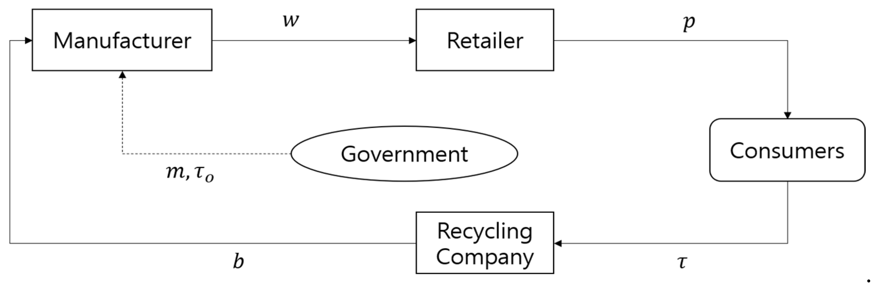
This study sets a CLSC comprising one manufacturer, one retailer, and one recycling company, and analyzes a manufacturer Stackelberg game. The supply chain literature commonly assumes that the manufacturer is set as a Stackleberg leader [4,5,35] and that EPR is a manufacturer-centered policy approach. Figure 1 shows the CLSC structure considered in this study, and Table 2 describes the key notations.
The supply chain adopts a wholesale price contract. Equations (1)–(3) show the profit functions:
The manufacturer determines the wholesale price and the product greening improvement level. The retailer sets the retail price. The recycling company determines the collection ratio of the used product (waste material) and processes it to extract raw materials or turns it into a recyclable resource, and then sells it to the manufacturer.
Assumption 1.
Product demand is the function of the price and product greening improvement level.
The product greening improvement level increases the satisfaction of consumers, thus increasing demand [3]. Many studies in operations management use such linear demand functions [36]. In most cases, the product greening improvement level does not have a greater effect than the price, and thus, we assume that is between 0 and 1 [35].
Assumption 2.
The cost required to increase the product greening improvement level is in the form of a quadratic function. Moreover, the coefficient of the cost is assumed to follow El Ouardighi’s [4] assumption of a constant coefficient.
Assumption 3.
The product’s manufacturing cost is presumed to increase along with the product’s greening improvement level, which is presented asin order to depict the tradeoff. The product’s greening improvement level increases the manufacturing cost, as the replacement of harmful substances or changing product structures incurs additional costs. However, in order to avoid the situation in which the incentive for the manufacturer to invest in quality no longer exists, we assume that the product greening improvement level has a greater effect on demand than it does on the manufacturing cost.
Assumption 4.
We assume that the value of the recyclable resources is above its price. represents the net worth produced when the manufacturer uses recyclable resources. Here, the net worth is represented by the economic value—such as a cost reduction [11]—or the intangible value, such as an improvement in social reputation [19].
Assumption 5.
Assumption 6.
The prices of the recyclable resources are exogenous variables. These prices are mostly affected by the prices of the raw materials. For example, recycled polypropylene is affected by international oil prices. Maiti and Giri [5] used the same assumption, that the recycling price of used products is an exogenous variable. Moreover, we assume that such prices are always above the processing costs
Assumption 7.
The cost of the recycling company’s effort to increase the collection rate is represented in the form of a square, as is the case for the product greening improvement level, with the coefficient
Assumption 8.
When the cost of the recycling company’s effort () is greater than a certain value, we ensure that the collection rate does not exceed 1, thereby satisfying all of the the conditions presented in the analysis [6,10]. We describe, in the Appendix, the condition ofthat the collection rates are between 0 and 1, as a lemma.
We aim to provide the implications by comparing the optimal performance of the supply chain under four models: the centralized model (CM), the wholesale price model (WP), the wholesale price under government legislation model (WPG), and the revenue-sharing under government legislation model (RSG).
3.1. CM
In the CM, the supply chain’s profit function is
In Equation (5), we obtain the following results.
Proposition 1.
If (i), (ii)are satisfied, the optimal solutions of CM are as follows:
.
Proof.
See Appendix A. The condition of
is that the is between 0 and 1, as shown in Lemma 1 (Appendix B). □
3.2. WP
In the WP, each member maximizes their own profits. The manufacturer determines the wholesale price and product greening improvement level, while the retailer and the recycling company determine their own profits for each unit and collection rate. The following results can be obtained using backward induction.
Proposition 2.
The optimal solutions in the WP are presented as follows:
Proof.
See the Appendix A. The condition of is that the is between 0 and 1, as is shown in Lemma 2 (Appendix B). □
3.3. WPG
This model is the same as the WP, but with government legislation. Equations (17)–(19) show the profit functions:
The government sets as the mandatory collection rate, and it imposes a levy of for falling short, and a reward for exceeding the amount. The processes of collecting, selecting, and reprocessing the used products are different from those performed by the manufacturer. Since the establishment of such recycling processes requires significant time and costs, most manufacturers entrust recycling to specialist companies instead of fulfilling the duty themselves, as is permitted under the regulations. In the equation, is the coefficient representing the proportion of the expenses covered by the manufacturer, and it lies between 0 and s ).
The manufacturer first decides and presents it to the recycling company. Then, the wholesale price and product greening improvement level are decided, as they are in the WP. Finally, the retailer and recycling company decide the profit for each unit and the collection rate, respectively. The following results can be obtained using backward induction.
Proposition 3.
The optimal solutions in the WPG are presented as follows:
Proof.
See the Appendix A. The condition of is that the is between 0 and 1, as shown in Lemma 3 (Appendix B). □
The optimal value of appears to have a certain value deducted from the value of , indicating that the assumption is satisfied. For other values, the terms for are added, and appear in a more complex form than the WP. only affects the manufacturer’s optimal profit, and does not affect the other values, because the EPR only imposes responsibility on the manufacturers.
3.4. RSG
In an RSC, the manufacturer shares the retailer’s profits at a certain percentage. In order to generate more profits by eliminating double marginalization, the wholesale price in the RSC must be set lower than that in the wholesale price contract. For the wholesale price to be lower than the unit cost [37,38,39], we assume that both parties agree with ). Here, indicates the retailer’s share of the total profits. We also apply the optimum subsidy obtained in the previous section [Equation (21)]. This keeps the subsidy from being lower than 0. The profit functions of the members are as follows:
The manufacturer first presents to the retailer. We cannot obtain the optimum for the manufacturer. Here, we assume as a constant, after which we analyze the scope of that can show better performance than that under the WPG. The manufacturer decides the product greening improvement level with a fixed wholesale price; then, the retailer decides the price, and the recycling company decides the collection rate. Likewise, the following results can be obtained using backward induction.
Proposition 4.
The optimal solutions in the RSG are as follows:
is described in Appendix.
Proof.
See Appendix A. The condition of
is that the is between 0 and 1, as shown in Lemma 4 (Appendix B). □
Putting the above results into Equations (28)–(30) provides the equation for each member’s optimum profit, but the form is so complicated that it is not included here.
4. Results
This section compares the performance of each model using the optimal solutions presented in Section 3.
4.1. CM and WP
The following results can be obtained by comparing the performances of the CM and WP.
Proposition 5.
In the WP, the collection rate and product greening improvement level become lower than those in the CM:
Proof.
See the Appendix A. □
Proposition 6.
In the WP, the sum of all of the members’ profits becomes smaller than that in the CM:
Proof.
See the Appendix A. □
This result generally indicates that inefficiency due to double marginalization exists in CLSCs. This inefficiency lowers the economic performance, which adversely affects its environmental performance as well.
4.2. WP and WPG
The following results can be obtained by comparing the performance of the WPG and WP.
Proposition 7.
Under government legislation, the collection rate and product greening improvement level are higher than those in the WP:
Proof.
See the Appendix A. □
Proposition 8.
Under government legislation, the profits of the retailer and recycling company are higher than those in the WP, and the manufacturer’s profits vary depending on the mandatory recycling rates and penalty intensity:
are described in the Appendix.
Proof.
See the Appendix A. □
The profits of the retailer and recycling company increase compared with the WP. The manufacturer’s profits always decrease compared with the WP if the mandatory recycling rate is above a certain level and the intensity of the reward–penalty is within a certain interval. This may be because a lower mandatory recycling rate is easier to achieve, and thus, the manufacturer is more likely to receive a reward from the government. When the mandatory recycling rate is above a certain level, profits tend to be lower than those in the WP when the intensity of the reward–penalty is within a certain interval.
Special case.
Perfect coordination in terms of the collection rate.
Here, we analyze the reward–penalty intensity and manufacturer’s profit when the collection rate in the WPG becomes the same as the CM. In general, the studies of supply chain coordination refer to the case in which the performance of the decentralized model equals that of the CM as ‘perfect coordination’. Because the government implements policies to increase the collection rate, perfect coordination occurs when the collection rate in the CM is the same as that in the WPG.
Proposition 9.
Under the following reward–penalty intensity, the collection rates of the WPG and CM become the same. Here, if the collection rate is defined as the mandatory recycling rate, the manufacturer’s profit is always lower than that in the WP:
Proof.
See the Appendix A. □
The CM’s performance is used as the ideal value in many theoretical analyses. In other words, for the government to raise the collection rate to the ideal level, the reward–penalty intensity is set very high, and the manufacturer pays more to achieve this goal; hence, the profit decreases. In conclusion, if the government increases the policy intensity to achieve the goal under the current EPR, the environmental performance improves as intended, whereas the profit of the manufacturer is likely to decrease.
4.3. WPG and RSG
The following results can be obtained by comparing the performances of the WPG and RSG.
Proposition 10.
The collection rate in the RSG is always higher than that in the WPG, and there is the range ofin which the product greening improvement level becomes higher than that in the WPG:
Proof.
See the Appendix A. □
Even if the same subsidy is applied as in the WPG, the collection rate is higher in the RSG. The product greening improvement level becomes higher than that in the WPG if the manufacturer takes more than a certain proportion of the revenue.
Proposition 11.
The recycling company’s profit is always higher than that in the WPG, and there is the range ofin which the manufacturer’s profit becomes higher than that in the WPG:
Proof.
See the Appendix A. □
If an RSC is implemented, demand will increase, which enables the manufacturer and retailer to make higher profits. The collection of the used products will increase with the demand, and thus the profit of the recycling company will also increase. This increased profit will lead to an increase in the collection rate. That is, even if the recycling company is not directly involved in the contract, the general performance under the CLSC can improve. The manufacturer’s profits increase more than those in the WPG when its distribution ratio is above a certain level. This fact indicates that the problem in which the manufacturer’s profit in WPG is lower than that in the WP can be solved, to a certain extent, through the RSC.
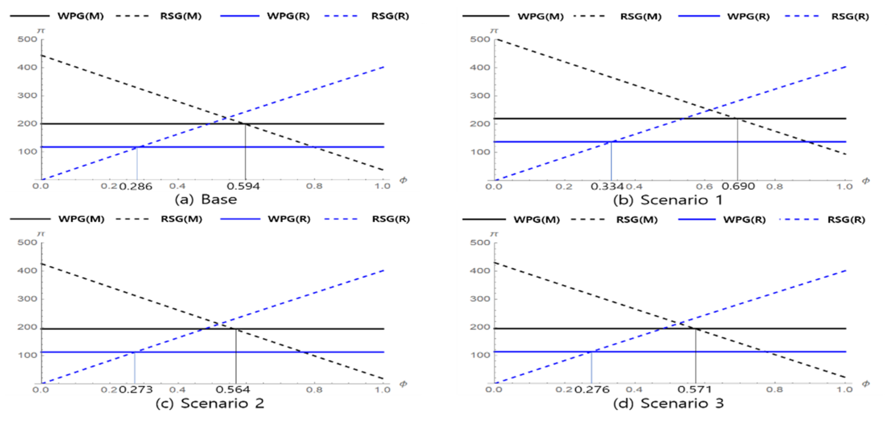
For the retailer, the value of in which the profit increases more than that in the WPG can be obtained, but the form is so complicated that mathematical analysis is difficult. However, a numerical analysis is possible, and we can examine whether there is an interval in which the profits of the manufacturer and retailer increase more than those in the WPG. The basic values are . We can thus create four scenarios according to (see Table 3).
Figure 2 illustrates the results. All of the scenarios have an interval in which the profits of both the manufacturer and the retailer increase at the same time. In Scenario (1) in Figure 2b, the interval in which the profits of both members increase has shifted slightly to the right. This fact indicates that, if the value of the recyclable products increases, the retailer’s distribution ratio must also increase. In Scenarios (2) and (3) in Figure 2c,d, the interval has shifted slightly to the left, indicating that, if the price of the recyclable products or the recycling cost increases, the manufacturer’s distribution ratio must also increase.
In conclusion, if the manufacturer and retailer implement the RSC, the profit of the recycling company also increases, which results in a higher collection rate. Moreover, the product greening improvement level increases with the manufacturer’s profit, and there is a distribution ratio at which the profits of both the manufacturer and the retailer increase simultaneously. This finding indicates that an RSC may be an alternative to a wholesale price contract under the EPR.
5. Numerical Analysis
This section presents the result of a numerical analysis carried out in order to reinforce the abovementioned analysis results. Due to the lack of real supply chain data in Korea, we set the , , , , and by reference to the literature [6,19]. The other parameters are set to represent perfect coordination from the government’s perspective, as shown in Section 4.2, and since there is no reward in reality, the mandatory standard rate ( is set high in order to minimize the reward effect. The assumed parameter values are as follows: . In addition, we examine the changes in environmental and economic performance by substituting the values of in various ways.
5.1. Collection Rate
Table 4 shows the results of the numerical analysis of the collection rate of the recyclable resources. All of the results are rounded to three decimal places.
The collection rate is the highest in the RSG, followed by the CM, WPG, and WP. In the basic numerical example, the collection rates are the same in the CM and WPG. In particular, in all of the cases, the collection rate is higher in the RSG than in the CM. This finding indicates that, if an RSC is implemented under government legislation in the supply chain, environmental performance above the government’s expectations can be achieved. Furthermore, the government’s establishment of incentives to implement the RSC in the supply chain may be a good alternative to improve the environmental performance of the CLSC. This may be because the profits of both the recycling company and the manufacturer increase in the RSC, and thus, the recycling company’s collection efforts and the manufacturer’s power to pay the subsidy both increase simultaneously.
If the value of the recyclable resources increases, so does the collection rate in all of the models, and the collection rate in the WPG then becomes lower than that in the CM. The net worth of the recyclable resources goes to the entire supply chain in the CM, whereas it only goes to the manufacturer in the dispersed model. Thus, the structure has a tradeoff in which the manufacturer must sacrifice its profits to pay the subsidy. Therefore, the incentive to increase the collection rate becomes lower than that in the CM, and the increase in value lowers the rise in the collection rate compared with its effect in the CM.
If the price of the recyclable resources increases, there is no change in the collection rate in the CM, an increase in the WP, and a decrease in the other models. Just as when the value increases, the collection rate in the WPG becomes lower than that in the CM. Since there is no change in the net worth of in the CM, there is also no change in the collection rate. In the WP, the recycling company collects wasted materials on its own, without receiving a subsidy, and thus increases its collection if the price increases. In the other models, the net worth per unit of recyclable resources decreases, and thus, the manufacturer reduces the subsidy while bearing the penalty, which is why the collection rate decreases; this results in a lower collection rate than in the CM.
If the recycling cost increases, the collection rate declines in all of the models. This may be because the recycling company has less power to collect, as its profits per unit decrease. However, the collection rate in the WPG is higher than that in the CM. This is because the net worth of the recyclable resources decreases in the CM, and thus the collection rate decreases, whereas the net worth obtained by the manufacturer in the WPG is unchanged, and the penalty increases when the collection rate declines. Thus, the recycling company’s lower power to collect is supplemented by the subsidy increase.
5.2. Product Greening Improvement
Table 5 summarizes the results of the numerical analysis of the changes in the product greening improvement level. All of the results are rounded to three decimal places.
The product greening improvement level is the highest in the CM, followed by the RSG, WPG, and WP. However, unlike the collection rate, the product greening improvement level is the highest in the CM, because perfect coordination in terms of the collection rate is not perfect in terms of profits—the manufacturer’s profit decreases, and it thus reduces the investment in the product greening improvement level in line with the decrease in profits.
If the value of the recyclable resources increases, so does the product greening improvement level in all of the models. This is because the value increase helps to increase the manufacturer’s profit. If the price of the recyclable resources increases, the quality does not change in the CM, is maintained and then declines in the WP, and declines in the other models. If increases in the WP, the quality increases if is satisfied in the denominator of Equation (13), and decreases otherwise. This finding indicates that the value of the recyclable resources must be above a certain level in order to contribute to the manufacturer’s profit, and thus, investment in the product greening improvement level must be increased. If the recycling cost increases, the product greening improvement level decreases. This may occur because the manufacturer spends more on the subsidy to increase the collection rate than they do on environment-friendly investments to reduce the penalty.
5.3. Profit
Table 5 shows the results of the analysis of the profit changes of the supply chain members. The manufacturer’s profit is the highest in the RSG, followed by the WP and the WPG, while that of the retailer and recycling company is the highest in the RSG, followed by the WPG and the WP. This finding supports the fact that the manufacturer’s profit may decrease when a strong penalty is applied. Moreover, efficiency in the WPG is lower than that in the WP because the profit of the retailer and recycling company increases slightly, while that of the manufacturer decreases. This result shows that government legislation to improve environmental performance adversely affects the entire supply chain’s economic performance. On the contrary, the RSG shows efficiency close to that in the CM. This finding indicates that the RSG in the CLSC helps all of the members, and can serve as an alternative to increase the supply chain revenues under government legislation. The RSC aims to lower product prices and increase demand by eliminating double marginalization. An increase in demand leads to an increase in recycled materials, which then increases the recycling company’s profits. This resolves the issue of the recycling company not being able to recycle because of a lack of profits, which is a bottleneck in the CLSC. This is suggested by the fact that the recycling company’s profit increased significantly in Table 6. The retailer’s profit also showed a remarkable increase, but this follows the ratio of the revenue sharing, and thus, the profit increase of the manufacturer and retailer can be adjusted by changing this value. In other words, the RSC can build a virtuous cycle for the entire CLSC by increasing the recycling company’s profit and thus producing efficiency close to that in the CM.
If the value of recyclable resources increases, so do the members’ profits in all of the models. This may be because the increased profit of the manufacturer leads to an increased subsidy, and therefore a higher profit for the recycling company, while declining prices and increasing demand increase the recycling company’s profit in all of the models. This is reasonable because the profit per unit increases. The profits of the manufacturer and retailer increase and then decrease in the wholesale price contract, but only decrease in the other models. This pattern is the same as for quality, and the same conditions as for quality can be obtained in Equations (15) and (16). If the recycling cost increases, the revenues of all of the members decrease, because the recycling company cannot collect materials efficiently if costs rise; this finding supports the assumption that the recycling company serves as a bottleneck to the CLSC.
5.4. Subsidy
Table 7 shows the results of the analysis of the subsidy changes. If the value of the recyclable resources increases, so does the subsidy. This may be because the net worth obtained by the manufacturer through the recyclable resources increases, and thus, it induces a higher collection rate by increasing the subsidy. If the price of the recyclable resources increases, the subsidy decreases, in contrast to the case above. From the government’s perspective, it is necessary to make the subsidy compulsory, or to increase the reward–penalty intensity when the price of recyclable resources increases, in order to maintain the collection rate. If the recycling cost increases, so does the subsidy, because the cost increases even when the value of the recyclable resources remains the same, which keeps the recycling company from efficiently collecting such resources. Thus, the manufacturer increases the subsidy in order to maintain the collection rate. This result supports the assumption of the reason for the changes in the collection rate, product greening improvement level, and profits.
The value of the recyclable resources and the recycling cost do not change in the short run. Therefore, the government must ease its subsidy regulations when prices increase and tighten them when they decrease, thereby implementing their policy according to the price of recyclable resources in order to increase the collection rate.
6. Managerial Insights
Given the lack of research between channel management and government policy in CLSC management [15,28], this study investigated supply chain decisions in the three-level CLSC, which includes a manufacturer, a retailer, and a recycling company, under government intervention. Considering the intensity of the reward–penalty and subsidy policy, and the product greening improvement level, we first built a CM, as well as three decentralized models that have different contract structures. Furthermore, we provided a numerical comparison of the economic and environmental performance of the CLSC in recyclable resource-dependent scenarios. These models should help, in practice, to improve collection rates, product greening, economic performance, and environmental sustainability, as described in more detail below.
6.1. Improving the Collection Rate Using the RPM and RSC Approaches
The collection rate of the used products significantly affects their return rate and, thus, participants’ profits [28]. Because of its significant influence, several countries—including China, Korea, and European nations—have begun to implement RPM-type policies in order to improve the collection rate [17]. Our finding that the collection rate in the RSG is higher than that in the CM in various cases suggests two main implications. First, the RPM and subsidy approaches do indeed raise the collection rate and perform as well as the CM when an appropriate penalty is imposed. This finding could be useful for governments which are struggling to ascertain the incentive and/or penalty to apply to CLSCs [15]. Specifically, by understanding the balance between the reward and the penalty, governments can formulate an incentive planning policy in order to improve environmental performance. Second, the RSC approach can even achieve a higher collection rate than that of the CM. Although centralized decisions generally outperform decentralized decisions [23], the profits of the recycling company and manufacturer rise as the recycling company’s collection effort increases and the manufacturer decides to pay the subsidy. The government can thus achieve a desirable collection rate through strategic policy implementation.
6.2. Improving Product Greening Using the RPM and RSC Approaches
As consumers’ green consciousness continues to increase, CLSC members must aim to achieve high product greening through profit and cost sharing [3]. Enhancing product greening significantly influences the market size and operation costs, but managerial guidelines for the ways in which to encourage channel members to make such improvements are lacking. Our findings demonstrate that the product greening improvement level is the highest in the CM because of the manufacturer’s financial conflict of interest. In this circumstance, policymakers can combine RPM and RSC coordination in order to raise the level of the product greening improvement. Using an RSC effectively lowers product prices and increases market demand by eliminating double marginalization. Our analysis revealed that RSCs raise product greening, and that CLSC members (except for the manufacturer) can collectively benefit from such green initiatives. In order to plan for product greening improvements, the government must carefully consider the specified range of resource values and investments for the collection of the recycling company in order to ensure that the manufacturer does not exploit the availabel subsidy in order to increase the collection rate instead of making environment-friendly investments to avoid the penalty.
6.3. Improving Economic Performance Using the RPM and RSC Approaches
The role of RPM and government intervention in the subsidy approach has several financial implications for CLSC members. First, even in three-level CLSCs, achieving the optimal profit from the whole supply chain perspective is difficult because of the decentralized setting. When the government imposes a high penalty as part of its green initiative, the manufacturer’s profit falls as it tries to increase the subsidy effort rather than the product greening improvement effort. On the contrary, the economic performance of the retailer and recycling company rises with an increase in the collection rate and the product greening improvement. In order to mitigate this contradictory situation, our findings demonstrate the benefit of the RSC coordination mechanism. When profit and cost sharing are enabled among the CLSC members, not only does their financial performance improve, but the inefficiencies occurring because of the decentralized environment setting are also alleviated. Hence, governments can encourage CLSC members to participate in RSC-driven green activities in order to raise both environmental sustainability and firms’ financial performance.
6.4. Improving Environmental Sustainability Using CLSC Collaborative Efforts
Both the value of the recyclable resources and the recycling cost play pertinent roles in improving the collection rate and the product greening improvement level. In the numerical analysis, we found that a higher value of recyclable resources and lower recycling costs result in an increased collection rate and higher product greening improvement in all of the models. This finding suggests that, to enhance environmental sustainability, manufacturers should consider recycling when they design their products in order to lower the value and recycling cost. Recycling companies also need to develop new technologies in order to lower their recycling costs, and retailers must be actively involved in these activities too. Hence, to improve the overall environmental performance of three-level CLSCs, firms’ sustainability managers must collaborate with other members in the product development and production planning process.
As means to improve the sustainability of CLSC, Green Procurement (GP) and Green Public Procurement (GPP) are commonly cited. GP considers environmental aspects in the procurement activities of supply chain members [40]. GPP refers to the purchase of environmentally friendly products and services from public institutions, and is a policy approach that improves sustainability [41]. The government plays a vital role in the process of implementing GPP and GP [40]. If the government proposes GPP and GPs to the public and private sectors, and incorporates related policies, the overall sustainability of CLSC is expected to improve. Moreover, the introduction of a Life Cycle Agreement (LCA) is considered necessary as well. An LCA takes an analytic approach in quantifying the overall environmental impact based on the entire process of production, distribution, and disposal, including the consumption of raw materials and energy, and the generation of pollutants and wastes. It is a representative activity that a firm can undertake from an environmental perspective [42]. If a supply chain implements an LCA within its products or services operations, it could effectively contribute to the value of recyclable resources while reducing recycling costs. Therefore, the government should prepare regulatory and policy support measures to implement LCA.
7. Conclusions
This study used game theory to analyze the effects of the EPR on the environmental and economic performance of CLSC, and examined whether an RSC can improve the performances. Its results can be summarized as follows. First, a package combining a reward–penalty and subsidy could enhance environmental performance, but might reduce the economic performance of the entire supply chain, as it lowers the manufacturer’s profit. Furthermore, perfect coordination can be achieved in terms of the collection rate by strengthening the reward–penalty, but this decreases the manufacturer’s profit. Second, using an RSC not only increases the entire supply chain’s profits but also achieves performance beyond perfect coordination in terms of the collection rate. Lastly, increasing the net value of the recyclable resources is important for the improvement of the supply chain’s performance, and any subsidy must be run in line with the prices of the recyclable resources.
This study suffers from some limitations, which can be addressed in future research. First, we assume that the product greening improvement level affects only the product demand and manufacturing costs. However, it may also affect recycling costs, or the value of the recyclable resources in some cases. The research models presented in this paper could be expanded in light of this fact. Moreover, we assumed that the prices of recyclable resources are a given, because they are affected by international raw material prices. However, depending on the types of the recycled resources, this may not be the case. Therefore, future studies should aim to extend the model to include the recycling company becoming the price setter. Finally, a numerical experiment using actual supply chain data could provide more specific implications.
Author Contributions
Conceptualization, S.K. and S.P.; methodology, S.K.; formal analysis, S.K. and N.S.; writing, S.K. and N.S.; supervision, S.P.; funding acquisition, S.P. All authors have read and agreed to the published version of the manuscript.
Funding
This study was supported by the Institute of Management Research at Seoul National University.
Conflicts of Interest
The authors declare no conflict of interest.
Appendix A. Proof of Proposition
Proof of Proposition 1.
If the Hessian matrix is obtained by dividing Equation (5) into two-system partial derivatives for each choice variable, we obtain:
When the three conditions listed below are satisfied, the Hessian matrix is a negative definite, and Equation (5) has a joint concavity for the selected variable.
The response curves are obtained by dividing Equation (5) by a one-system partial differentiation for each selection variable. The following results are obtained:
By substituting Equation (A6) into (A7) and (A7) into (A6), assigning the result to (A5), and re-assigning the final results, the result of Proposition 1 can be obtained. □
Proof of Proposition 2.
When Equations (2)–(4) are a two-system partial differentiation for each choice variable, then Equations (2)–(4) are concave when the following conditions are satisfied:
The following reaction curves can be obtained by summarizing Equations (3) and (4) with one-system partial differentiation for each choice variable:
By substituting the above results into Equation (2), and then taking the first-order partial derivative with respect to w and q, we obtain the following reaction curve:
Substituting Equation (A15) into (A16), and (A16) into (A15), and assigning the result to Equations (A13) and (A14), the result of Proposition 2 can be obtained. □
Proof of Proposition 3.
When Equations (19) and (20) are a two-system partial differentiation for each choice variable, we obtain:
Therefore, Equations (19) and (20) are concave for each choice variable. Equations (19) and (20) can be summarized as one-system partial derivatives for each choice variable in order to obtain the following response curves:
Assuming that m is given after substituting Equations (A19) and (A20) into Equation (18), we can obtain the following response curves by dividing the two systems into w and q:
The results of are obtained by substituting Equation (A24) for (A25), and (A25) for (A24). The corresponding results are then substituted into Equations (A19) and (A20) in order to obtain the rest of the results, with an exception of . The obtained results are substituted into Equation (18), and the optimal solution is obtained by dividing by one system for m, and the following results can be obtained:
The first result of Equation (A26) cannot be used because it is the result of zeroing the cost of the recycling company’s collection. The second result is therefore the optimal subsidy. Substituting into the Equation (18), then dividing it by m for the second system, and substituting for it, gives the following result:
Therefore, is the maximum value.
In addition, is substituted into (A21), (A22), and (A23), and is summarized as follows:
If the above condition is satisfied, Equation (18) has bond concavity for the selected variable under . □
Proof of Proposition 4.
Equations (32) and (33) are summarized by substituting into Equation (33).
Therefore, Equations (32) and (33) are concave for each choice variable. Equations (32) and (33) can be summarized as one-system partial derivatives for each choice variable in order to obtain the following response curves:
If the above result is substituted into Equation (31), the following results are obtained based on a two-system partial derivative for each choice variable:
Equation (31) is concave for the choice variable if the above condition is satisfied.
The optimal solution can be obtained by substituting Equations (A33) and (A34) into Equation (31), and if the corresponding result is substituted into Equations (A33) and (A34), the following results of Proposition 4 can be obtained. □
Proof of Proposition 5.
because >, if is less than 1, then it is always .
Based on this assumption, it is always . □
Proof of Proposition 6.
because , if is less than 1, then it is always . □
Proof of Proposition 7.
because , if the reward–penalty intensity is greater than 0, it is always .
because , if the reward–penalty intensity is greater than 0, it is always . □
Proof of Proposition 8.
Because both of the solutions take values less than 0, when the reward–penalty intensity is greater than 0, it is always .
Here, the second condition is always negative and cannot be established. For the first condition, if is satisfied, it is always negative. Thus, if the value of s satisfies the condition, when the reward–penalty intensity is greater than 0, it is always .
If we find the condition that the above equation is less than 0, we can achieve the same result as Equation (45). In order for both sides of the inequality of to have a real value greater than 0, the following condition must be satisfied:
□
Proof of Proposition 9.
If we find the condition that the above equation becomes 0, we can achieve the same result as Equation (42).
2) By substituting Equations (8) and (46) into Equations (15) and (26), we obtain:
In order for the above equation to have a value larger than 0, the following condition must be satisfied:
Therefore, depending on the assumption, . □
Proof of Proposition 10.
(1) It is possible to obtain the value satisfying , and if the value is set to , we obtain:
When the above equation satisfies , a value greater than 1 will be obtained. Because takes a value between 0 and 1 based on the assumption, it is always .
(2) can be obtained through a similar process to (1); the specific formula is omitted due to the complexity of the form. The value of is between 0 and 1 when is satisfied. Therefore, it can be seen that satisfying exists. □
Proof of Proposition 11.
(1) We can obtain through a process similar to Proposition 1. The value of is greater than 1 when is satisfied. Since takes a value of 0, based on the assumption, it is always .
(2) We can obtain through a process similar to (1). The value of is between 0 and 1 when is satisfied. Therefore, it can be seen that satisfying exists. □
Appendix B. Lemma
Lemma 1.
If the following condition is satisfied,is between 0 and 1:
Proof.
The result can be obtained by using Equation (8) if it is smaller than 1. □
Lemma 2.
If the following condition is satisfied,is between 0 and 1:
Proof.
The result can be obtained by using Equation (13) if it is smaller than 1. □
Lemma 3.
If the following condition is satisfied,is between 0 and 1:
Proof.
The result can be obtained by using Equation (24) if it is smaller than 1. □
Lemma 4.
where
Proof.
The result can be obtained by using Equation (33) if it is smaller than 1. □
References
- Guide, V.D.R.; Van Wassenhove, L.N. OR FORUM—The Evolution of Closed-Loop Supply Chain Research. Oper. Res. 2009, 57, 10–18. [Google Scholar] [CrossRef]
- Smith, S. Analytical Framework for Evaluating the Costs and Benefits of Extended Producer Responsibility Programmes; Organisation for Economic Cooperation and Development: Paris, France, 2005; pp. 51–57. [Google Scholar]
- Ghosh, D.; Shah, J. Supply chain analysis under green sensitive consumer demand and cost sharing contract. Int. J. Prod. Econ. 2015, 164, 319–329. [Google Scholar] [CrossRef]
- El Ouardighi, F. Supply quality management with optimal wholesale price and revenue sharing contracts: A two-stage game approach. Int. J. Prod. Econ. 2014, 156, 260–268. [Google Scholar] [CrossRef]
- Maiti, T.; Giri, B.C. A closed loop supply chain under retail price and product quality dependent demand. J. Manuf. Syst. 2015, 37, 624–637. [Google Scholar] [CrossRef]
- Zerang, E.S.; Taleizadeh, A.A.; Razmi, J. Analytical comparisons in a three-echelon closed-loop supply chain with price and marketing effort-dependent demand: Game theory approaches. Environ. Dev. Sustain. 2018, 20, 451–478. [Google Scholar] [CrossRef]
- Jafari, H.; Hejazi, S.R.; Rasti-Barzoki, M. Sustainable development by waste recycling under a three-echelon supply chain: A game-theoretic approach. J. Clean. Prod. 2017, 142, 2252–2261. [Google Scholar] [CrossRef]
- Huang, M.; Yi, P.; Shi, T.L. Triple recycling channel strategies for remanufacturing of construction machinery in a retailer-dominated closed-loop supply chain. Sustainability 2017, 9, 2167. [Google Scholar] [CrossRef] [Green Version]
- Huang, Y.; Wang, Z. Dual-recycling channel decision in a closed-loop supply chain with cost disruptions. Sustainability 2017, 9, 2004. [Google Scholar] [CrossRef] [Green Version]
- Liu, L.; Wang, Z.; Xu, L.; Hong, X.; Govindan, K. Collection effort and reverse channel choices in a closed-loop supply chain. J. Clean. Prod. 2017, 144, 492–500. [Google Scholar] [CrossRef]
- Modak, N.M.; Modak, N.; Panda, S.; Sana, S.S. Analyzing structure of two-echelon closed-loop supply chain for pricing, quality and recycling management. J. Clean. Prod. 2018, 171, 512–528. [Google Scholar] [CrossRef]
- Savaskan, R.C.; Bhattacharya, S.; Van Wassenhove, L.N. Closed-Loop Supply Chain Models with Product Remanufacturing. Manage. Sci. 2004, 50, 239–252. [Google Scholar] [CrossRef] [Green Version]
- De Giovanni, P. Environmental collaboration in a closed-loop supply chain with a reverse revenue sharing contract. Ann. Oper. Res. 2014, 220, 135–157. [Google Scholar] [CrossRef]
- Choi, T.M.; Li, Y.; Xu, L. Channel leadership, performance and coordination in closed loop supply chains. Int. J. Prod. Econ. 2013, 146, 371–380. [Google Scholar] [CrossRef]
- Han, X.; Wu, H.; Yang, Q.; Shang, J. Collection channel and production decisions in a closed-loop supply chain with remanufacturing cost disruption. Int. J. Prod. Res. 2017, 55, 1147–1167. [Google Scholar] [CrossRef]
- Zheng, B.; Yang, C.; Yang, J.; Zhang, M. Dual-channel closed loop supply chains: Forward channel competition, power structures and coordination. Int. J. Prod. Res. 2017, 55, 3510–3527. [Google Scholar] [CrossRef]
- Taleizadeh, A.A.; Moshtagh, M.S.; Moon, I. Pricing, product quality, and collection optimization in a decentralized closed-loop supply chain with different channel structures: Game theoretical approach. J. Clean. Prod. 2018, 189, 406–431. [Google Scholar] [CrossRef]
- Wang, W.; Zhang, Y.; Zhang, K.; Bai, T.; Shang, J. Reward-penalty mechanism for closed-loop supply chains under responsibility-sharing and different power structures. Int. J. Prod. Econ. 2015, 170, 178–190. [Google Scholar] [CrossRef]
- Wang, W.; Fan, L.; Ma, P.; Zhang, P.; Lu, Z. Reward-penalty mechanism in a closed-loop supply chain with sequential manufacturers’ price competition. J. Clean. Prod. 2017, 168, 118–130. [Google Scholar] [CrossRef]
- Wang, W.; Zhang, Y.; Li, Y.; Zhao, X.; Cheng, M. Closed-loop supply chains under reward-penalty mechanism: Retailer collection and asymmetric information. J. Clean. Prod. 2017, 142, 3938–3955. [Google Scholar] [CrossRef] [Green Version]
- Modak, N.M.; Ghosh, D.K.; Panda, S.; Sana, S.S. Managing green house gas emission cost and pricing policies in a two-echelon supply chain. CIRP J. Manuf. Sci. Technol. 2018, 20, 1–11. [Google Scholar] [CrossRef]
- Saha, S.; Modak, N.M.; Panda, S.; Sana, S.S. Promotional coordination mechanisms with demand dependent on price and sales efforts. J. Ind. Prod. Eng. 2019, 36, 13–31. [Google Scholar] [CrossRef]
- Modak, N.M.; Kelle, P. Managing a dual-channel supply chain under price and delivery-time dependent stochastic demand. Eur. J. Oper. Res. 2019, 272, 147–161. [Google Scholar] [CrossRef]
- Almaraj, I.I.; Trafalis, T.B. An integrated multi-echelon robust closed- loop supply chain under imperfect quality production. Int. J. Prod. Econ. 2019, 218, 212–227. [Google Scholar] [CrossRef]
- Zheng, X.X.; Liu, Z.; Li, K.W.; Huang, J.; Chen, J. Cooperative game approaches to coordinating a three-echelon closed-loop supply chain with fairness concerns. Int. J. Prod. Econ. 2019, 212, 92–110. [Google Scholar] [CrossRef]
- He, P.; He, Y.; Xu, H. Channel structure and pricing in a dual-channel closed-loop supply chain with government subsidy. Int. J. Prod. Econ. 2019, 213, 108–123. [Google Scholar] [CrossRef]
- Shankar, R.; Bhattacharyya, S.; Choudhary, A. A decision model for a strategic closed-loop supply chain to reclaim End-of-Life Vehicles. Int. J. Prod. Econ. 2018, 195, 273–286. [Google Scholar] [CrossRef] [Green Version]
- Wang, N.; He, Q.; Jiang, B. Hybrid closed-loop supply chains with competition in recycling and product markets. Int. J. Prod. Econ. 2018, 1–13. [Google Scholar] [CrossRef]
- Alamdar, S.F.; Rabbani, M.; Heydari, J. Pricing, collection, and effort decisions with coordination contracts in a fuzzy, three-level closed-loop supply chain. Exp. Syst. Appl. 2018, 104, 261–276. [Google Scholar] [CrossRef]
- Saha, S.; Modak, N.M.; Panda, S.; Sana, S.S. Managing a retailer’s dual-channel supply chain under price- and delivery time-sensitive demand. J. Model. Manag. 2018, 13, 351–374. [Google Scholar] [CrossRef]
- Gao, J.; Han, H.; Hou, L.; Wang, H. Pricing and effort decisions in a closed-loop supply chain under different channel power structures. J. Clean. Prod. 2016, 112, 2043–2057. [Google Scholar] [CrossRef]
- Modak, N.M.; Panda, S.; Sana, S.S. Two-echelon supply chain coordination among manufacturer and duopolies retailers with recycling facility. Int. J. Adv. Manuf. Technol. 2016, 87, 1531–1546. [Google Scholar] [CrossRef]
- Modak, N.M.; Panda, S.; Sana, S.S. Channel coordination, pricing and replenishment policies in three-echelon dual-channel supply chain. Control Cybern. 2015, 44, 481–518. [Google Scholar]
- Zhang, P.; Xiong, Y.; Xiong, Z.; Yan, W. Designing contracts for a closed-loop supply chain under information asymmetry. Oper. Res. Lett. 2014, 42, 150–155. [Google Scholar] [CrossRef]
- Kim, S.; Park, S. Effects of Supply Chain Contracts on the Profit and Quality Management in a Supply Chain. J. Korean Prod. Oper. Manag. Soc. 2018, 29, 55–75. [Google Scholar]
- Chen, L.; Peng, J.; Liu, Z.; Zhao, R. Pricing and effort decisions for a supply chain with uncertain information. Int. J. Prod. Res. 2017, 55, 264–284. [Google Scholar] [CrossRef]
- Cachon, G.P.; Lariviere, M.A. Supply Chain Coordination with Revenue-Sharing Contracts: Strengths and Limitations. Manag. Sci. 2005, 51, 30–44. [Google Scholar] [CrossRef] [Green Version]
- Chakraborty, T.; Chauhan, S.S.; Vidyarthi, N. Coordination and competition in a common retailer channel: Wholesale price versus revenue-sharing mechanisms. Int. J. Prod. Econ. 2015, 166, 103–118. [Google Scholar] [CrossRef]
- Kim, S.; Shin, N.; Park, S. Effects of Revenue-Sharing Contracts on the Profits of Competing Manufacturers and a Retailer. J. Korean Oper. Res. Manag. Sci. Soc. 2018, 43, 11–35. [Google Scholar] [CrossRef]
- Appolloni, A.; Sun, H.; Jia, F.; Li, X. Green Procurement in the private sector: A state of the art review between 1996 and 2013. J. Clean. Prod. 2014, 85, 122–133. [Google Scholar] [CrossRef]
- Cheng, W.; Appolloni, A.; D’Amato, A.; Zhu, Q. Green Public Procurement, missing concepts and future trends–A critical review. J. Clean. Prod. 2018, 176, 770–784. [Google Scholar] [CrossRef]
- Testa, F.; Nucci, B.; Iraldo, F.; Appolloni, A.; Daddi, T. Removing obstacles to the implementation of LCA among SMEs: A collective strategy for exploiting recycled wool. J. Clean. Prod. 2017, 156, 923–931. [Google Scholar] [CrossRef]
Figure 1.
The CLSC structure.

Figure 2.
Profits of the manufacturer and retailer by scenario.


Table 1.
Summary of recent studies.
| Reference | Supply Chain | Demand Dependence | Performance Measure | Government Participation | ||||||
|---|---|---|---|---|---|---|---|---|---|---|
| Two-Level | Three-Level | Price | Quality | Marketing | Greening Effort | Collection Rate | Profit | Greening Improvement | ||
| [22] | ✓ | ✓ | ✓ | ✓ | ||||||
| [23] | ✓ | ✓ | ✓ | |||||||
| [24] | ✓ | ✓ | ✓ | ✓ | ✓ | ✓ | ||||
| [25] | ✓ | ✓ | ✓ | ✓ | ||||||
| [26] | ✓ | ✓ | ✓ | ✓ | ✓ | |||||
| [27] | ✓ | ✓ | ✓ | ✓ | ✓ | |||||
| [28] | ✓ | ✓ | ✓ | ✓ | ||||||
| [6] | ✓ | ✓ | ✓ | ✓ | ✓ | |||||
| [29] | ✓ | ✓ | ✓ | ✓ | ||||||
| [17] | ✓ | ✓ | ✓ | ✓ | ✓ | ✓ | ||||
| [21] | ✓ | ✓ | ✓ | |||||||
| [30] | ✓ | ✓ | ✓ | |||||||
| [19] | ✓ | ✓ | ✓ | ✓ | ✓ | ✓ | ||||
| [20] | ✓ | ✓ | ✓ | ✓ | ✓ | |||||
| [7] | ✓ | ✓ | ✓ | |||||||
| [8] | ✓ | ✓ | ✓ | ✓ | ||||||
| [9] | ✓ | ✓ | ✓ | ✓ | ||||||
| [10] | ✓ | ✓ | ✓ | |||||||
| [15] | ✓ | ✓ | ✓ | ✓ | ||||||
| [16] | ✓ | ✓ | ✓ | ✓ | ✓ | |||||
| [31] | ✓ | ✓ | ✓ | ✓ | ✓ | |||||
| [32] | ✓ | ✓ | ✓ | ✓ | ||||||
| [5] | ✓ | ✓ | ✓ | ✓ | ✓ | |||||
| [3] | ✓ | ✓ | ✓ | ✓ | ✓ | |||||
| [18] | ✓ | ✓ | ✓ | ✓ | ✓ | |||||
| [33] | ✓ | ✓ | ✓ | ✓ | ||||||
| [13] | ✓ | ✓ | ✓ | ✓ | ||||||
| [34] | ✓ | ✓ | ✓ | ✓ | ||||||
| [14] | ✓ | ✓ | ✓ | ✓ | ✓ | |||||
| [12] | ✓ | ✓ | ✓ | ✓ | ✓ | |||||
| This study | ✓ | ✓ | ✓ | ✓ | ✓ | ✓ | ✓ | |||
Table 2.
Notations.
| Notation | Meaning |
|---|---|
| Manufacturer | |
| Retailer | |
| Recycling company | |
| Demand | |
| Market size | |
| Sensitivity of demand to the product greening improvement level | |
| Sensitivity of manufacturing cost to the product greening improvement level | |
| Collection rate of recyclable products | |
| Wholesale price | |
| Product greening improvement level | |
| Retail price | |
| Profit per unit of the retailer | |
| Manufacturing cost of the manufacturer | |
| Recycling cost of the recycling company | |
| Value obtained by the manufacturer from using recyclable resources | |
| Price of recyclable resources | |
| Coefficient of investment for the collection of the recycling company |
Table 3.
Numerical examples under various scenarios.
| Base | (1) Value-Driven | (2) Price-Driven | (3) Cost-Driven | |
|---|---|---|---|---|
| 20 | 25 | 20 | 20 | |
| 12 | 12 | 16 | 12 | |
| 7 | 7 | 7 | 10 |
Table 4.
Changes in the collection rate.
| 27 | 15 | 5 | 0.418 | 0.092 | 0.418 | 0.824 |
| 29 | 0.458 | 0.093 | 0.438 | 0.860 | ||
| 31 | 0.499 | 0.093 | 0.457 | 0.895 | ||
| 33 | 0.539 | 0.093 | 0.476 | 0.931 | ||
| 27 | 15 | 5 | 0.418 | 0.092 | 0.418 | 0.824 |
| 17 | 0.418 | 0.111 | 0.409 | 0.806 | ||
| 19 | 0.418 | 0.129 | 0.399 | 0.788 | ||
| 21 | 0.418 | 0.148 | 0.390 | 0.770 | ||
| 27 | 15 | 5 | 0.418 | 0.092 | 0.418 | 0.824 |
| 7 | 0.379 | 0.074 | 0.409 | 0.806 | ||
| 9 | 0.340 | 0.055 | 0.399 | 0.788 | ||
| 11 | 0.301 | 0.037 | 0.389 | 0.770 |
Table 5.
Changes in the product greening improvement level.
| 27 | 15 | 5 | 28.521 | 13.929 | 14.082 | 15.435 |
| 29 | 28.635 | 13.940 | 14.120 | 15.555 | ||
| 31 | 28.759 | 13.952 | 14.161 | 15.684 | ||
| 33 | 28.895 | 13.964 | 14.203 | 15.823 | ||
| 27 | 15 | 5 | 28.521 | 13.929 | 14.082 | 15.435 |
| 17 | 28.521 | 13.929 | 14.064 | 15.378 | ||
| 19 | 28.521 | 13.924 | 14.047 | 15.324 | ||
| 21 | 28.521 | 13.914 | 14.030 | 15.272 | ||
| 27 | 15 | 5 | 28.521 | 13.929 | 14.082 | 15.435 |
| 7 | 28.418 | 13.914 | 14.064 | 15.378 | ||
| 9 | 28.325 | 13.900 | 14.047 | 15.324 | ||
| 11 | 28.243 | 13.886 | 14.030 | 15.272 |
Table 6.
Changes in profits.
| Efficiency | Efficiency | Efficiency | |||||||||||||
|---|---|---|---|---|---|---|---|---|---|---|---|---|---|---|---|
| 27 | 15 | 5 | 50,196.6 | 24,514.1 | 12,416.1 | 51.7 | 0.737 | 22,640.3 | 12,691.8 | 235.6 | 0.709 | 25,649.9 | 22,163.7 | 914.3 | 0.971 |
| 29 | 50,397.0 | 24,534.8 | 12,437.1 | 51.8 | 0.735 | 22,736.8 | 12,760.1 | 247.1 | 0.709 | 25,916.6 | 22,166.7 | 954.0 | 0.973 | ||
| 31 | 50,616.6 | 24,555.5 | 12,458.1 | 51.9 | 0.732 | 22,838.0 | 12,833.2 | 258.8 | 0.710 | 26,199.9 | 22,169.9 | 993.5 | 0.975 | ||
| 33 | 50,855.9 | 24,576.3 | 12,479.3 | 52.0 | 0.730 | 22,943.9 | 12,911.2 | 270.7 | 0.710 | 26,500.0 | 22,173.4 | 1033.1 | 0.977 | ||
| 27 | 15 | 5 | 50,196.6 | 24,514.1 | 12,416.1 | 51.7 | 0.737 | 22,640.3 | 12,691.8 | 235.6 | 0.709 | 25,649.9 | 22,163.7 | 914.3 | 0.971 |
| 17 | 50,196.6 | 24,514.4 | 12,416.1 | 74.5 | 0.737 | 22,593.7 | 12,659.3 | 275.9 | 0.708 | 25,522.8 | 22,162.3 | 1073.3 | 0.971 | ||
| 19 | 50,196.6 | 24,505.8 | 12,407.7 | 101.3 | 0.737 | 22,548.3 | 12,628.1 | 314.0 | 0.707 | 25,399.9 | 22,160.9 | 1224.4 | 0.972 | ||
| 21 | 50,196.6 | 24,489.3 | 12,391.0 | 132.2 | 0.737 | 22,504.0 | 12,597.9 | 349.8 | 0.706 | 25,281.1 | 22,159.6 | 1367.5 | 0.972 | ||
| 27 | 15 | 5 | 50,196.6 | 24,514.1 | 12,416.1 | 51.7 | 0.737 | 22,640.3 | 12,691.8 | 235.6 | 0.709 | 25,649.9 | 22,163.7 | 914.3 | 0.971 |
| 7 | 50,015.1 | 24,489.3 | 12,391.0 | 33.0 | 0.738 | 22,593.7 | 12,659.3 | 183.9 | 0.709 | 25,522.8 | 22,162.3 | 715.6 | 0.968 | ||
| 9 | 49,851.9 | 24,464.5 | 12,366.0 | 18.5 | 0.739 | 22,548.3 | 12,628.1 | 134.6 | 0.708 | 25,399.9 | 22,160.9 | 524.7 | 0.965 | ||
| 11 | 49,706.9 | 24,439.8 | 12,341.0 | 8.2 | 0.740 | 22,504.0 | 12,597.9 | 87.5 | 0.708 | 25,281.1 | 22,159.6 | 341.9 | 0.961 |
Table 7.
Changes in subsidies.
| 27 | 15 | 5 | 4653.27 |
| 29 | 4709.08 | ||
| 31 | 4760.34 | ||
| 33 | 4807.57 | ||
| 27 | 15 | 5 | 4653.27 |
| 17 | 4348.16 | ||
| 19 | 4029.18 | ||
| 21 | 3695.35 | ||
| 27 | 15 | 5 | 4653.27 |
| 7 | 4898.77 | ||
| 9 | 5155.36 | ||
| 11 | 5423.84 |
Publisher’s Note: MDPI stays neutral with regard to jurisdictional claims in published maps and institutional affiliations. |
© 2020 by the authors. Licensee MDPI, Basel, Switzerland. This article is an open access article distributed under the terms and conditions of the Creative Commons Attribution (CC BY) license (http://creativecommons.org/licenses/by/4.0/).
Share and Cite
MDPI and ACS Style
Kim, S.; Shin, N.; Park, S. Closed-Loop Supply Chain Coordination under a Reward–Penalty and a Manufacturer’s Subsidy Policy. Sustainability 2020, 12, 9329. https://0-doi-org.brum.beds.ac.uk/10.3390/su12229329
AMA Style
Kim S, Shin N, Park S. Closed-Loop Supply Chain Coordination under a Reward–Penalty and a Manufacturer’s Subsidy Policy. Sustainability. 2020; 12(22):9329. https://0-doi-org.brum.beds.ac.uk/10.3390/su12229329
Chicago/Turabian StyleKim, Sungki, Nina Shin, and Sangwook Park. 2020. "Closed-Loop Supply Chain Coordination under a Reward–Penalty and a Manufacturer’s Subsidy Policy" Sustainability 12, no. 22: 9329. https://0-doi-org.brum.beds.ac.uk/10.3390/su12229329
Note that from the first issue of 2016, this journal uses article numbers instead of page numbers. See further details here.