Modeling and Predictive Mapping of Soil Organic Carbon Density in a Small-Scale Area Using Geographically Weighted Regression Kriging Approach

Abstract

Different natural environmental variables affect the spatial distribution of soil organic carbon (SOC), which has strong spatial heterogeneity and non-stationarity. Additionally, the soil organic carbon density (SOCD) has strong spatial varying relationships with the environmental factors, and the residuals should keep independent. This is one hard and challenging study in digital soil mapping. This study was designed to explore the different impacts of natural environmental factors and construct spatial prediction models of SOC in the junction region (with an area of 2130.37 km²) between Enshi City and Yidu City, Hubei Province, China. Multiple spatial interpolation models, such as stepwise linear regression (STR), geographically weighted regression (GWR), regression kriging (RK), and geographically weighted regression kriging (GWRK), were built using different natural environmental variables (e.g., terrain, environmental, and human factors) as auxiliary variables. The goodness of fit (R²), root mean square error, and improving accuracy were used to evaluate the predicted results of the spatial interpolation models. Results from Pearson correlation coefficient analysis and STR showed that SOCD was strongly correlated with elevation, topographic position index (TPI), topographic wetness index (TWI), slope, and normalized difference vegetation index (NDVI). GWRK had the highest simulation accuracy, followed by RK, whereas STR was the weakest. A theoretical scientific basis is, therefore, provided for exploring the relationship between SOCD and the corresponding environmental variables as well as for modeling and estimating the regional soil carbon pool.

1. Introduction

Soil organic carbon (SOC) plays an important role in soil productivity and the global carbon cycle [1]. SOC stock is not only related to soil, ecosystem, and land-use types, but it also depends on the amount of net biological input, farming methods, organic carbon stability, and many other factors [2,3,4]. The change in SOC directly impacts CO₂ concentration, which then influences solar heat absorption and release, consequently affecting global climate change [5]. This interrelated mechanism and balanced relationship plays a vital role in maintaining normal human habits and building a suitable spatial environment. The effect of environmental variables on SOC varies with the changes in geographical locations; regional scales, geographical locations, and variable thresholds and durations influence this effect [6,7]. The spatial distribution of SOC is not smooth because of the complexity, uncertainty, variability, and heterogeneity of the SOC effect factors [8]. Therefore, exploring the spatial distribution of SOC and the effects of different environmental variables in small-scale areas is important. Overcoming the defect of regional differences is also useful in estimating the global SOC pool before a large-scale application in a complex environment.

Thompson and Kolka analyzed various methods of estimating SOC stock and indicated that soil landscape models (SLMs) [9] are widely applied with high simulation precision. Two main methods are applied in the SLMs: the regional interpolation method (e.g., radial basis function, global polynomial, ordinary kriging, kriging, and co-kriging interpolation) and the main regression model (e.g., multivariate linear regression, spatial error, and spatial lag models). These methods consider spatial heterogeneity, instability, and various SOC environmental factors in constructing SOC models [8]. Thus, the SLM technique improves the prediction accuracy of SOC content [9]. Different environmental factors produce varying SOC contributions, leading to prediction inaccuracy. However, the coefficients of these models rarely consider SOC in different spatial scales and landscape patterns. Thus, existing geostatistical or regression approaches cannot accurately reflect the spatial heterogeneity of SOC and SOC impact factors.

Many approaches, such as regression kriging (RK) and geographically weighted regression kriging (GWRK) [10,11,12,13], have been proposed based on the spatial heterogeneity of soil properties and auxiliary variables to overcome the disadvantages of traditional methods. The multiple linear regression (MLR) approach uses auxiliary variables as predictive factors to simulate soil properties and the ordinary kriging (OK) interpolation approach emphasizes the spatial heterogeneity of simulated variables. RK combines the advantages of the two approaches, but also eliminate the disadvantages of MLR, which can easily create larger residuals and ignore the influences of environmental variables on SOC. Therefore, RK can obtain more detailed and accurate predictions [14,15,16]. MLR, a global spatial regression model, considers the overall effect of environmental variables on SOC spatial distribution in the entire study area, but ignores the effect of spatial heterogeneity and instability of environmental variables on SOC in limited areas [8]. The way of embedding spatial locations into regression parameters and using locally weighted least squares method for a pointwise parameter estimate proposed geographically weighted regression (GWR) was based on the idea of local smoothing [12,13]. GWR, as a locally spatial regression model, considers not only the spatial heterogeneity of soil properties, but also the spatial dependence of the effect factors when estimating the spatial distribution of soil properties [13,17]. Similar to the MLR model, the residual problem of GWR affects prediction accuracy. GWRK, which is an improved GWR, considers the uncertainty and randomness of soil properties, eliminates the residual GWR problem, and solves spatial weights consistency of GWR at different locations with the kriging approach, resulting in improved forecasting simulation results [13,14].

Soil organic carbon density (SOCD) was selected as the research object because this parameter is commonly used to estimate SOC storage, and it has the same basic property as SOC. Terrain and environmental variables influence the spatial distribution of small-scale SOCD, and complex environmental conditions exhibit greater influences on SOCD. The junction region between Enshi City and Yidu City, Hubei province in China, was selected as the study area. Spatial fitting approaches (RK and GWRK) were used to simulate the spatial distribution of SOCD by analyzing the influences of different topographic and environmental variables. This study attempts to provide enhanced mathematical models for SOCD simulation algorithm and new ideas for SOCD spatial variability studies by comparing the simulation and prediction accuracies of different SOCD models.

2. Materials and Methods

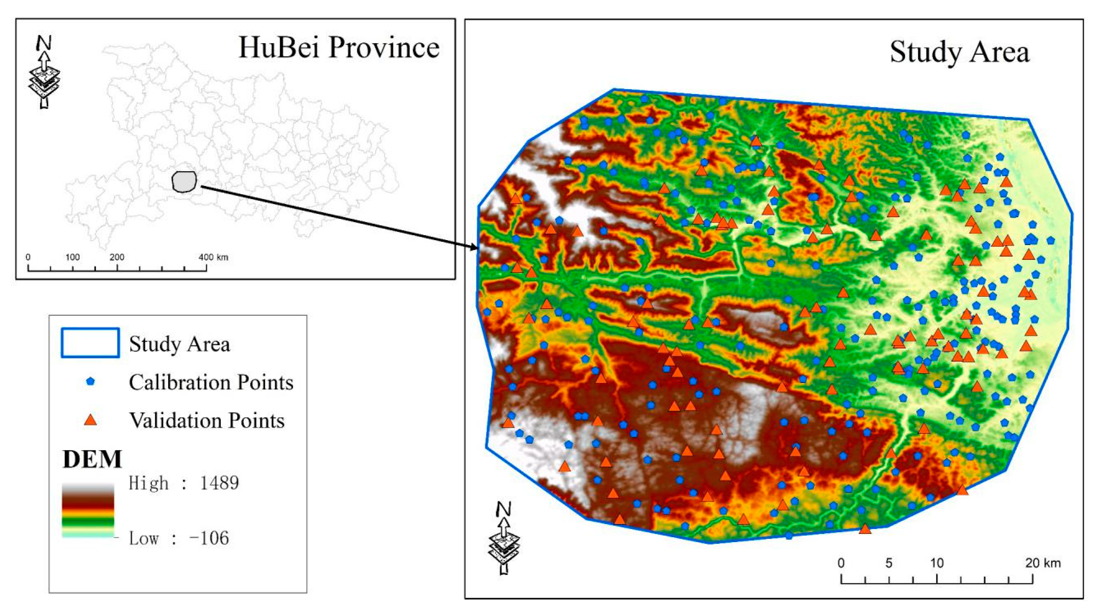
2.1. Study Area

The junction region between Enshi City and Yidu City has an area of 2130.37 km² and is located in the middle reaches of the Yangtze River, China (Figure 1). This region has a northern subtropical climate and belongs to the subtropical monsoon zone, which has high annual rainfall and hills with yellow brown loam, purple soil, lime rock soil, damp soil, and paddy soil. Data from a 1:10,000 scale topographic map and the second soil census data were used, and a representative area with diverse landforms, large topographical changes, and typical soil types was selected. The mesh uniform distribution pattern was adopted with a sampling area of 200 m $\times$ 200 m. A differential global positioning system was used for field sample spatial orientation, and 129 of the 329 samples collected were from plain and arable lands, while the rest were from hilly and uneven terrain regions that have a planting farmland surface 20 cm deep and an orchard planting area 0–30 cm deep, respectively.

2.2. Data Pre-Processing

2.2.1. Soil Organic Carbon Density

The model of SOCD is described as

$${\rho }_{SOC}={\displaystyle \sum }_{i=1}^n\left(1-{\theta }_i\%\right)\times p_i\times C_i\times \frac{T_i}{100}$$

(1)

where ${\rho }_{SOC}$ stands for the SOCD of the soil surface (0–20 cm), i represents the soil horizon (1, 2, 3, …, n), θ_i denotes the gravel concentration (>2 mm) in the ith horizon (volume percentage), p_i represents the soil bulk density in the ith horizon (g·cm⁻³), $C_i$ is the SOC stock (g·kg⁻¹) obtained by multiplying soil organic matter (SOM) content with 0.58 (Bemmelen conversion fraction), and $T_i$ is the soil thickness. Samples in this study were collected from surface soil of 30 cm deep.

2.2.2. Environmental Factors

The terrain attributes were acquired through a digital terrain analysis with the ASTER GDEM v2 with ArcGIS 9.3 (Esri Inc., Redlands, CA, USA, 1999–2006) by 1:50,000 topographic maps and sample information. The obtained terrain indices were the elevation, the slope, the aspect, the surface roughness, the texture, the topographic position index (TPI), the stream power index (SPI), and the topographic wetness index (TWI). The vegetation indices were extracted from the Landsat 8 OLI image (LC08_L1TP_125039_20180929_20181009_01_T1) including the normalized difference vegetation index (NDVI), the blue normalized difference vegetation index (BNDVI), the difference vegetation index (DVI), the green normalized difference vegetation index (GNDVI), and the transformed vegetation index (TVI). The detailed information of these vegetation indices can be found from the index database (https://www.indexdatabase.de/).

2.3. Methods

First, the Kennard–Stone algorithm was used to divide the 329 soil samples into different datasets: 229 samples for calibration and 100 samples for validation. Then, stepwise linear regression (STR) was used to choose the most suitable environmental factors for constructing the prediction models, and then GWR, RK, and GWRK were used as differential value models to simulate and predict the spatial distribution of small-scale SOCD. Finally, root mean square error (RMSE), goodness of fit (R²), and improving accuracy (PIA) were chosen as evaluation indices to compare the accuracy of the SOCD prediction models.

2.3.1. Geographically Weighted Regression Kriging Model

OK and RK models have already been discussed in previous studies; thus, details regarding the principles and formulae of these approaches are not provided in the current study [10]. GWRK is an extension of the GWR model and explores the effects of topographic factors and environmental variables on the SOC spatial distribution based on the local spatial heterogeneity of independent and dependent variables [14]. GWRK eliminates the residual effects on the accuracy of the model by reviewing the OK interpolation on residual errors. GWR intends to embed spatial locations into regression parameters based on the principle of local smoothing and uses locally weighted least squares method for pointwise parameter estimation. GWR is calculated as follows:

$${\widehat{C}}_{gwr}\left(s_0\right)={\displaystyle \sum }_{k=0}^p{\beta }_k\left(s_0\right)\times X_k\left(s_0\right)$$

(2)

where ${\widehat{C}}_{gwr}\left(s_0\right)$ is the SOCD at the geographical location of $s_0$, $X_k\left(s_0\right)$ is the independent variable of the terrain factor and environmental variable at the geographical location of $s_0$, ${\beta }_k\left(s_0\right)$ is the coefficient of the different independent variables in this model, and p is the total number of soil samples.

Residuals appeared after the simulation of SOCD through GWR, affecting the fitting accuracy of the whole model. OK interpolation was necessary to remove the effects of the residuals from GWR and construct the GWRK model.

$${\widehat{C}}_{gwrk}\left(s_0\right)={\widehat{C}}_{gwr}\left(s_0\right)+{\widehat{\epsilon }}_{ok}\left(s_0\right)$$

(3)

where ${\widehat{C}}_{gwrk}\left(s_0\right)$ is the SOCD value of the sampling point at the location of $s_0$, which was estimated through GWRK; ${\widehat{C}}_{gwr}\left(s_0\right)$ is the SOCD value of the sampling point at the location of $s_0$, which was estimated through GWR; and ${\widehat{\epsilon }}_{ok}\left(s_0\right)$ is the result of using OK to interpolate the differences between the SOCD values simulated through GWR and the measured SOCD values.

2.3.2. Model Validation and Evaluation

The advantages and disadvantages of the different interpolation methods can be tested on the calibration and validation data. The calibration data can be used to construct a statistical model, and it can reflect the spatial distribution of SOCD, whereas validation data can be used to evaluate the accuracy of predictions. The prediction accuracy was evaluated by comparing the R² and RMSE of the measured and predicted values on checkpoints. The RMSE value reflects the valuation sensitivity and extreme effects using the sample data. The smaller the RMSE, the more accurate the prediction.

$$RMSE=\sqrt{\frac{1}{n}{\displaystyle \sum }_{i=1}^n{\left(V_{oi}-V_{pi}\right)}^2}$$

(4)

where $V_{oi}$ is the measured value of SOCD, $V_{pi}$ is the predicted value of SOCD, and n is the number of samples.

The RMSE was considered the evaluation criterion, and the maximal value of RMSE the cardinal number to assess the percentage of PIA between different models. PIA is calculated as:

$$PIA=\frac{RMS{E}_{maximal}-RMS{E}_{evaluated}}{RMS{E}_{maximal}}\times 100\%$$

(5)

where PIA is the abbreviation of the improving accuracy percentage, RMSE_maximal is the maximal value of RMSE, and RMSE_evaluated is the RMSE of the evaluated model.

3. Results

3.1. Descriptive Statistical Analysis

The basic statistics of soil organic matter, SOCD, environmental variables, and variation coefficients are shown in

Table 1. Statistical analyses of soil organic matter and environmental variables.

Variables	Range	Minimum	Maxima	Mean	Standard Deviation	Variation Coefficients	Skewness	Kurtosis
SOM (g/kg)	50.4	5	55.4	22.541	7.128	31.62%	0.319	1.055
SOCD (kg·m−2)	11.152	1.038	12.190	5.081	1.657	32.62%	0.342	0.664
TPI	4.482	−2.565	1.917	−0.410	0.687	167.38%	0.047	0.562
SPI	2.209	0.000	2.209	0.029	0.135	457.28%	13.270	207.431
Texture	17.736	0.000	17.736	3.781	3.399	89.90%	1.196	1.430
Roughness	0.269	1.000	1.269	1.018	0.036	3.51%	4.146	20.635
Slope	37.369	0.657	38.026	8.204	6.675	81.36%	1.852	4.042
TWI	16.624	−18.751	−2.127	−10.778	3.697	34.30%	−0.146	−1.215
Aspect	355.236	4.764	360.000	171.996	100.228	58.27%	0.193	−0.939
Elevation	970.000	37.000	1007.000	279.220	237.666	85.12%	1.180	0.362
BNDVI	0.384	0.047	0.431	0.201	0.061	30.17%	0.015	0.312
DVI	2.117	1.232	3.349	1.901	0.307	16.14%	0.613	1.254
GNDVI	0.376	0.094	0.470	0.269	0.060	22.49%	−0.126	0.043
TVI	0.243	0.777	1.020	0.895	0.040	4.51%	−0.214	−0.103
NDVI	0.436	0.104	0.540	0.303	0.072	23.73%	−0.089	−0.093

SOM: soil organic matter, SOCD: soil organic carbon density, TPI: topographic position index, SPI: stream power index, TWI: topographic wetness index, NDVI: normalized difference vegetation index, BNDVI: blue normalized difference vegetation index, DVI: difference vegetation index, GNDVI: green normalized difference vegetation index, TVI: transformed vegetation index.

. SOCD was selected to explore the SOC spatial distribution features, whereas terrain factors were used to exhibit the effects of various terrain conditions on SOCD. The vegetation indices of NDVI, BNDVI, DVI, GNDVI, and TVI were used to represent the land surface vegetation status. The results of the experimental zone show remarkable differences in the SOM with mean, minimum, and maximum values of 22.541, 5, and 55.4 g·kg⁻¹ as well as a full-pitch range of 50.4 g·kg⁻¹. The mean value of SOCD was 5.081 kg·m⁻² with a range of 11.152 kg·m⁻², implying that SOCD changed remarkably in the study area. The coefficients of variation showed the degree of dispersion in the soil properties and environmental variables: <10%, weak variability; values between 10% and 100%, medium variability; and >100% shows strong variability. The absolute values of TPI and TWI were considered to determine the variability because the mean values of these two indices were negative. TPI and SPI had strong spatial variabilities, indicating a strong degree of dispersion; whereas the SOM, SOCD, texture, slope, TWI, aspect, BNDVI, DVI, GNDVI, and NDVI have the median spatial variations; and others have the weak variability.

3.2. Relationship between SOCD and Environmental Variables

Pearson correlation coefficient (Pearson’s r) is frequently used to measure the relationship between data sets, by checking the linear relationship of the interval variables. The closer a correlation coefficient is to 1 or −1, the stronger the relationship of a correlation. By contrast, the closer a correlation coefficient is to 0, the weaker the relationship. The order of the absolute value of Pearson’s r for the terrain variables was elevation > texture > slope > TPI > roughness > SPI, which shows that these variables have stronger correlations with SOCD than other variables (

Table 2. Pearson correlation coefficients of SOCD and environmental variables.

Variables	SOCD	TPI	SPI	Texture	Roughness	Slope	TWI	Aspect	Elevation	BNDVI	DVI	GNDVI	TVI	NDVI
SOCD	1	−0.165 **	0.114 *	0.166 **	0.148 **	0.164 **	0.103	−0.04	0.256 **	−0.051	−0.142 **	−0.128 *	−0.152 **	−0.151 **
TPI	−0.165 **	1	−0.099	−0.239 **	0.092	0.091	−0.118 *	0.038	−0.147 **	−0.014	0.089	0.065	0.105	0.103
SPI	0.114 *	−0.099	1	0.022	0.072	0.097	0.253 **	0.01	0.148 **	0.049	0.043	0.034	0.036	0.037
Texture	0.166 **	−0.239 **	0.022	1	0.224 **	0.325 **	0.046	−0.023	0.276 **	0.01	−0.008	−0.011	−0.014	−0.013
Roughness	0.148 **	0.092	0.072	0.224 **	1	0.918 **	0.045	0.04	0.240 **	0.026	0.130 *	0.094	0.132*	0.132 *
Slope	0.164 **	0.091	0.097	0.325 **	0.918 **	1	0.052	0.088	0.294 **	0.02	0.112 *	0.073	0.107 *	0.109 *
TWI	0.103	−0.118 *	0.253 **	0.046	0.045	0.052	1	0.119 *	0.055	−0.04	−0.057	−0.066	−0.062	−0.062
Aspect	−0.04	0.038	0.01	−0.023	0.04	0.088	0.119 *	1	0.006	−0.073	−0.031	−0.045	−0.031	−0.031
Elevation	0.256 **	−0.147 **	0.148 **	0.276 **	0.240 **	0.294 **	0.055	0.006	1	0.088	−0.033	−0.008	−0.049	−0.047
BNDVI	−0.051	−0.014	0.049	0.01	0.026	0.02	−0.04	−0.073	0.088	1	0.897 **	0.951 **	0.894 **	0.897 **
DVI	−0.142 **	0.089	0.043	−0.008	0.130*	0.112 *	−0.057	−0.031	−0.033	0.897 **	1	0.973 **	0.983 **	0.988 **
GNDVI	−0.128 *	0.065	0.034	−0.011	0.094	0.073	−0.066	−0.045	−0.008	0.951 **	0.973 **	1	0.984 **	0.984 **
TVI	−0.152 **	0.105	0.036	−0.014	0.132*	0.107 *	−0.062	−0.031	−0.049	0.894 **	0.983 **	0.984 **	1	1.000 **
NDVI	−0.151 **	0.103	0.037	−0.013	0.132*	0.109 *	−0.062	−0.031	−0.047	0.897 **	0.988 **	0.984 **	1.000 **	1

SOCD: soil organic carbon density, TPI: topographic position index, SPI: stream power index, TWI: topographic wetness index, NDVI: normalized difference vegetation index, BNDVI: blue normalized difference vegetation index, DVI: difference vegetation index, GNDVI: green normalized difference vegetation index, TVI: transformed vegetation index, ** significance level <0.01, * significance level <0.05.

). In addition, the vegetation indices of DVI, GNDVI, TVI, and NDVI have significant correlations with SOCD. However, among these vegetation indices, strong correlations existed between them, thus, the multilinearly should be removed when construing the prediction models.

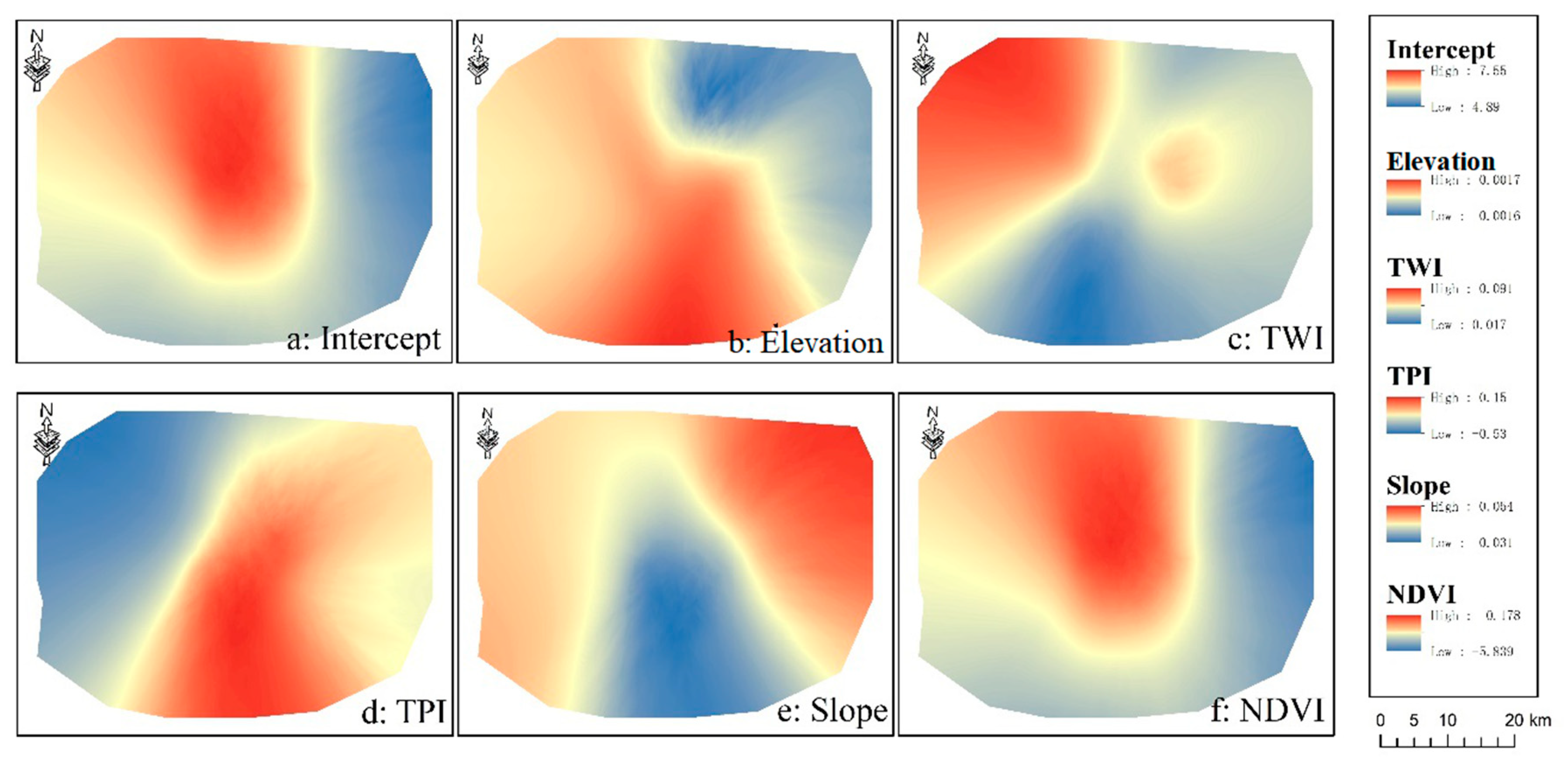
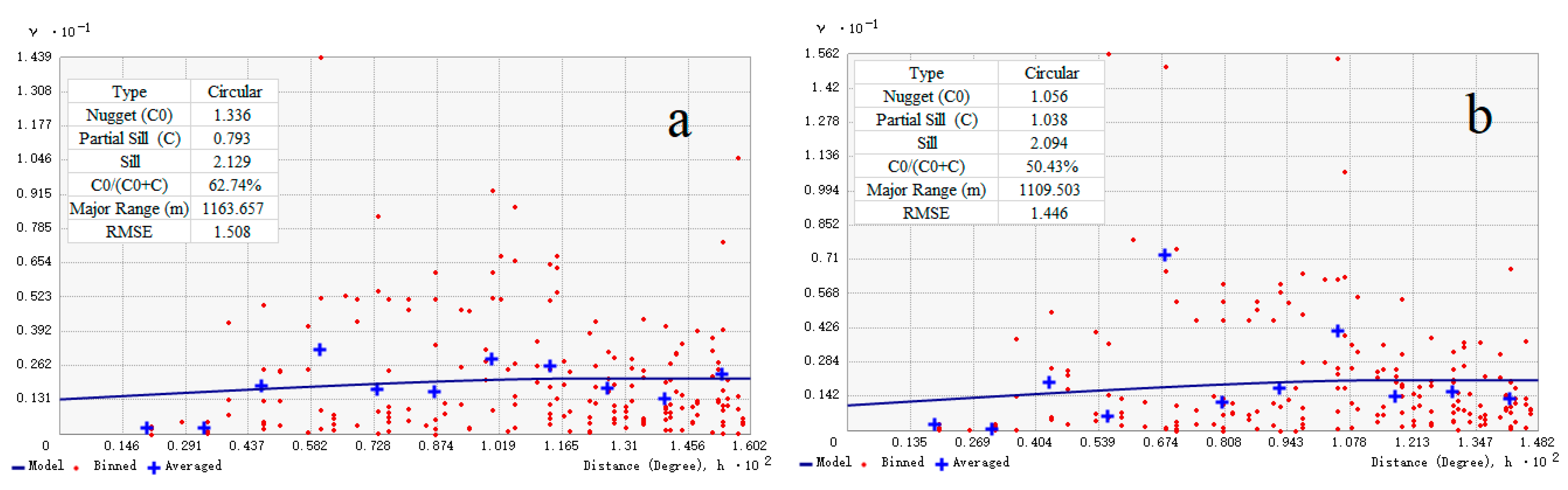
3.3. The Model Parameters of SOCD

The STR model was used to select the most suitable environmental factors for constructing the prediction models, and the TPI, slope, TWI, elevation, and NDVI were used (

Table 3. The parameters of stepwise linear regression (STR) and geographically weighted regression (GWR) when constructing the SOCD models.

STR				GWR
Variable	Coefficient	t-Statistic	VIF	Range	Min	Max	Mean	Std
Intercept	5.881	0.000 *	1.038	2.540	4.960	7.500	6.069	0.726
TPI	−0.364	0.009 *	1.07	0.660	−0.520	0.150	−0.186	0.171
Slope	0.032	0.033 *	1.177	0.080	−0.030	0.050	0.017	0.021
TWI	0.056	0.029 *	1.026	0.070	0.020	0.090	0.052	0.017
Elevation	0.001	0.026 *	1.178	0.000	−0.0016	0.0017	0.001	0.001
NDVI	−2.721	0.041 *	1.032	5.460	−5.730	−0.270	−2.334	1.487

TPI: topographic position index, TWI: topographic wetness index, NDVI: normalized difference vegetation index, * significance level < 0.05.

). The different weighting coefficients indicated the contributions of different factors to SOCD, which showed that the effect of NDVI on SOCD was the most significant, with a weighting coefficient of −2.721. Negative correlations were observed between TPI, NDVI, and SOCD. The higher the NDVI, the more vegetation was covered, and the lower the SOCD. Positive correlations existed between the elevation, slope, and TWI with SOCD. The variance inflation factor (VIF) values were used to check the multicollinearity between these factors, and all of these values were smaller than 7.0; thus, there was no multicollinearity between them. Additionally, t-statistic test was used to check the significance of the environmental factors to SOCD, and these environmental factors went through the t-statistic test.

GWR was used to construct the SOCD prediction models, and the spatial variability relationships between the environmental factors and SOCD are shown in Table 3. The influence weights of TPI ranged from −0.52 to 0.15, and the mean value was −0.186. In addition, the mean coefficient values of other environmental factors were 0.017, 0.052, 0.001, and −2.334 for slope, TWI, elevation, and NDVI, respectively. The spatial distribution characteristics of these factors are shown in Figure 2. The elevation has negative correlations with SOCD in the northeast part of the region, and has positive correlations in the southwest pattern. The TWI has various spatial weights with SOCD in the study region, and the influence degrees were changed with the geographical locations. Other environmental factors also have different influence degrees in the study region. GWR can reflect the spatial distribution characteristics of the weights between the auxiliary variables and SOCD.

The residuals of SOCD are the differences between the measured and predicted values through the STR and GWR approaches. The traditional geostatistical interpolation model, OK, was used to map the residual spatial distribution of SOCD because the sampling points have spatial discontinuity and unsustainability The circular model was chosen for the semivariogram functions, and the detailed information of the model parameters is shown in Figure 3. The nugget values of RK and GWRK were 1.336 and 1.056, and the sill values were 2.129 and 2.094. The ratios of the nugget and sill were 62.74% and 50.43%, respectively, which showed that most of the spatial characteristics of SOCD residuals predicted by STR and GWR cannot be estimated by the semivariogram functions.

3.4. Model Performance

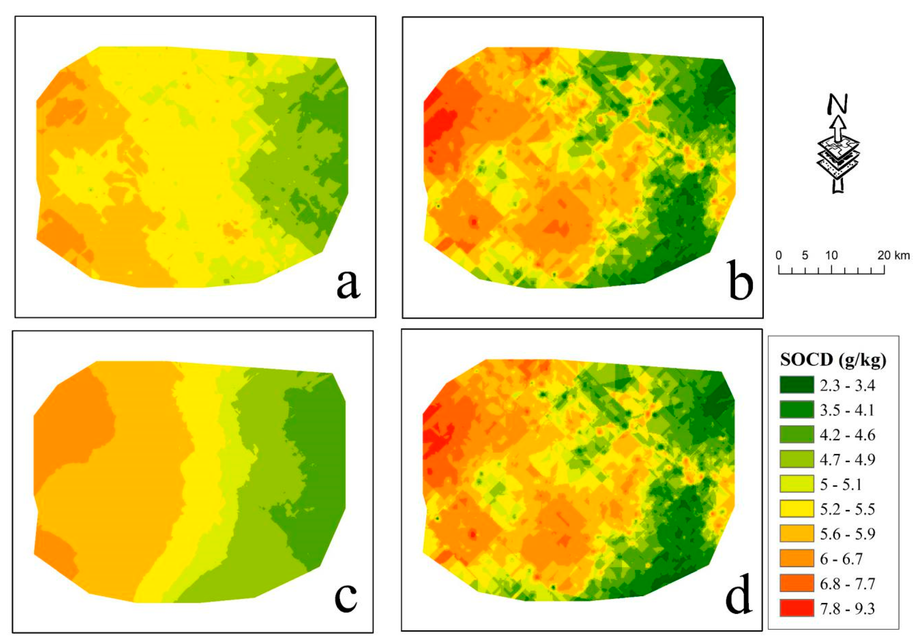
A total of 229 samples were selected as the calibration dataset to build the SOCD models and another 100 samples as the validation data set to test the spatial simulation and prediction abilities of these approaches. R² and RMSE were selected as the evaluation indices.

Table 4. Evaluation indices to test the simulation and prediction accuracy of STR, GWR, RK, and GWRK approaches.

Variables	R2V	RMSEV	PIA
STR	0.105	1.666	0.87%
GWR	0.176	1.603	3.76%
RK	0.151	1.658	0.51%
GWRK	0.192	1.552	6.84%

R²: The goodness of fit, RMSE: root mean square error, PIA: improving accuracy, R²V: R² of validation, RMSEV: RMSE of validation.

shows the predictive accuracy of the testing points in four approaches using the two indices. The validated RMSE of STR, GWR, RK, and GWRK models were 1.666, 1.603, 1.658, and 1.552 kg·m⁻², respectively. These results showed that the values of the GWRK model were smaller than the others, indicating that the GWRK model had the best prediction accuracy and results, followed by GWR, RK, and STR. GWR, RK, and GWRK compared with STR increased by 3.76%, 0.51%, and 6.84%, respectively. The values showed that the prediction accuracy of GWRK compared with STR significantly increased by 6.84%, and the predictive accuracy of GWR and RK were better than that of STR, although their accuracy was less than that of GWRK. Compared with the STR model, GWR highly considered local spatial characteristics of SOCD and its impact factors. Thus, the GWR prediction is more accurate than the STR prediction. RK eliminated the STR residuals of SOCD as much as possible. Meanwhile, GWRK not only considered the local spatial characteristics of the independent and dependent variables, but also eliminated the simulating SOCD residuals. The GWRK simulation and prediction precision was preferred, and the results from the spatial distribution of SOCD through GWRK were more consistent with the actual situation.

3.5. SOCD Maps

The spatial distributions of SOCD based on STR, RK, GWR, and GWRK are shown in Figure 4a–d, respectively. The SOCD ranged from 2.3 to 9.3 g/kg, and the lower values were accumulated in the eastern area of the study region, and the higher values gathered at the western area of the study region. The spatial distribution of SOCD predicted by GWR and STR have line striped features, and the SOCD values increased from the east to the west. The SOCD predicted by GWR was smoother than the SOCD predicted by STR, and there were many irregular patches distributed. In Figure 4b,d, the spatial distribution characteristics of SOCD predicted by RK and GWRK were very trivial relative to STR and GWR. However, the global spatial distribution characteristics have similar distribution trends. From east to west, SOCD values increased.

4. Discussion

The spatial distribution of SOCD had strong spatial heterogeneity and spatial dependence, and the development and evolution of SOCD were influenced by many different environmental factors, so it is important and hard work to accurately map the spatial distribution of SOCD. In this paper, two basal models of stepwise linear regression (STR) and geographically weighted regression (GWR) and two extended models of regression kriging (RK) and geographically weighted regression kriging (GWRK) were used to map the spatial distribution of SOCD. The five environmental factors of elevation, TPI, slope, TWI, and NDVI were used as the auxiliary variables for constructing the prediction models. GWRK is a combination of GWR and OK: GWR is a locally geographical regression model that considers the spatial autocorrelation and dependence between the SOCD and its impact factors and OK is a spatial interpolation model which can be used to reduce the random residuals of regression models. As GWRK has the advantages from GWR and OK, and ignores the deficiencies of them, it had the best evaluation indexes in these four methods: RMSE had the smallest value of 1.552 and the improving accuracy was 6.84% greater than STR. RK is one of the combination methods of STR and OK, although it considers the influences from the environmental factors and reduces the random residuals of regression models. STR is one global regression model and it ignores the spatial characteristics of SOCD and its environmental factors. So, the prediction accuracy of RK was lower than GWRK, but was higher than GWR and STR, and the improving accuracy was 0.51% greater than STR. There were three important points to improve the prediction accuracy of simulation models: the impact factors, the residuals of regression models, and the spatial characteristics of SOCD. It is one important precondition that considers the above three problems to construct the higher prediction accuracy model of SOCD.

SOCD has strong spatial heterogeneity in the study region, and it has spatial varying relationships with the environmental factors. GWR can simulate these relationships and clearly map the spatial distribution of SOCD. The main reason can be due to GWR being a local spatial regression model. The basic assumption of the regression model was that there was no dependency between the environmental factors, and the residuals should be independent in the spatial distribution. Thus, STR can select the suitable environmental factors, and OK can simulate the spatial distribution of the predicted residuals, and these can be removed from the predicted values; then, GWRK and RK can obtain better-predicted values relative to the traditional regression models. Similar research was reported by Zhu and Lin [18], who compared the prediction accuracy between OK and RK to predict soil properties, and the terrain indices and electromagnetic induction surveys were used as the auxiliary variables. The results showed when spatial structure could not be well captured, or when a strong relationship existed between target soil properties and auxiliary variables, RK was more accurate for interpolating soil properties in both landscapes studied, otherwise OK was better. Wang et al. [10] compared GWR and ordinary cokriging (OCK) in predictive mapping of soil total nitrogen (TN) using multiple environmental variables, and the results showed that GWR is a more promising spatial interpolation method compared to OCK in predicting soil TN and potentially other soil properties. Kumar and Lal [19] used GWRK to predict the spatial distribution of SOC based on the other soil properties, and the results showed that the GWRK captures spatial dependent relationships, and addresses spatial non-stationarity issues; hence, this approach improves the estimations of SOC stock. All of these research studies showed that the environmental factors can be used as auxiliary variables, and the spatial geostatistical approaches can be used to predict the soil properties. In these papers, these models (STR, GWR, RK, and GWRK) were used to predict the spatial distribution of SOCD and the differences between these models were compared comprehensively and in detail.

Although GWRK was the best suitable model in estimating the spatial distribution of SOCD in this study area, the variation of environmental factors in other geographical locations may lead to different prediction results and model performance. The limitation and uneven distribution of the soil samples may be also inevitable problems when estimating the spatial distribution of SOCD [20]. Therefore, more studies from different geographical landscapes are strongly encouraged for a better understanding of the spatial relationships between environmental variables and SOCD.

5. Conclusions

The spatial distribution of soil properties has strong interdependence and heterogeneity at different geographical locations with different magnitudes. Previous studies have focused on building spatial interpolation models of soil attributes using traditional geostatistical models. These models consider the spatial heterogeneity and interdependence of soil properties, but ignore the impact of environmental factors on SOCD. The RK, GWR, and GWRK approaches have been successively employed to predict and simulate soil properties because environmental variables, such as topography, climate, and human factors, affect soil properties. These approaches surpass the traditional statistical models. Although the GWR approach considers the regional features of soil properties and various environmental variables, the combination of this approach with the OK approach can compensate for the defect of larger residuals. The spatial distribution of SOCD was modeled and predicted in the present study using four approaches in the same study area. Two evaluation indices were used to test the simulation accuracies of the spatial interpolation models. The results showed that the RMSE of GWRK was minimal, and the prediction accuracy of GWRK was 6.84% higher than that of STR. Therefore, the GWRK model of SOCD can reflect the regional spatial distribution of SOCD and help study the spatial distribution of SOCD. The GWR model aids in implementing the prediction and simulation of SOCD by selecting different environmental factors as auxiliary variables and studying the influences of these variables on SOCD. Additionally, it also provides a theoretical and scientific basis for estimating SOCD in a large area.

References

1. Davidson, E.A.; Janssens, I.A. Temperature sensitivity of soil carbon decomposition and feedbacks to climate change. Nature 2006, 440, 165–173. [Google Scholar] [CrossRef] [PubMed]
2. Choudhury, B.U.; Mohapatra, K.P.; Das, A.; Das, P.T.; Nongkhlaw, L.; Fiyaz, R.A.; Ngachan, S.V.; Hazarika, S.; Rajkhowa, D.J.; Munda, G.C. Spatial variability in distribution of organic carbon stocks in the soils of North East India. Curr. Sci. 2013, 104, 604–614. [Google Scholar]
3. Kumar, S.; Lal, R.; Liu, D.; Rafiq, R. Estimating the spatial distribution of organic carbon density for the soils of Ohio, USA. J. Geogr. Sci. 2013, 23, 280–296. [Google Scholar] [CrossRef]
4. Liu, Z.; Liu, Q. Magnetic properties of two soil profiles from Yan’an, Shaanxi Province and their implications for paleorainfall reconstruction. Sci. China Earth Sci. 2014, 57, 719–728. [Google Scholar] [CrossRef]
5. Stevens, A.; Nocita, M.; Tóth, G.; Montanarella, L.; Van Wesemael, B. Prediction of Soil Organic Carbon at the European Scale by Visible and Near InfraRed Reflectance Spectroscopy. PLoS ONE 2013, 8, e66409. [Google Scholar] [CrossRef] [PubMed]
6. Vasenev, V.; Stoorvogel, J. Urban soil organic carbon and its spatial heterogeneity in comparison with natural and agricultural areas in the Moscow region. Catena 2013, 107, 96–102. [Google Scholar] [CrossRef]
7. Wang, Z.-P.; Han, X.; Chang, S.X.; Wang, B.; Yu, Q.; Hou, L.-Y.; Li, L. Soil organic and inorganic carbon contents under various land uses across a transect of continental steppes in Inner Mongolia. Catena 2013, 109, 110–117. [Google Scholar] [CrossRef]
8. Meersmans, J.; De Ridder, F.; Canters, F.; De Baets, S.; Van Molle, M. A multiple regression approach to assess the spatial distribution of Soil Organic Carbon (SOC) at the regional scale (Flanders, Belgium). Geoderma 2008, 143, 1–13. [Google Scholar] [CrossRef]
9. Thompson, J.A.; Kolka, R.K. Soil Carbon Storage Estimation in a Forested Watershed using Quantitative Soil-Landscape Modeling. Soil Sci. Soc. Am. J. 2005, 69, 1086–1093. [Google Scholar] [CrossRef] [Green Version]
10. Wang, K.; Zhang, C.; Li, W. Predictive mapping of soil total nitrogen at a regional scale: A comparison between geographically weighted regression and cokriging. Appl. Geogr. 2013, 42, 73–85. [Google Scholar] [CrossRef]
11. Szymanowski, M.; Kryza, M. Application of geographically weighted regression for modelling the spatial structure of urban heat island in the city of Wroclaw (SW Poland). Procedia Environ. Sci. 2011, 3, 87–92. [Google Scholar] [CrossRef] [Green Version]
12. Harris, P.; Fotheringham, S.; Crespo, R.; Charlton, M. The Use of Geographically Weighted Regression for Spatial Prediction: An Evaluation of Models Using Simulated Data Sets. Math. Geol. 2010, 42, 657–680. [Google Scholar] [CrossRef]
13. Kumar, S.; Lal, R.; Liu, D. A geographically weighted regression kriging approach for mapping soil organic carbon stock. Geoderma 2012, 189, 627–634. [Google Scholar] [CrossRef]
14. Wang, K.; Zhang, C.; Li, W. Comparison of Geographically Weighted Regression and Regression Kriging for Estimating the Spatial Distribution of Soil Organic Matter. GISci. Remote. Sens. 2012, 49, 915–932. [Google Scholar] [CrossRef]
15. Zhang, C.; Tang, Y.; Xu, X.; Kiely, G. Towards spatial geochemical modelling: Use of geographically weighted regression for mapping soil organic carbon contents in Ireland. Appl. Geochem. 2011, 26, 1239–1248. [Google Scholar] [CrossRef]
16. Szymanowski, M.; Kryza, M. Local regression models for spatial interpolation of urban heat island—An example from Wrocław, SW Poland. Theor. Appl. Clim. 2012, 108, 53–71. [Google Scholar] [CrossRef] [Green Version]
17. Keser, S.; Duzgun, S.; Aksoy, A. Application of spatial and non-spatial data analysis in determination of the factors that impact municipal solid waste generation rates in Turkey. Waste Manag. 2012, 32, 359–371. [Google Scholar] [CrossRef] [PubMed]
18. Zhu, Q.; Lin, H. Comparing Ordinary Kriging and Regression Kriging for Soil Properties in Contrasting Landscapes. Pedosphere 2010, 20, 594–606. [Google Scholar] [CrossRef]
19. Kumar, S.; Lal, R. Mapping the organic carbon stocks of surface soils using local spatial interpolator. J. Environ. Monit. 2011, 13, 3128–3135. [Google Scholar] [CrossRef] [PubMed]
20. Li, J. Spatial Patterns of Soil Organic Carbon Distribution in Canadian Forest Regions: An Eco-Region Based Exploratory Analysis. Master’s Thesis, University of Waterloo, Waterloo, ON, Canada, 2013. [Google Scholar]
Figure 1. Study area and distribution of sampling points (n = 329) across Honghuatao Town.
Sustainability 12 09330 g001
Figure 2. Spatial distribution of explanatory variable coefficients in the geographical weighted regression (GWR) model. TPI: topographic position index, TWI: topographic wetness index, NDVI: normalized difference vegetation index.
Sustainability 12 09330 g002
Figure 3. The model parameters of semivariogram functions for (a) constructing regression kriging (RK) and (b) geographically weighted regression kriging (GWRK).
Sustainability 12 09330 g003
Figure 4. Simulation of SOCD spatial distribution based on the STR (a), RK (b), GWR (c), and GWRK (d) approaches.
Sustainability 12 09330 g004