SRide: An Online System for Multi-Hop Ridesharing


Department of Computer Science, Prince Sultan University, P.O. Box 66833, Riyadh 11586, Saudi Arabia
*
Author to whom correspondence should be addressed.
Sustainability 2020, 12(22), 9633; https://0-doi-org.brum.beds.ac.uk/10.3390/su12229633
Submission received: 14 October 2020
/
Revised: 15 November 2020
/
Accepted: 16 November 2020
/
Published: 18 November 2020
(This article belongs to the Section Sustainable Transportation)
Abstract
:In the context of smart cities, ridesharing in urban areas is gaining researchers’ interest and is considered to be a sustainable transportation solution. In this paper, we present SRide (Shared Ride), a multi-hop ridesharing system as a mode of sustainable transportation. Multi-hop ridesharing is a type of ridesharing in which a rider travels in multiple hops to reach a destination, transferring from one driver to another between hops. The key problem in multi-hop ridesharing is to find an optimal itinerary or route plan for a rider from an origin to a destination in a dynamic, online setting. SRide adopts a novel approach to finding itineraries for riders suited to the online nature of the problem. The system represents ride offers as a time-dependent directed graph and finds itineraries dynamically by updating the graph incrementally and decrementally as ride offers are updated in the system. The system’s distinguishing feature is its incremental and decremental operation, which is enabled by employing dynamic single-source shortest-path algorithms. We conducted two extensive simulation studies to evaluate its performance. Metrics, including the matching rate, savings in total system-wide vehicle-miles, and total system-wide driving times were measured. In the first study, SRide’s dynamic update algorithms were compared with their non-dynamic versions. Results show that SRide’s algorithms run up to thirteen times faster than their non-dynamic versions. In the second study, we used data from the travel demand model for metropolitan Atlanta in the US state of Georgia, to assess the benefits of multi-hop ridesharing. Results show that matching rates increase up to 68%, saving in total system-wide vehicle-miles of up to 12%, and reduction in the total system-wide driving time of up to 12.86% is achieved.
1. Introduction
Online ride-hailing services are becoming increasingly popular in metropolitan areas around the globe. A major drawback of these services is that they add vehicles to the roads and worsen traffic congestion in already traffic-congested areas, negatively affecting the environment and sustainability goals. Ridesharing is regarded as an effective approach to reducing traffic congestion on the roads [1,2,3]. Ridesharing has been shown to improve road network efficiency, which leads to shorter travel times and lower travel costs, without requiring heavy investment in new infrastructure [4,5].
Dynamic ridesharing refers to the mode of transportation in which individual travelers share a vehicle and/or trip costs with other travelers having similar itineraries and schedules. One of the key problems in dynamic ridesharing is matching drivers offering trips to riders requesting trips in real-time [6,7,8]. The matching is performed through an automated system provided by an online matching agency. It is often hard to find a single driver offering a trip with an itinerary close to that requested by a rider. In this situation, riders end up not finding a match. Multi-hop ridesharing attempts to mitigate this problem. In multi-hop ridesharing, a rider could be matched to and travel with more than one driver (Example 2, Section 2.2). At any one time, a rider travels with one driver, but along the route s/he transfers between drivers to reach his/her final destination, similar to multi-hop flights [8].
Multi-hop ridesharing, as a concept, has been around for quite some time now. In the year 2008, Gruebele [9] first conceptualized a real-time multi-hop ridesharing system, without modelling or implementing such a system. Before this, the idea was introduced in dial-a-ride and pick-up-and-delivery systems [10]. There is ongoing research in the area, but there still are no operational multi-hop ridesharing platforms, like, Uber or Lyft. Multi-hop ridesharing has the potential to increase the matching rate in ridesharing systems. Teubner in [11] has studied the economics of multi-hop ridesharing and states: “Multi-hop ridesharing… has the potential to greatly increase the ride availability and city connectedness, especially under high-reliability requirements”. A drawback with multi-hop ridesharing is the inconvenience of transferring from one driver to another.
Various approaches to multi-hop ridesharing have been proposed. These include formulating multi-hop ridesharing as an optimization problem minimizing travel costs, travel times, and the number of transfers in riders’ routes or as a multi-objective route planning problem [12,13,14]. Multi-hop ridesharing systems, like other dynamic ridesharing systems, are real-time and online. Ride offers and requests get added and removed from the system throughout a day, and the system must continually try to find matches between the two, and the matching must be fast. The approaches reported do not take into consideration the real-time and online nature of the problem. They solve the problem off-line as a batch problem, re-solving each time a new offer or request is added or removed, or re-solving at fixed time intervals. This approach is often computationally costly and may lead to missed matches [12]. We propose an online approach to multi-hop ridesharing. Ride offers and requests are added and removed incrementally and decrementally as they arrive into the system and as they expire, respectively.
We propose SRide, a multi-hop ridesharing system in which drivers offer rides by specifying one or more alternate routes from an origin to a destination. For each route, a sequence of intermediate stops, where a driver is willing to pick up and/or drop-off riders, is also specified. A driver’s trip, therefore, consists of one or more than one leg or connection. Together all the drivers’ trips form a network of connections like a transportation network that can be represented by a time-dependent graph. Matching a rider’s request to drivers’ offers involves finding a route within this network that takes a rider from his/her origin to a destination, within his/her time constraints. The system tries to find the shortest such route for the rider, enabling the rider to arrive at the destination at the earliest. The system does this dynamically, in an incremental/decremental fashion, which is enabled by employing dynamic single-source shortest-path algorithms [15,16]. The system does not search for the shortest routes from scratch every time an offer is added or removed but uses the results of previous unsuccessful searches during updates.
We implemented the proposed ridesharing system, evaluated its performance through event-driven simulations using random synthetic data, and compared it with a system using non-dynamic update algorithms. For problem instances, where the average graph density during the simulation time period was low, the system’s performance was almost identical to its non-dynamic counterpart. However, for problem instances with greater than 7000 trips, the performance improvement is obvious. For instances with 20,000 trips, a ridesharing system with dynamic updates was nine times faster than those with non-dynamic updates.
In another simulation, we assessed the benefits of multi-hop ridesharing over single-rider single-driver ridesharing, in which a rider does not transfer from one driver to another, and drivers make single-hop offers only. For this simulation, we used data from the travel demand model for metropolitan Atlanta in the US state of Georgia, developed by Atlanta Regional Commission [17,18]. We measured performance indicators: (i) matching rate, (ii) total system-wide vehicle miles, (iii) total system-wide driving time (an indicator of fuel consumption and greenhouse gas emissions), and (iv) total system-wide journey times, with varying types of trip offers. It is the ultimate goal of any ridesharing system to increase the number of matches and reduce the total system-wide vehicle miles. It was observed that when drivers take a detour from the shortest routes between origin and destination stops and agree to make stops on the way to pick up and/or drop-off riders, the matching rate increases. Results show that the matching rate increases up to 68%, saving in total system-wide vehicle-miles of up to 12% and reduction in the total system-wide driving time of up to 12.86%, is achieved.
The rest of this paper is organized as follows. Section 2 defines terminology and reviews past work in multi-hop ridesharing and dynamic shortest-path algorithms. Section 3 gives a high-level description of the multi-hop ridesharing system and presents the details of the algorithms underlying the system. Experimental studies conducted are described in Section 4. Section 5 discusses the results and suggests directions for future research and development. The conclusions are presented in Section 6.
2. Background
Dynamic ridesharing is a type of organized ridesharing where the organizer is a matching agency or a service provider that uses automated matching to match riders’ requesting trips to drivers’ offering trips [8]. In dynamic ridesharing, rideshare is pre-arranged on short-notice, which can range from a few minutes to a few hours before departure time, and is a one-time non-recurring trip. Drivers are independent, driving their own vehicles. Here we focus on a sub-category of dynamic ridesharing called multi-hop ridesharing: a rider travels from his/her origin to destination by sharing rides with multiple drivers, transferring from one driver to another along the route [9]. We first define some terms related to ridesharing and multi-hop ridesharing. Next, we review research related to multi-hop ridesharing, and we introduce and review dynamic shortest-path algorithms.
2.1. Basic Ridesharing Terminology
A trip is an instance of travel of a traveler from one geographic location to another using a vehicle. A trip has an origin or a source—a location from where a trip starts, and a destination—another location where the trip ends. A trip-offer or ride-offer is an offer made by a traveler, undertaking a trip, to share his/her vehicle with other travelers during the trip. A trip-request or ride-request is a traveler’s request, without a vehicle at his/her disposal, for rideshare. In ridesharing, travelers who share a vehicle to make their trips are the participants. The traveler who drives the vehicle is called a driver, and traveler(s) who shares the vehicle is (are) called rider(s) or passenger(s).
A ride-offer or a ride-request is announced at a certain time during the day called its announcement time. The earliest departure time and latest departure time are the earliest and latest times participants can start their journey from their origin stop. A participant may start walking to or waiting at a stop before the earliest departure time; this time is called ready to depart time. Similarly, participants may specify the latest arrival time at the destination stop. The difference between the latest arrival time and the latest departure time is the maximum travel time window constraint. The decision about a matching agreement must be made by the latest notification time; that is when participants are finally informed about a successful match and sent the trip itinerary. The latest notification time is earlier than the participants’ latest departure time. The time window available for finding a match for a participant is the time difference between the announcement time and the latest notification time (See Figure 1 below. Ready to depart time is not shown.).
The final rideshare agreement may require a driver to take a detour and deviate from the route s/he planned to follow before the rideshare agreement to pick up and drop-off a rider. A driver’s original route is the route s/he would have followed without ridesharing. The route followed while ridesharing is called the ridesharing route. If either the pickup or the drop-off stop or both do not lie on the driver’s original route, the ridesharing is called detour ridesharing [19].
A driver may share a ride with just one passenger or multiple passengers. Similarly, a rider may complete a trip with one driver or may require the services of multiple drivers to complete a trip, transferring from one driver to another en-route to the trip destination. Agatz in [8] has listed four ridesharing variants based on the number of drivers and riders involved: single driver–single rider, single driver–multiple riders, multiple drivers–single rider, and multiple drivers–multiple riders. The last two of these variants involve multi-hop ridesharing.
2.2. Related Work
2.2.1. Multi-Hop Ridesharing
As is the case with other ridesharing forms, there is ongoing research in multi-hop ridesharing, and various approaches have been reported in the literature. However, the approaches reported do not take into consideration the real-time and online nature of the problem. Gruebele in [9] is one of the first papers that defines the terms and sets the goals of a real-time multi-hop ridesharing system, without modelling or implementing such a system. Agatz et al. in [12] formulate multiple-drivers single-rider ridesharing as an optimization problem without implementing its solution.
Herbawi [13] formulates a multiple-driver single-rider ride-matching problem as a multi-objective route planning problem, minimizing travel costs (i.e., distance), travel time, and the number of drivers in riders’ itineraries. The problem is modelled as a time expanded graph, solved as a batch problem using generalized label correcting algorithm. Also, in [13], a solution to a multiple-driver multiple-rider ride-matching using a genetic algorithm and ant-colony optimization is proposed. Ben Cheikh et al. [20] also present an evolutionary algorithmic approach to solve the multi-hop ridesharing problem.
Drews et al. [14], view the driver offers in a multi-hop ridesharing system as a transportation network and model it as time expanded graph. A* and Dijkstra’s algorithm are used to answer shortest-path queries.
Masoud et al. [21] model a multiple-drivers multiple-riders problem as a binary optimization problem. A rolling-horizon approach is followed, and the optimization problem is re-solved at periodic intervals of time, including new trip announcements and excluding the matched trips. Original problem instances take as much as 1600 s to solve, but with pre-processing and employing decomposition techniques, the solution time improves to 400 s.
Coltin et al. [22] describe three different approaches to ridesharing with transfers: a greedy approach, an auction-based approach, and a graph-based approach. The graph-based approach employs the Bellman–Ford algorithm to find the shortest paths with transfers. The experimental results reported provide the cost of solving a problem with 20 vehicles and 18 passengers as 484.7 s, which is unacceptable in a real-time setting.
The real-time and online nature of ridesharing and the need to evaluate ridesharing algorithms in such a setting have been recognized in other ridesharing variants. Alonso-Mora et al. [23] present an ILP-based algorithm that dynamically generates optimal routes for online ride requests in the context of single-driver multiple-rider carpooling, with requests being assigned to dedicated vehicles. The proposed approach performs “batch assignments within a short time span, for example, every 30 s, to the fleet of vehicles”. However, every invocation of the ILP-based algorithm for batch assignment starts with previous assignments.
Chen et al. [24] and Chen et al. [25] discuss multi-hop ridesharing in the context of package delivery. Arslan et al. [26] describe a system for package delivery that uses ad-hoc and dedicated drivers. Cortes et al. [10] model the pickup and delivery problem with transfers as an optimization problem and propose a branch-and-cut solution method. Singh et al. [27] use reinforcement learning to optimally dispatch dedicated vehicles to areas of high future demand in a ridesharing region. There is also ridesharing research being reported in the database community, for example, [28].
In conclusion, the research reported in the literature on multi-hop ridesharing, firstly, does not deal with the online aspect of the problem. The matching problem is solved in a batch mode and in an off-line manner. The behaviour of the solution techniques in an interactive setting, where there are frequent updates, has not been studied. Secondly, there is no computational study on the benefits of multi-hop ridesharing over single-hop ridesharing, reporting quantitative data. This paper attempts to fill these gaps in the research on multi-hop ridesharing.
2.2.2. Dynamic Single-Source Shortest-Path Algorithms
We employ dynamic single-source shortest-path algorithms to dynamically determine the shortest itineraries for ride requests and in the process match riders to drivers. The dynamic shortest-path problem is about re-computing shortest-paths in a graph after a minor change to the graph. The change could be: change in the source node, insertion or deletion of nodes, insertion or deletion of edges, or changes in the weight of one or more edges. Instead of re-computing the shortest paths from scratch, algorithms for dynamic shortest-path problem save computation time by reusing the information already computed before the changes.
There is a large body of research on dynamic shortest path problems. Ferone et al. [29] give a recent survey on the problems. The dynamic version of all pairs shortest-path problem is, for example, dealt within [30] and single-source shortest-path in [31]. Some of the algorithms reported in the literature are fully-dynamic–supporting edge insertion and deletion or edge weight increase and decrease, while some are semi-dynamic, supporting one of the two operations. Some of the algorithms can handle a single edge update at a time, while others can handle a batch of updates [32]. The algorithms have been theoretically analysed, and usually, the computational cost of the dynamic algorithm is measured in terms of the number of updates to output information for an input change [16,33,34,35]. Experimental studies have been conducted to determine the performance of the algorithms in practice [15].
We have adapted the algorithms of Ramalingam et al. [16] to make dynamic changes (i.e., edge insertions and deletions) to a time-dependent directed graph of trip offers maintained by the ridesharing system. Although there are algorithms with better theoretical bounds, the performance of Ramalingam’s algorithms is better than most in practice [15]
The algorithm for edge insertion is a special case of edge weight decrease. The edge weight decrease from +∞ to a certain value is equivalent to an edge insertion. The edge insertion algorithm’s idea is to identify a set Q of nodes whose original shortest-path from the source did not include the newly inserted edge e but does so after the insertion. Changes are now applied to only the nodes in Q, and the changes can be changes in the distance labels, incoming or outgoing arcs of a node. The nodes in Q are then inserted in a heap for further propagation of updated values.
The algorithm for edge removal is a special case of edge weight increase. An edge weight increase to +∞ is equivalent to an edge removal. The idea behind the edge removal algorithm is to identify a set Q of nodes affected by removing an edge e in the shortest path tree. These are the nodes that have the e as an edge in their shortest-path from the source. Changes are now applied to only the nodes in Q, and these nodes are inserted in a heap for further propagation of updated values.
Complexity. Ramalingam’s update algorithms run in time O(ma + na + na log na), where na (i.e., |Q|) is the number of nodes affected by the update and ma is the number of edges having at least one vertex in the affected set [34]. The worst-case time of the algorithms is the same as that of Dijkstra’s algorithm: O(m + n log n), where m is the total number of edges in the graph, and n is the number of nodes.
2.3. Research Contributions
The paper makes two contributions to the research in multi-hop ridesharing. Firstly, we develop a multi-hop ridesharing system, SRide, that operates in an incremental/decremental fashion, unlike the systems reported in the literature that operate in off-line, batch mode. Our system uses dynamic single-source shortest-path algorithms [15,16] to achieve this. It maintains a time-dependent directed graph of trip offers, in which algorithms search for shortest paths from source to destination stops of ride-requests. It also maintains, for each unmatched request, the results of the previous unsuccessful search as a shortest-path tree. It is this tree for each request that is updated incrementally as few ride offers become available, and updated decrementally as ride-offers expire and are removed from the system. We compared the performance of SRide with a system performing non-dynamic updates. Sride, with dynamic updates, was up to nine times faster than the one performing non-dynamic updates.
Secondly, we assess the benefits of multi-hop ridesharing over single-rider single-driver ridesharing, in which a rider does not transfer from one driver to another, and drivers make single-hop offers only. We measured performance indicators: (i) matching rate, (ii) total system-wide vehicle miles, (iii) total system-wide driving time (an indicator of fuel consumption and greenhouse gas emissions), and (iv) total system-wide journey times, with varying types of trip offers. The results of this assessment are discussed in Section 5.
2.4. Multi-Hop Ridesharing: Problem Definition
To define multi-hop ridesharing, we first introduce some notation. Let S be the set of all stops in the ridesharing area, T be the set of ride-offers, and R be the set of ride-requests. In the following definitions, we assume that the latest notification times coincide with the latest departure times for simplicity.
Definition 1.
(Ride Offer) A ride-offer,, from a driver i is a tuple:, whereandare the origin and destination stops,is the announcement time,,are earliest and latest departure times atandis the latest arrival time at, is the capacity of driver i’s vehicle, andis the trip route fromtospecified by the driver.
Trip route of an offer , is the route driver i intends to follow from to , passing through a set of intermediate stops , where the driver is willing to stop to pick up or drop-off a rider. Associated with each intermediate stop , is the latest departure time from the stop, . Travel between any two consecutive stops is a leg or connection of the trip. The trip route is a sequence of stops with their associated times: . The cost of a trip is the time and/or distance traveled via a route from to and is represented as
Example 1.
Figure 2
shows a set of four ride offers as a graph. Offer1 () has stop 2 as its origin, stop 7 as its destination, 7:35 as its announcement time (not shown in the Figure), 7:50 as its earliest and 8:05 as its latest departure times, 8:26 as its arrival time at stop 7, and capacity is 1. It has an intermediate stop 5 with the latest departure time 8:15. As a tuple the offer can be represented as:. Offer 4 is an offer with no intermediate stops and a capacity of 2. The tuple for Offer4 is:.
Definition 2.
(Ride Request) A ride-request,, from rider j is a tuple:, whereis the origin stop,is the announcement time,, are the earliest and latest departure times at, is the destination stop, andis the latest arrival time at the destination.
In single-hop ridesharing, a rider travels with only one driver; there is one pick up for the rider and one drop-off. Single-hop ride-matching involves assigning riders to drivers in such a way to minimize the total cost of the trips: , where is the cost of trip o. Each assignment is subject to the timing and other constraints, such as preference, capacity, etc. The timing constraint is that a rider i can be assigned to a driver j if the rider i is ready to leave before driver j’s latest departure time (i.e.,
In multi-hop ridesharing, a rider travels with more than one driver, transferring from one driver to another at certain stops along the route to reach his/her final destination. The matching process matches each rider to a set of drivers and yields route plans or itineraries for the riders and the drivers: , where is route plan for rider j. A route plan gives the order in which the rider will share rides with the drivers and the pickup and drop-off timings at various stops. Route plan for a rider j, consists of n hops: . Each hop is a journey with driver offering trip , from a stop to a stop , both lying on the driver’s trip route. We represent a hop as a tuple , where is the start–stop of the hop, the departure time from the start–stop, is the end stop of the hop, and is the arrival time at . We reference the components of a tuple by functions, such as, , etc.
The route plan for a ride-request must be spatially and temporally continuous. That is, arrival stop of must be the departure stop of for spatial continuity, and the arrival time of must be less than or equal to the latest departure time of for temporal continuity. Moreover, the origin stops of and and arrival stops of and must be the same [13].
The matching process should find route plans for the maximum number of ride requests, or maximize N in and minimize the total cost of the route plans in . The cost of a route plan is expressed in terms of total driving/journey time, total vehicle miles traveled, and/or the number of transfers or hops in the route plan.
Definition 3.
(Multi-Hop Ride Matching Problem) Given a set of stops S, sets of ride offers T and ride requests R, find route plans for the drivers and riders:, whereis route plan for requestconsisting of n hops:. The set of route plansshould:
Eachshould satisfy the feasibility constraints:
where (1) and (2) are for spatial and temporal continuity, (3) states that the origin stop of the first hop and arrival stop of the last hop should correspond to the origin and arrival stops of the request, and (4) states that first hop should be accessible to the rider j.
Example 2.
Consider a ridesharing system in the state shown in Figure 2, where four ride offers have arrived. Suppose a ride request,, arrives:. A single-hop ridesharing system will fail to find a match for this request, but a multi-hop system will be able to match the request to two offers: offer3 and offer4, with the following two-hop route plan:. The route plan is the earliest arrival plan and enables the rider to reach destination stop 7 at the earliest (i.e., 8:15). An alternative itinerary via stop 5 has an arrival time of 8:26 at stop 7 and is not optimum.
3. Development of SRide
3.1. Incremental/Decremental Approach to Multi-Hop Ridesharing
We can view a ridesharing system’s online operation as an event handler that receives and processes a stream of external events occurring randomly. The two main types of external events must be handled: new ride-offers arriving from the drivers and new ride-requests arriving from riders. Other than these, internal events to remove ride-offers and remove ride-requests arise when matches are found or offers and requests expire. In this section, we describe, at a high level, how the multi-hop ridesharing system handles these events. The details of the algorithms to handle the events are in Section 3.2.
Assumptions. We assume that the set of stops, S, in the area where the matching agency provides ridesharing services is fixed. We assume a stop is not just a geographical point with longitude and latitude but a small region. For example, this could be a square in a city or a block or a parking lot. A rider may walk around in the region to be picked up, and a driver may stop at any point in this region to pick up or drop-off a passenger. The time involved in walking around or driving within a region is not represented explicitly; the algorithms use a driver’s latest departure time from a stop.
To improve the chances of finding a match, we assume that a driver may offer multiple routes from his/her origin to a destination. during the search, all the offered routes are considered. however, when an offered route (or part of it) matches a rider request, we assume the driver commits to following that route; other routes offered by the driver are removed from the trip graph. if no match is found for a driver, we assume the driver follows the shortest offered route to the destination. drivers do not take a detour from the committed route to pick up other “nearby” riders. furthermore, there are no “meeting points”: riders’ do not walk from their origin to another stop, and neither do they walk to their destination stop. this limits flexibility and may reduce the number of matches found, as pointed out in [36]. we also do not implement the feature where a driver changes his/her mind before the start or in the middle of a journey and withdraws his/her ride offer, or a rider cancels his/her matched ride request just before the start of a journey or in the middle of an ongoing journey.
A driver specifies a route in his/her offer by specifying a set of intermediate stops, , between the origin () and destination () stops. At intermediate stops, the driver may pick up and/or drop-off riders. Legs or connections of the route are journeys between two consecutive stops. For each intermediate stop, an approximate latest departure time is specified. The latest departure time depends on the travel distance between consecutive stops; we assume drivers provide the latest departure times from their experience or use an application like google maps to estimate it. The routes of ride-offers are represented as a time-dependent directed graph. Its vertices or nodes are the stops, and edges represent currently active trip connections, i.e., the connections corresponding to the trip legs that are yet to take place. Edge weight or cost is the time of the travel. (See Figure 3 of Example 3 below.)
Ride-request Arrival. Ride-requests announced by the riders are added to the current unsatisfied ride requests, R, in the system. When a new ride request arrives in the system, a time-dependent shortest-path algorithm (Figure 4), searches for the shortest route plan (or an itinerary) from the origin to the destination stop. If a route plan is found, the request is said to have matched the driver(s) along the route. The rider and the driver(s) receive the itinerary from the system, and the request is removed from the set of unsatisfied requests. An itinerary of a successful match for a rider includes information on the scheduled route and the drivers with whom the travel is planned. For the drivers, the itineraries include the schedules to pick up and drop off riders. Otherwise, our incremental approach does not discard the shortest-path tree found during the unsuccessful search but saves it with the request. (See Example 3 below.) In the future, as new connections are added, the shortest-path trees of unsatisfied requests are updated, and new routes may be found.
Example 3.
Figure 3a depicts an example trip graph for three active offers. The latest departure times for each leg are shown, and the arrival times at the destination stops are red. A ride-request, requesting a ride from stop 2 to 8 at 7:55, arrives at 7:40 (announcement time). As is clear from the trip graph, this request cannot be satisfied: there is no connection connecting stop 8. The system’s shortest-path algorithm will search from r’s origin stop, i.e., 2 and trace the shortest path tree, which of course, will not include stop 8. This tree is shown in Figure 3b. The tree is stored with the unsatisfied request r, and future additions of trips will update it, and a route to stop 8 may be found.
Ride-offer Arrival. Ride-offers announced by the drivers are added to the current offers, T, in the system. When a new ride-offer arrives, new edges, corresponding to the new connections, get added to the graph. The system goes over the unsatisfied requests in R, one-by-one, and updates their shortest-path trees incrementally. The updating may result in the discovery of new routes and matching of unsatisfied requests.
Ride-request Removal. A ride-request is removed when it expires or as soon as an itinerary is found for it. A request expires if there are no ride offers that match it before its latest departure time. An expired ride request is simply removed from the system, and no updating is required. (In Example 3, request r is removed just after 8:00 if it is still unsatisfied at this time.)
Ride-offer Removal. A ride-offer does not expire all at once and is not removed in one go. A ride offer expires one leg at a time. A leg or connection expires just after the leg’s departure time. No rider can board the leg after its latest departure time, and the edge corresponding to it must be removed from the graph to prevent it from being considered in future searches. (In Figure 3a, offer 3’s connection from 1 to 3 must be removed just after 7:45, its connection from 3 to 5 must be removed just after 7:57, and so on.) The ride offer as a whole expires when the driver starts the last leg of his journey. A connection must also be removed if there are no vacant seats available in it. This can happen when a ride-request matches an offer, and a seat is allocated to the rider.
When a connection (or an edge) is removed from the graph, the system goes over the unsatisfied requests one by one and updates its shortest-path trees decrementally. In the process, some stops may become unreachable in the shortest-path trees.
3.2. Details of the Underlying Algorithms
We now describe the algorithms underlying SRide in some detail. The algorithms adapt the shortest-path algorithms of Ramalingam et al. [16] for time-dependent directed graphs. The algorithms have been theoretically analysed, and their complexity bounds are given in [34,35]. Buriol et al. [15] describe and evaluate these algorithms and their various specializations for updating shortest-path trees clearly and concisely. The algorithms described in [15] are designed to update shortest-path trees after an edge weight increase or decrease. In the ridesharing system, edges are inserted and removed; edge weights are assumed to be constant throughout its operation.
We first describe the common data structures used by the algorithms. In the subsequent subsections, algorithms to add ride offers and requests and remove ride offers and requests are described.
3.2.1. Data Structures
The ridesharing system’s main data structure is the trip graph that represents the ride offers. The trip graph is searched to find possible itineraries for the ride requests. The graph has a fixed set of stops of the ridesharing system as its vertices or nodes. Its edges are the legs or connections of the ride offers. The graph is a directed graph. Both the outgoing and incoming edges for each node are stored, as the algorithms need access to the incoming and outgoing connections of stops at various points. Therefore adding a new connection to the graph involves adding an outgoing edge at the vertex corresponding to the connection’s departure stop and adding an incoming edge at the vertex corresponding to the connection’s arrival stop. The graph is time-dependent: the outgoing edges active at a vertex depends on the time of the day. An edge corresponding to a connection departing a stop n at 9 am will not be active after 9 am.
A connection is represented by four attributes: departure stop, departure time, arrival stop, and arrival time. A ride-offer stores source stop, destination stop, announcement time, lead time (i.e., the time difference between announcement time and latest departure time), and the trip’s legs or connections. A ride request stores: source stop, destination stop, announcement time, lead time, and departure time. Other than these attributes, two arrays of length equal to the number of stops are used to represent the shortest path tree found for the request (treeSP) and arrival times at various reachable stops (dist). In the array, treeSP, each index corresponds to a node (stop), and it records the parent node’s index. The index corresponding to the source stop, stores minus one (−1) as a special value, indicating that it has no parent. We also use an array representing incoming connections of stops in the shortest-path tree but do not refer to it in the pseudo-codes to simplify descriptions. The source stop has no incoming connection, so its value for the incoming connection is null. The array of incoming connections is used to trace the itinerary when a request is satisfied.
The algorithms use a heap-based priority queue. We use the heap operation names in the pseudo-codes, and their specification is the same as in [16]. We repeat the specification of the operations below.
- size(): returns the number of elements in heap H;
- FindAndDeleteMin(): returns the item in heap H with minimum key and deletes it from H;
- InsertInHeap(u, k): inserts an item u with key k into heap H (In the pseudo-code below, a node object is inserted and u and k are the attributes of the node object);
- AdjustHeap(u, k): if uH, it changes the key of element u in heap H to k and updates H. Otherwise, u is inserted into H.
In the algorithms’ pseudo-code, the dot notation refers to the operations and attributes of the objects.
3.2.2. Adding Ride Requests
After a new ride-request is added to the set of unsatisfied ride requests, the system tries to find a route in the trip graph from the request’s source stop to the destination stop using a time-dependent Dijkstra shortest-path algorithm. The algorithm appears in Figure 4. If a route is found, the request is removed from the system. Otherwise, the shortest-path tree (treeSP) and arrival times vector (dist) computed by the algorithm are saved with the request. Future edge insertions update both these structures. The details are in the following.
The algorithm (Figure 4) inputs the trip graph, G, and the request, req. The algorithm’s output is the shortest path tree, treeSP, and the arrival-time vector, dist. Both these vectors are stored as attributes of req object.
Lines 1 to 3 initialize the vectors dist to −∞ and treeSP to −1. The source stop’s dist value is initialized to the time the rider starts waiting at the source stop, in line 3. A search node is created and inserted in a heap-based priority queue H in line 4.
The algorithm’s main loop from lines 5 to 23 removes in each iteration, the node with the lowest arrival-time value from H, and looks at the outgoing edges (or connections) from the node’s stop curStop. If curStop is the destination stop of the request, the request is marked as “satisfied”. Although the shortest route from the source to destination stop has been found, the search does not stop but continues, and the complete shortest-path tree is traced (It is necessary to have the complete shortest-path tree for a request, for any future updates to work correctly, even if it is satisfied. If two requests match simultaneously and if their shortest-paths share a connection, that can be allocated to only one of them because of a capacity constraint, then one of the two requests must be marked as “unsatisfied” once again and its shortest-path tree updated).
In the inner loop, from lines 12 to 22, outgoing connections of curStop are examined. (See Example 4 below) The condition on line 13 checks if an outgoing connection, c, is accessible at the arrival time of the curStop. If it is, we check if the neighbouring stop (i.e., c’s arrival stop) can be reached earlier through connection c (line 16). If it can be reached earlier, we update the arrival time and parent of the stop (17–18) and create a new search node corresponding to the neighbour and en-queue it in the priority queue H (line 19). In this way, the arrival time values in dist decrease progressively, from the initial value of +∞. The outer loop and the algorithm terminate when the priority queue is empty.
Example 4.
Figure 5 depicts part of a trip graph to illustrate ShortestPath algorithm from lines 12 to 22. Stop 2 is the curStop with three outgoing connections: c1, c2, and c3. A connection’s departure and arrival times are shown. The arrival time at curStop is 8:00. So, connections c1 and c2 are accessible because their departure times are greater than or equal to 8:00. Connection c3 is not accessible. Taking connection c2 will not improve arrival time at stop 3. Stop 3 is already reachable at an earlier time. The node corresponding to stop 5 is the only neighbouring node whose arrival time and parent will change. Its arrival time will change from 8:15 to 8:13, and its new parent will be 2. A node corresponding to stop 5 is created and inserted in the heap.
3.2.3. Adding Ride Offers
After a new ride offer is announced and added to the set of active offers, its legs or connections are added as edges to the trip graph, and the shortest-path trees of waiting requests are updated. The algorithm is given in Figure 6. The tree update algorithm (Figure 7) checks if the new trip’s connections are accessible from the stops of the shortest path tree and if an accessible connection leads to a better arrival-time value at its arrival stop. Departure stops of such connections are inserted in the priority queue, and Dijkstra’s search algorithm is run.
The tree update algorithm, updateShortestPathTreeAfterEdgeAdd, is depicted in Figure 7. Loop from line 1 to 5 examines the connections of the new trip being added. Line 2 checks if a new connection is accessible from the connection’s departure stop and if it improves the current arrival-time value at the connection’s arrival stop. If the connection is accessible and improves the arrival-time value of the arrival stop, there is a better connection to reach the arrival stop; therefore a new node corresponding to the departure stop is created and en-queued in the priority queue (line 3) for further search.
In the iterations of the main loop (lines 6 to 24), the node with the smallest arrival-time value is removed from H, the stop corresponding to the node, curStop, is checked if it is the destination stop, in which case the request is marked as satisfied. Next, the neighbours of curStop, connected through outgoing connections, are examined. If a connection c to a neighbour is accessible and the arrival-time value of the neighbour (i.e., c’s arrival stop) improves by traveling through c, the parent and the arrival time are updated, and a new search node corresponding to it is created and inserted in a heap for further search.
3.2.4. Removing Ride Offers
Just to recall, as the drivers undertake their journeys, the journey’s legs expire one by one and must be removed from the trip graph. The ride offer as a whole expires and must be removed from the set of offers when the driver starts the last leg of his journey. In the following, we describe the algorithms for removing a leg or a connection of a ride-offer from the trip graph and for updating the shortest-path trees.
The top-level procedure, removeTripLeg, is given in Figure 8. Its inputs are the trip graph G, the set of requests R, and the trip leg or connection to be removed, conn. It updates G by removing the edge corresponding to the connection, conn. The loop from lines 2 to 4 updates the shortest-path trees of the unsatisfied requests in R.
The algorithm, updateShortestPathTreeAfterEdgeRmv (Figure 9), updates shortest-path tree of a ride request after a connection is removed. The idea behind the algorithm is to identify a set of affected nodes Q in the shortest-path tree. The part of the shortest-path tree that needs to be updated after the removal is the part that is dependent on the nodes in Q. The rest of the shortest-path tree remains unaffected.
The algorithm first checks if the removed connection is part of the shortest-path tree (line 1). If it is not, the request’s shortest-path tree is unaffected by the removal of the connection, and nothing needs to be updated; the algorithm terminates. Otherwise, the incoming connections of conn’s arrival-stop are examined to see if there is an alternative connection accessible and reach the arrival-stop at the same time as the removed connection (loop in lines 4 to 9). (See Example 5) If such a connection is found, the tree is updated with the new connection (line 6), and the algorithm terminates. If not, the arrival-stop is added as the first node to the set of affected nodes Q. This arrival-stop is the root of the subtree of nodes affected by the removal of conn.
Example 5.
Figure 10 depicts part of a shortest-path tree to illustrate the update algorithm of Figure 9. Connection c1 has just been removed. Loop at line 4, looks at the incoming connections of node 7. These connections are shown dotted because they are not part of the shortest-path tree. Connection c3 has an arrival time at 7 equal to that of c1 and is accessible at stop 5. Therefore update after c1’s removal involves just adding c3 to the tree.
The loop from lines 11 to 27 determines other members of the set of affected nodes, Q. For each node , dist[u] is reset to +∞, and treeSP[u] is reset to −1. In the loop at line 14, the outgoing connections of u are examined one by one. If an outgoing connection, outc, belongs to the shortest-path tree, the incoming connections of outc’s arrival stop, v, are examined to determine if there is an alternative connection to v that is accessible and reaching v at the same time as outc. If such an alternative connection is found, treeSP[v] is updated; otherwise, v is added to the set of affected stops, Q.
It may be possible to reach the nodes in the affected subtree through nodes outside the subtree. This is determined in the loop from lines 28 to 37. The loop again examines the nodes in the affected set. For each node v Q, the incoming connections of v are examined. If an incoming connection, inc, is accessible at inc’s departure stop u and it improves the arrival-time value at inc’s arrival stop, i.e., v (line 31), the values of dist[v] is updated to the better value and so is the value of treeSP[v] (line 32 and 33). If an alternative connection to v is found and v’s arrival-time value improves, the node v is added as a search node to the priority queue (line 36).
Lastly, the loop from lines 38 to 53 is Dijkstra’s main loop. It searches starting from the nodes whose values were updated and it finds paths to nodes currently unreachable. It may be noted that it will not find a path to the destination node because if such a path existed the request would have been satisfied before the removal of the connection.
3.2.5. Removing Ride Requests
A ride request is removed from the system when an itinerary is found for it, or it expires. An expired ride request is simply removed from the system, and no updating is required. The algorithm in Figure 11 shows the steps involved in removing a satisfied ride request. It may be noted that the itinerary legs are removed only if there are no seats left in the vehicle for that leg.
4. Performance Evaluation
We conducted two extensive simulation studies to evaluate the performance of SRide. In the first study, we assessed the performance of the algorithms underlying the system by measuring their execution time. In the second study, the benefits of multi-hop ridesharing over single-hop ridesharing were assessed. We measured the performance indicators, matching rate, system-wide total vehicle miles traveled, system-wide total driving time, and system-wide total journey time. In both the studies, the simulations were event-driven: the ridesharing system processed a train of ride-offer and ride-request events arriving into the system, simulating the real-world scenario. The first study used randomly generated data, while in the second simulation data from Atlanta’s travel demand model was used. In the following sections, we describe the experiments and the results obtained.
The simulations were run on a machine with quad-core Intel Xeon ES-1607v3 @ 3.10GHz CPU, 10MB cache, and 16GB of RAM, running Windows 10 Professional. A Java implementation of the algorithms was used in both the studies.
4.1. Simulation Study 1
In the first simulation, we compared the performance of an implementation of SRide employing dynamic update algorithms with an implementation employing non-dynamic algorithms for varying graph density of the trip graphs. The data were generated randomly, and graph density was varied by varying the total ride offers generated in the simulation period, which was set to 24 h. Increasing the total offers increased the density of the trip graphs proportionally. We refer to the total number of ride offers generated during the simulation period as simulation size.
4.1.1. Generation of Random Data
The system requires three sets of data: a set of stops in a ridesharing region, a set of ride offers, and a set of ride requests. All three datasets were generated randomly using Java’s random number generator, with a uniform probability distribution. We assumed the ridesharing area to be a square of 30 km, with a fixed set of 1000 stops. The stops were placed randomly in the square by generating random x and y coordinates within the 30 km square.
A random ride offer , was generated as follows. (1) A random start–stop () and a destination stop () for the trip, different from each other, were generated first. The stops were chosen uniformly randomly from the set of 1000 stops. (2) Next, a random announcement time () in a range from 0 h 0 min to 23 h and 60 min was generated. Random lead time between 15 to 120 min was generated next. The earliest departure time () of the trip from the start–stop was obtained by adding lead time to the announcement time. As time flexibility is not important in this experiment, the earliest and latest departure times were set equal. (3) A random trip route () to the destination stop was generated by randomly generating the next stop, starting at the start–stop, . If the next stop generated was closer to the destination stop distance-wise, compared to the previous stop and had not been generated before, it was added as the next intermediate stop in the random route. This process was repeated until either the destination stop itself was generated or a very close stop to the destination stop was generated (less than 1 km). In the latter case, the destination stop was added as the last stop in the random path. The latest departure time at a next stop was computed from its distance from the previous departure stop plus a random variation of 0% to 100% of this time—to take into account traffic delays, congestion, etc. We assumed a constant speed of 1.5 km/min or 90 km/hour for all vehicles. (For example, if the latest departure time at stop A is 8:00 am, and the next stop B is 6 km away from A, it will take 4 min to reach B at a constant speed of 1.5 km/min. We add to the 4 min a random variation of 0 to 100%, let us say 50%, giving us the latest departure time at B of 8:06 am.) This method of trip route generation resulted in routes with 4 to 5 hops on an average. Capacity () of the offers was kept fixed equal to one. Ride requests , were generated like the ride offers except that no random route with intermediate stops was generated.
Figure 12 shows offers and requests generated and matches found by the system, per 15-min interval, during the 24 h simulation period, and 10K simulation size. A total of 10,000 trips and 10,000 requests are generated during this time period. It may be noted that the rates are more or less constant, with a small random variation around an average (equal to ~100 per 15 min). The constant generation rate is due to the uniform distribution of the offers and requests times. In a real-world scenario, the number of ride offers and requests arriving per unit time would correlate closely with the day’s traffic density, peaking in the mornings and late afternoons. On average, 12.38 matches are found per 15 min, and a total of 1226 in all, or 12% matching rate, defined as the percentage of requests for which the system can find an itinerary. The low matching rate is due to a lack of spatial correlation between the stops of the offers and requests, as the stops of the two are chosen independently.
Figure 13 depicts the variation of the number of active trips and connections during the simulation period for simulation sizes of 10 K and 12 K. The number of vertices in the trip graph being constant, the number of active connections (or the edges) in the graph is a direct measure of the graph density. It may be noted that graph density, too, remains more or less constant during the period. The two plots are similar to each other as the number of connections is directly proportional to the number of trips. To study the effect of graph density on dynamic shortest-path algorithms’ performance, we varied density by varying the simulation size. Each simulation size is characterized by an average number of active connections, during the simulation period or an average graph density. In Figure 13 the average number of active connections for 10K simulation size is 2542, and for 12 K simulation size, it is 2876.
4.1.2. Overall Execution Time
To compare the performance of the ridesharing system employing dynamic update algorithms with the system employing non-dynamic update algorithms, we measured the overall execution times of the simulations. Several simulations, with increasing simulation sizes and therefore increasing average graph density, were run.
The ridesharing system performing dynamic updates employs the incremental and decremental algorithms described in Section 4 to add and remove ride offers and requests. Ridesharing system performing non-dynamic updates uses a time-dependent Dijkstra’s algorithm to do the re-computation from scratch each time a new trip is added, or a trip connection is removed. The non-incremental algorithm to add a trip iterates over the system’s requests and re-computes the shortest-path tree of a request only if the insertion of a new connection affects the current shortest-path tree of the request. Similarly, the non-decremental algorithm to remove a connection iterates over all the current requests and re-computes the shortest-path tree of a request only if the connection being removed is in the current shortest-path tree of the request.
Simulation size was varied from 1000 to 20,000, in steps of 500. The total number of requests in each instance was kept equal to the total number of offers to avoid a mismatch between the two affecting the results. The simulation period for each simulation was 24 h. The plots are shown in Figure 14a. As pointed out earlier, with increasing simulation size, the trip graph’s average graph density increases almost linearly. This is depicted in Figure 14b, which shows the plot of the average number of connections in a simulation. For simulation sizes less than 7000, the execution times of the two (dynamic and non-dynamic versions) are almost identical. For trip graphs with about 4000 connections on average, simulations of ridesharing system dynamic update algorithms run up to nine times faster than simulations of the system with non-dynamic update algorithms.
4.1.3. Execution Time of Trip Addition and Removal Operations
We also measured the execution time of the two update algorithms described in Section 4: updateShortestPathTreeAfterEdgeAdd and updateShortestPathTreeAfterEdgeRmv and plotted it against the graph density. The plots appear in Figure 15 and Figure 16. The execution time was measured for each invocation of the update algorithms, and the number of connections at the time of invocation was recorded. The execution time was then averaged over the invocations in a particular interval of the number of connections. The interval size of 100 was chosen. For example, when the number of active connections in the system was, say, between 1700 and 1799, updateShortestPathTreeAfterEdgeAdd was invoked 1,347,708 times across simulations with a total execution time of 154,494 microseconds, yielding an average execution time of 0.11 microseconds for this interval.
Execution time of updateShortestPathTreeAfterEdgeAdd, is shown in Figure 15. The incremental update algorithm clearly shows better performance as compared to the non-incremental update algorithm. The updates’ cost rises with increasing graph density for both the algorithms but is much more pronounced for the non-incremental update. This is consistent with the results published for dynamic shortest-path algorithms, such as in [15]. The incremental update algorithm is thirteen times faster than the non-incremental algorithm for trip graphs with an average of 4600 connections. Execution time of updateShortestPathTreeAfterEdgeRmv, is shown in Figure 16, shows a similar trend. The decremental update algorithm is sixteen times faster than the non-decremental version for trip graphs with 4600 connections on average.
We also observe that it is computationally more expensive to remove a single connection from a shortest-path tree and update it decrementally, compared to adding a trip of several connections to the shortest-path tree and updating it incrementally. Adding a trip and updating takes from 0.1 to 0.3 microseconds for graph sizes used in the experiments while removing a single connection and updating takes 2 to 4 microseconds. This is expected as it is easy for the incremental update algorithm to determine if a new trip’s connections affect the shortest-path tree, compared to the decremental update algorithm determining the affected set of nodes after a connection removal.
4.2. Simulation Study 2
In the second simulation study, we assessed the benefits of multi-hop ridesharing over single-rider single-driver ridesharing. A rider does not transfer from one driver to another in single-rider single-driver ridesharing, and drivers make single-hop offers only. We assessed the effects of different degrees of driver detour flexibility on the ridesharing system’s performance indicators. The degree of detour driver flexibility is indicated by the number of stops and detours a driver is willing to take. The ridesharing system’s performance indicators are the matching rate, savings in total system-wide vehicle-miles, total system-wide driving time, and total system-wide journey times. In the experiments, we used data from the travel demand model for metropolitan Atlanta in the US state of Georgia, developed by Atlanta Regional Commission. Other experimental studies in ridesharing have also used the data from this source, such as [17,18].
4.2.1. Datasets
Atlanta Regional Commission’s activity-based traffic demand model is used to generate estimates of the daily home-based vehicle trips between the travel analysis zones (TAZs) of the metropolitan Atlanta region. The metropolitan region consists of 21 counties (Figure 17a). There are 5922 travel analysis zones that have been built from Census 2010 block geographies. Other information from the census, such as household data, is also input to the model. The model run produces the number of outputs: estimated data about single-occupancy and high-occupancy vehicle trips, inter-TAZ travel distances, inter-TAZ travel times, toll data, household data, data about individuals, auto-ownership data, etc. We used output data from the year 2015 run of the model.
For the simulation study, we needed data on individuals’ daily trips, distances, and travel times between the TAZs. There are an estimated 17 million (precisely 16,928,593) individual trips taking place daily between 5922 TAZs, and there are data available for each of these trips in the model’s output. A trip’s record includes information about the person undertaking the trip, trip purpose, an origin TAZ, a destination TAZ, a departure period, trip mode, etc. The data about travel distances (in miles) and travel time (in minutes) are available in skim matrices, each of size 5922. We chose a subset of 305 TAZs and all the daily trips taking place between them. The trips originating and terminating in two different TAZs of the chosen subset were included in the trip sample. The number of trips in the sample thus obtained was 190,142.
In choosing the subset of TAZs we followed a greedy approach to ensure a uniform random geographical distribution of the chosen subset and ensure that important TAZs (i.e., the ones from where most trips originate) from each county were included. In the greedy selection approach, the TAZs were most trips originate were prioritized, and a TAZ was chosen, taking into consideration its distance from already chosen TAZs. This distance was decided on for each county, keeping in view the average area of the TAZs in the county. For example, for the county Fulton, the inter-TAZ distance of chosen TAZs was fixed at 3 miles. TAZ number 1133 was chosen first because from it the highest number (28,987) of trips originate. The next TAZ chosen was the one from which the next highest number of trips originate, and that is 3 miles distant from the already chosen TAZ. Figure 17b shows an example of the geographic distribution of chosen TAZs for county Cobb. Selected TAZs are dark blue and the county boundary is white. This method also gave us a trip sample with a time distribution close to that of the model’s full set of daily trips. The time distributions of the original full set of trips and the sample are shown in Figure 18.
Trip offers and requests were obtained from the sample of 190,142 trips. We assumed a 100% participation rate. A trip in the sample was chosen to be an offer or a request with equal probability. This resulted in an almost equal number of trip offers and requests in each run of the simulation. We needed three important pieces of information from each trip record: origin TAZ, destination TAZ, and departure time. The information about departure time in a trip record is in the form of a departure period. Each departure period is an interval of thirty minutes, starting at 3 am, numbered from 1 to 48. A trip can start at any time in its departure interval. To generate a precise departure time (earliest), we generated random minutes between 0 and 29, with uniform distribution, and added it to the start of the departure interval. The announcement time was obtained by subtracting a fixed lead time of 15 min from the earliest departure time for all offers and requests.
We assume that drivers always depart from stops at the earliest departure time. Thus, for drivers, the earliest and latest departure times are the same. Drivers do not wait for the riders and have no time flexibility. Riders requesting trips start waiting for a trip 10 min after the announcement time of their request (ready to depart time in Figure 19). A rider can only catch a connection if s/he is present at the departure stop at least 5 min before the connection’s departure time. Rider’s latest departure time is 20 min after the earliest departure time. A rider can board a connection only as long as his/her waiting time is not more than 25 min. (Wait time is the time duration from the point the rider is ready to depart to the departure time of a connection.) Future connections departing more than 25 min after the rider starts waiting are inaccessible to the rider.
A driver offering a trip has to include information about the detour he or she is willing to take. We fixed this uniformly for all drivers to consist of two detour routes: a route with a single intermediate stop and another with two intermediate stops. Altogether a driver’s offer specifies a direct route, a route with one intermediate stop, and a route with two intermediate stops. The routes were pre-computed as the top three shortest-paths without loops using Yen’s k-shortest path algorithm [37]. Travel time of each leg of the route was included to enable computation of arrival time at intermediate and final stops.
4.2.2. Results
In the experiments, we measured various performance indicators of a ridesharing system with varying degrees of driver detour flexibility. The driver detour flexibility refers to the degree to which a driver is willing to deviate from a direct route between departure and destination stops and tolerate the inconvenience of making stops along the way. At one extreme, a driver is unwilling to take any detour and make any stops; the driver offers to travel along the shortest path in one hop from the departure to destination stop, possibly along a motorway. This is denoted in the tables below as 1(1): single route with one hop. At the other extreme, a driver offers to travel along with any one of the three routes, with one, two, and three hops. This is denoted in the tables as 3 (1, 2, 3): three routes, with one, two, and three hops. A driver may offer to travel along one or more than one route between these two extremes, each with one or more than one hop. We ran the simulation ten times in the experiments and averaged the measured performance indicator over the ten runs. In each run, a different random stream of ride offers and requests was obtained through random selection from the sample set of trips.
In the first experiment, we measured the matching rate for single-hop ridesharing and multiple-hop ridesharing with varying degrees of driver detour flexibility. The results are shown in Table 1. Multi-hop ridesharing has a better matching rate than single-hop ridesharing for all degrees of driver detour flexibility, except for 1(1) where the matching rate is the same as for single-hop ridesharing. We observe below that this increased matching rate comes at the cost of reduced savings in total system-wide vehicle miles.
Also in Table 1 we observe that the matching rate increases with the number of hops in the routes; increasing the number of offered routes does not seem to affect the matching rate. For example, the matching rate more than doubles from 1(1) to 1(3); in the latter case, the drivers offer a single route with three hops. There is little change in the matching rate from 1(2) to 2(1, 2), where the number of routes increases from one to two.
We also measured the number of hops in the itineraries of the matched rides. The results are shown in Table 2. It is observed that when drivers offer rides with multiple hops, the number of multi-hop itineraries increases. For example, from 1(2) to 1(3), 2 hop itineraries increase from 15,621 to 26,974, 3 hop itineraries increase from 361 to 3170, and 4 hop itineraries increase 2 to 98. A similar increase is observed from 2(1, 2) to 2(1, 3). The number of hops in an itinerary affects a rider’s journey time: the more the hops in the rider’s itinerary, the more will be the waiting and transfer times. Consequently, the journey time increases.
One of the ridesharing system goals is to minimize total system-wide vehicle miles, which are the total vehicle-miles driven by all potential participants traveling to their destinations, either in a ridesharing mode or driving alone if unmatched. Total system-wide vehicle miles for the sample of trips used in the simulation, with and without ridesharing, are given in Table 3. When there is no ridesharing, we assume each participant drives alone to his/her destination along the shortest route between the departure and destination stops. When there is ridesharing, we assume an unmatched driver travels to the destination by the shortest route s/he has offered in the rideshare offer. An unmatched rider travels to the destination by the shortest route between the source and destination, using his/her vehicle. The total vehicle miles driven in the non-ridesharing mode are the same for all variants of ridesharing. The total vehicle miles for the drivers and riders are shown separately. All the values shown are the averages over ten runs of the simulation. In the ridesharing mode, riders whose requests match do not drive and therefore save the vehicle miles. However, drivers may take a detour and drive more miles than they normally would if driving alone. The data in Table 3 show a net decrease in the total vehicle miles driven with ridesharing for single-hop and all degrees of driver flexibility, except for 1(3). The maximum decrease in vehicle miles driven is 12%. For 1(3), there is an increase of 12%, the reason being that the drivers always take the detour irrespective of whether they find a match and share their trips or travel alone. The best saving is for 2(1, 2), i.e., 12%. For this case, drivers who do not match, travel by the shortest route to their destination and 53% of the ride requests are satisfied, which results in 34% saving in the riders’ vehicle miles.
Two other important performance indicators of ridesharing systems are the participants’ total driving time and total journey time (Table 4). Total driving time (system-wide) is the time all drivers and riders spend driving their vehicles, or simply the time during which participants’ vehicles are on the roads. Total journey time (system-wide) is the time participants take to complete their journeys. For the drivers, journey time is the same as the driving time; for the riders, journey time includes the waiting time at intermediate stops along their itineraries.
We observe, firstly, that compared to single-hop ridesharing, multi-hop ridesharing has a slightly better total driving time savings for just two driver detour flexibility cases: 1(1) and 2(1, 2). The driving time savings for these cases is 11.82% and 12.86%, respectively, compared to 11.78% for single-hop ridesharing. For three cases, the driving time actually increases because of the detours taken by drivers. Secondly, the total journey time increases for single-hop and all degrees of driver detour flexibility of multi-hop ridesharing. The increase in journey times is due to the transfer and waiting times of riders at intermediate stops and due to the detours taken by the drivers. The least increase is for single-hop ridesharing, i.e., 6.84% and 1(1), i.e., 6.87%. The maximum increase is for 1(3), i.e., 80.37%.
In conclusion, the main advantage of multi-hop ridesharing over single-hop ridesharing is the increased matching rate. The savings in total system-wide vehicle miles and driving time are modest, and these savings come at the cost of increased journey times for both the drivers and the riders.
5. Discussion
The results of the first simulation study indicate that by following an incremental/decremental approach to multi-hop ridesharing, a substantial computational speedup can be achieved. The simulations of SRide employing dynamic update algorithms ran up to nine times faster for simulation sizes of twenty thousand, compared to a system employing non-dynamic update algorithms. A multi-hop ridesharing system is an interactive system. An important feature of an interactive system is the response time a user experiences. Response time is the time it takes for a user to get a positive or negative response from the system after submission of a request or an offer. It includes the time required to make updates, network latency (assuming a user is using a mobile device) and should be less than a few seconds. It can vary with time of the day and the system load. Optimization approaches report time of the order of several minutes as the time required to solve multi-hop matching problems in the batch mode [21], and in such systems, the response time is bound to be quite high. Therefore, there is a need to measure response time in a real-world setting and study its variations, for our system.
The results of the second simulation confirm that multi-hop ridesharing has a better matching rate as compared to single-hop ridesharing. We found this to be true for all degrees of driver detour flexibility. However, for the sample we used in our study, the increased matching rate does not always translate into savings in total system-wide vehicle miles, and participants’ total driving and journey times. In fact, total system-wide vehicle miles actually increase by 12% for case 1(3). In other cases, the best saving achieved is 12%. Moreover, the savings in total system-wide vehicle miles come at the cost of increased total journey times. Journey times increase because drivers take a detour and riders wait for and transfer from one driver to another. Reducing these inconveniences is critical to the success of multi-hop ridesharing in an urban area. Therefore, it must be determined whether better results can be obtained from a larger sample or data from a different urban setting. We could not choose a larger sample as pre-computing the top three shortest paths for the trips using Yen’s k-shortest path algorithm turned out to be very time-consuming.
Research must focus on reducing the inconveniences of transfers and increased journey times, for multi-hop ridesharing to catch on and be widely adopted in a city area. To this end, the following new features can be added to SRide in its future development. Firstly, at present a driver commits to a route at the time s/he agrees to a match and the route remains fixed for the journey. As suggested by Gruebele in [9], “it may be beneficial to leave future hops of the route uncommitted so that the best possible driver match can be made at the [starting] time of next hop”. Introducing this flexibility will allow drivers to take on-the-fly detours and enable them to pick up “nearby” riders, while enroute to their destinations [38]. Secondly, we could allow the system to route the drivers to their destinations, within their arrival time constraints. The system could do this optimally, finding a route that serves the maximum number of riders. Introducing these features in SRide can further improve the system’s matching rate, reduce the number of transfers for the riders and possibly improve other performance indicators.
An improvement can be made to the travel time accuracy of the itineraries the system computes as a result of matching. The times in an itinerary are based on the assumption that the travel costs between stops are fixed. This assumption is not realistic as travel from place to place in a city depends on various factors, such as traffic conditions, and changes during the course of a day. This assumption can be removed by introducing time-dependent cost functions.
Lastly, one can look into extending an incremental/decremental approach to other models and matching methods of ridesharing based on optimization. An entry point into this area of research is offered by the dissertation on incremental optimization [39].
6. Conclusions
In this paper, we presented Sride—a multi-hop ridesharing system. The proposed system adopts a novel approach to finding itineraries for riders suited to the online nature of ridesharing. Its distinguishing feature is its incremental and decremental operation, which is enabled by employing dynamic single-source shortest-path algorithms. Updates to shortest-path trees, maintained by the ridesharing system for each request, were performed incrementally and decrementally and re-computation of the shortest-path trees from scratch after every update was avoided. SRide was fully implemented evaluated through simulation using randomly generated ridesharing data, which demonstrated run time gains.
Furthermore, another simulation study, using data from the travel demand model for metropolitan Atlanta, developed by Atlanta Regional Commission, demonstrated the potential of multi-hop ridesharing to increase the ride availability and connectedness in the ridesharing area as compared to single-hop ridesharing. It was observed that when drivers take a detour from the shortest routes between origin and destination stops and agree to make stops on the way to pick up and/or drop-off riders, the matching rate increases and the total system-wide vehicle miles and total system-wide driving time decrease. For this particular dataset, we noticed that the decrease in the total system-wide vehicle miles is modest, and it comes at the cost of increased total system-wide journey times because drivers follow longer routes and riders wait for and transfer from one driver to another to reach their destinations. There is a need to determine whether better results can be obtained from a larger sample or data from a different urban setting.
Future research must focus on reducing the inconveniences of transfers and increased journey times, for multi-hop ridesharing to catch on and be widely adopted in a city area. To this end, we propose introducing new features in SRide. Firstly, we propose that drivers should not be restricted to fixed routes but allowed to take on-the-fly detours to pick up nearby riders. Secondly, we propose to allow the system to route the drivers to their destinations optimally, within their arrival time constraints. Both these features have the potential to increase the matching rate further and improve other performance measures.
An improvement can also be made to the travel time accuracy of the itineraries the system computes as a result of matching.Travel times are computed based on an unrealistic assumption that travel costs between stops are fixed. In future work, this restriction can be removed as well, and the system’s accuracy further improved.
Author Contributions
Conceptualization, I.S. and M.E.A.; methodology, I.S and B.Q.; software, I.S.; validation, M.E.A., B.Q. and I.S.; resources, M.E.A and B.Q.; writing—original draft preparation, I.S.; writing—review and editing, All authors reviewed and edited the manuscript. All authors have read and agreed to the published version of the manuscript.
Funding
This research received no external funding.
Acknowledgments
The authors would like to gratefully acknowledge the support provided by EIAS Data Science and Blockchain Lab, Prince Sultan University, Riyadh.
Conflicts of Interest
The authors declare no conflict of interest.
References
- Wang, F.; Zhu, Y.; Wang, F.; Liu, J. Ridesharing as a Service: Exploring Crowdsourced Connected Vehicle Information for Intelligent Package Delivery. In Proceedings of the 2018 IEEE/ACM 26th International Symposium on Quality of Service (IWQoS), Banff, AB, Canada, 4–6 June 2018; pp. 1–10. [Google Scholar] [CrossRef]
- Wang, Y.; Wang, S.; Wang, J.; Wei, J.; Wang, C. An Empirical Study of Consumers’ Intention to Use Ride-Sharing Services: Using an Extended Technology Acceptance Model. Transportation 2020, 47, 397–415. [Google Scholar] [CrossRef]
- Zhang, Y.; Zhang, Y. Examining the Relationship between Household Vehicle Ownership and Ridesharing Behaviors in the United States. Sustainability 2018, 10, 2720. [Google Scholar] [CrossRef] [Green Version]
- Liu, Y.; Guo, B.; Chen, C.; Du, H.; Yu, Z.; Zhang, D.; Ma, H. FooDNet: Toward an Optimized Food Delivery Network Based on Spatial Crowdsourcing. IEEE Trans. Mob. Comput. 2019, 18, 1288–1301. [Google Scholar] [CrossRef]
- Cleophas, C.; Cottrill, C.; Ehmke, J.F.; Tierney, K. Collaborative Urban Transportation: Recent Advances in Theory and Practice. Eur. J. Oper. Res. 2019, 273, 801–816. [Google Scholar] [CrossRef]
- Lee, C.; Rahafrooz, M.; Lee, O.K.D. What Are the Concerns of Using a Ride-Sharing Service?: An Investigation of Uber. In Proceedings of the AMCIS 2017—Americas Conference on Information Systems, Boston, MA, USA, 10–12 August 2017. [Google Scholar]
- Xu, Z.; Li, Z.; Guan, Q.; Zhang, D.; Li, Q.; Nan, J.; Liu, C.; Bian, W.; Ye, J. Large-Scale Order Dispatch in on-Demand Ride-Hailing Platforms: A Learning and Planning Approach. In Proceedings of the 24th ACM SIGKDD International Conference on Knowledge Discovery & Data Mining, London, UK, 19–23 August 2018; pp. 905–913. [Google Scholar] [CrossRef]
- Agatz, N.; Erera, A.; Savelsbergh, M.; Wang, X. Optimization for Dynamic Ride-Sharing: A Review. Eur. J. Oper. Res. 2012, 223, 295–303. [Google Scholar] [CrossRef]
- Gruebele, P.A. Interactive System for Real Time Dynamic Multi-Hop Carpooling. Tech. Rep. Glob. Transp. Knowl. Partnersh. 2008. Available online: https://www.semanticscholar.org/paper/Interactive-System-for-Real-Time-Dynamic-Multi-hop-Gruebele/0be9bb4584623427ca9bd2ac806fb55249e3d7b2?p2df (accessed on 18 November 2020).
- Cortés, C.E.; Matamala, M.; Contardo, C. The Pickup and Delivery Problem with Transfers: Formulation and a Branch-and-Cut Solution Method. Eur. J. Oper. Res. 2010, 200, 711–724. [Google Scholar] [CrossRef]
- Teubner, T.; Flath, C.M. The Economics of Multi-Hop Ride Sharing: Creating New Mobility Networks Through IS. Bus. Inf. Syst. Eng. 2015, 57, 311–324. [Google Scholar] [CrossRef]
- Agatz, N.; Erera, A.; Savelsbergh, M.; Wang, X. Sustainable Passenger Transportation: Dynamic Ride-Sharing. SSRN 2010. ERIM Report Series Reference No. ERS-2010-010-LIS. [Google Scholar]
- Herbawi, W. Solving the Ridematching Problem in Dynamic Ridesharing. Ph.D. Thesis, University of Ulm, Ulm, Germany, 2012. [Google Scholar]
- Drews, F.; Luxen, D. Multi-Hop Ride Sharing. In Proceedings of the Sixth International Symposium on Combinatorial Search, Leavenworth, WA, USA, 11–13 July 2013; pp. 71–79. [Google Scholar]
- Buriol, L.S.; Resende, M.G.C.; Thorup, M. Speeding up Dynamic Shortest Path Algorithms. AT&T Labs Research Technical Report TD-5RJ8B, Florham Park, NJ, USA. 2003. Available online: http://www.optimization-online.org/DB_FILE/2003/09/732.pdf (accessed on 16 November 2020).
- Ramalingam, G.; Reps, T. An Incremental Algorithm for a Generalization of the Shortest-Path Problem. J. Algorithms 1996, 21, 267–305. [Google Scholar] [CrossRef] [Green Version]
- Agatz, N.A.H.; Erera, A.L.; Savelsbergh, M.W.P.; Wang, X. Dynamic Ride-Sharing: A Simulation Study in Metro Atlanta. Transp. Res. Part B Methodol. 2011, 45, 1450–1464. [Google Scholar] [CrossRef]
- Stiglic, M.; Agatz, N.; Savelsbergh, M.; Gradisar, M. The Benefits of Meeting Points in Ride-Sharing Systems. Transp. Res. Part B Methodol. 2015, 82, 36–53. [Google Scholar] [CrossRef] [Green Version]
- Furuhata, M.; Dessouky, M.; Ordóñez, F.; Brunet, M.E.; Wang, X.; Koenig, S. Ridesharing: The State-of-the-Art and Future Directions. Transp. Res. Part B Methodol. 2013, 57, 28–46. [Google Scholar] [CrossRef]
- Ben Cheikh, S.; Tahon, C.; Hammadi, S. An Evolutionary Approach to Solve the Dynamic Multihop Ridematching Problem. Simulation 2017, 93, 3–19. [Google Scholar] [CrossRef]
- Masoud, N.; Jayakrishnan, R. A Decomposition Algorithm to Solve the Multi-Hop Peer-to-Peer Ride-Matching Problem. Transp. Res. Part B Methodol. 2017, 99, 1–29. [Google Scholar] [CrossRef] [Green Version]
- Coltin, B.; Veloso, M. Ridesharing with Passenger Transfers. In Proceedings of the 2014 IEEE/RSJ International Conference onIntelligent Robots and Systems (IROS 2014), Chicago, IL, USA, 14–18 September 2014; pp. 3278–3283. [Google Scholar] [CrossRef]
- Alonso-Mora, J.; Samaranayake, S.; Wallar, A.; Frazzoli, E.; Rus, D. On-Demand High-Capacity Ride-Sharing via Dynamic Trip-Vehicle Assignment. Proc. Natl. Acad. Sci. USA 2017, 114, 462–467. [Google Scholar] [CrossRef] [Green Version]
- Chen, C.; Zhang, D.; Ma, X.; Guo, B.; Wang, L.; Wang, Y.; Sha, E. CROWDDELIVER: Planning City-Wide Package Delivery Paths Leveraging the Crowd of Taxis. IEEE Trans. Intell. Transp. Syst. 2017, 18, 1478–1496. [Google Scholar] [CrossRef]
- Chen, Y.; Guo, D.; Xu, M.; Tang, G.; Zhou, T.; Ren, B. PPtaxi: Non-Stop Package Delivery via Multi-Hop Ridesharing. IEEE Trans. Mob. Comput. 2019, 19. [Google Scholar] [CrossRef] [Green Version]
- Arslan, A.M.; Agatz, N.; Kroon, L.; Zuidwijk, R. Crowdsourced Delivery—A Dynamic Pickup and Delivery Problem with Ad Hoc Drivers. Transp. Sci. 2019, 53, 222–235. [Google Scholar] [CrossRef] [Green Version]
- Singh, A.; Alabbasi, A.; Aggarwal, V. A Reinforcement Learning Based Algorithm for Multi-Hop Ride-Sharing: Model-Free Approach. In Proceedings of the 2019 Conference on Neural Information Processing Systems, Vancouver Convention Centre, VN, Canada, 8–14 December 2019. [Google Scholar]
- Ta, N.; Li, G.; Zhao, T.; Feng, J.; Ma, H.; Gong, Z. An Efficient Ride-Sharing Framework for Maximizing Shared Route. IEEE Trans. Knowl. Data Eng. 2018, 30, 219–233. [Google Scholar] [CrossRef]
- Ferone, D.; Festa, P.; Napoletano, A.; Pastore, T. Shortest Paths on Dynamic Graphs: A Survey. Pesqui. Oper. 2017, 37, 487–508. [Google Scholar] [CrossRef] [Green Version]
- Demetrescu, C.; Italiano, G.F. Fully Dynamic All Pairs Shortest Paths with Real Edge Weights. J. Comput. Syst. Sci. 2006, 72, 813–837. [Google Scholar] [CrossRef]
- Ausiello, G.; Italiano, G.F.; Spaccamela, A.M. Incremental Algorithms for Minimal Length Paths*. J. Algorithms 1991, 638, 615–638. [Google Scholar] [CrossRef]
- D’Andrea, A.; Emidio, M.D.; Frigioni, D.; Leucci, S. Dynamic Maintenance of a Shortest-Path Tree on Homogeneous Batches of Updates: New Algorithms and Experiments. J. Exp. Algorithms 2015, 20, 1–33. [Google Scholar] [CrossRef]
- Frigioni, D.; Marchetti-spaccamela, A.; Nanni, U. Fully Dynamic Algorithms for Maintaining Shortest Paths Trees 1. J. Algorithms 2000, 34, 251–281. [Google Scholar] [CrossRef]
- Ramalingam, G.; Reps, T. On the Computational Complexity of Dynamic Graph Problems. Theor. Comput. Sci. 1996, 233–277. [Google Scholar] [CrossRef] [Green Version]
- Roditty, L.; Zwick, U. On Dynamic Shortest Paths Problems. Algorithmica 2011, 61, 389–401. [Google Scholar] [CrossRef] [Green Version]
- Geisberger, R.; Luxen, D.; Neubauer, S.; Sanders, P.; Volker, L. Fast Detour Computation for Ride Sharing. In 10th Workshop on Algorithmic Approaches for Transportation Modelling, Optimization, and Systems (ATMOS’10); Schloss Dagstuhl—Leibniz-Zentrum fuer Informatik: Oberwolfach, Germany, 2010; Volume 14, pp. 88–99. [Google Scholar] [CrossRef]
- Yen, J.Y. Finding the K Shortest Loopless Paths in a Network. Manage. Sci. 1971, 17, 712–716. [Google Scholar] [CrossRef]
- Plate, O. Ridesharing with Multiple Riders. Master’s Thesis, Karlsruhe Institute of Technology, Karlsruhe, Germany, 2019. [Google Scholar]
- Hartline, J.R.K. Incremental Optimization. Ph.D. Thesis, Cornell University, Ithaca, NY, USA, 2008. [Google Scholar]
Figure 1.
Time points in a ridesharing trip.

Figure 2.
Multi-Hop ridesharing example.

Figure 3.
(a) An example trip graph for three ride-offers. (b) The shortest-path tree for an unsatisfied trip request from stop 2 to stop 8.
Figure 3.
(a) An example trip graph for three ride-offers. (b) The shortest-path tree for an unsatisfied trip request from stop 2 to stop 8.

Figure 4.
Time dependent shortest-path algorithm.

Figure 5.
Trip graph for Example 4.

Figure 6.
Procedure for adding a trip.

Figure 7.
Procedure for updating shortest-path tree after insertion of a new connection.

Figure 8.
Procedure for removing a connection.

Figure 9.
Procedure for updating shortest-path tree after removing a connection.


Figure 10.
The trip graph for example 5.

Figure 11.
Procedure for removing a request.

Figure 12.
Trips generated per 15 min, offers generated per 15 min and matches found per 15 min, during a 24-h simulation.
Figure 12.
Trips generated per 15 min, offers generated per 15 min and matches found per 15 min, during a 24-h simulation.

Figure 13.
Variation of the number of active connections (or graph density) for simulation sizes of 10 K and 12 K.
Figure 13.
Variation of the number of active connections (or graph density) for simulation sizes of 10 K and 12 K.

Figure 14.
(a) Simulation run time (in seconds) plotted against the simulation size (in thousands). (b) The average number of active connections (or average graph density) during a simulation plotted against the simulation size (in thousands).
Figure 14.
(a) Simulation run time (in seconds) plotted against the simulation size (in thousands). (b) The average number of active connections (or average graph density) during a simulation plotted against the simulation size (in thousands).

Figure 15.
The execution time of updateShortestPathTreeAfterEdgeAdd algorithm (in microseconds) plotted against the average number of connections (or average graph density) (in hundreds).
Figure 15.
The execution time of updateShortestPathTreeAfterEdgeAdd algorithm (in microseconds) plotted against the average number of connections (or average graph density) (in hundreds).

Figure 16.
Execution time of updateShortestPathTreeAfterEdgeRmv algorithm (in microseconds) plotted against average number of connections (or average graph density) (in hundreds).
Figure 16.
Execution time of updateShortestPathTreeAfterEdgeRmv algorithm (in microseconds) plotted against average number of connections (or average graph density) (in hundreds).

Figure 17.
(a) Atlanta metropolitan region’s 21 counties. (b) An example of the geographical distribution of chosen TAZs for a single county named Cobb.
Figure 17.
(a) Atlanta metropolitan region’s 21 counties. (b) An example of the geographical distribution of chosen TAZs for a single county named Cobb.

Figure 18.
(a) Departure time distribution of all trips. (b) Departure time distribution of a sample of trips.
Figure 18.
(a) Departure time distribution of all trips. (b) Departure time distribution of a sample of trips.

Figure 19.
Riders’ time constraints (in minutes).


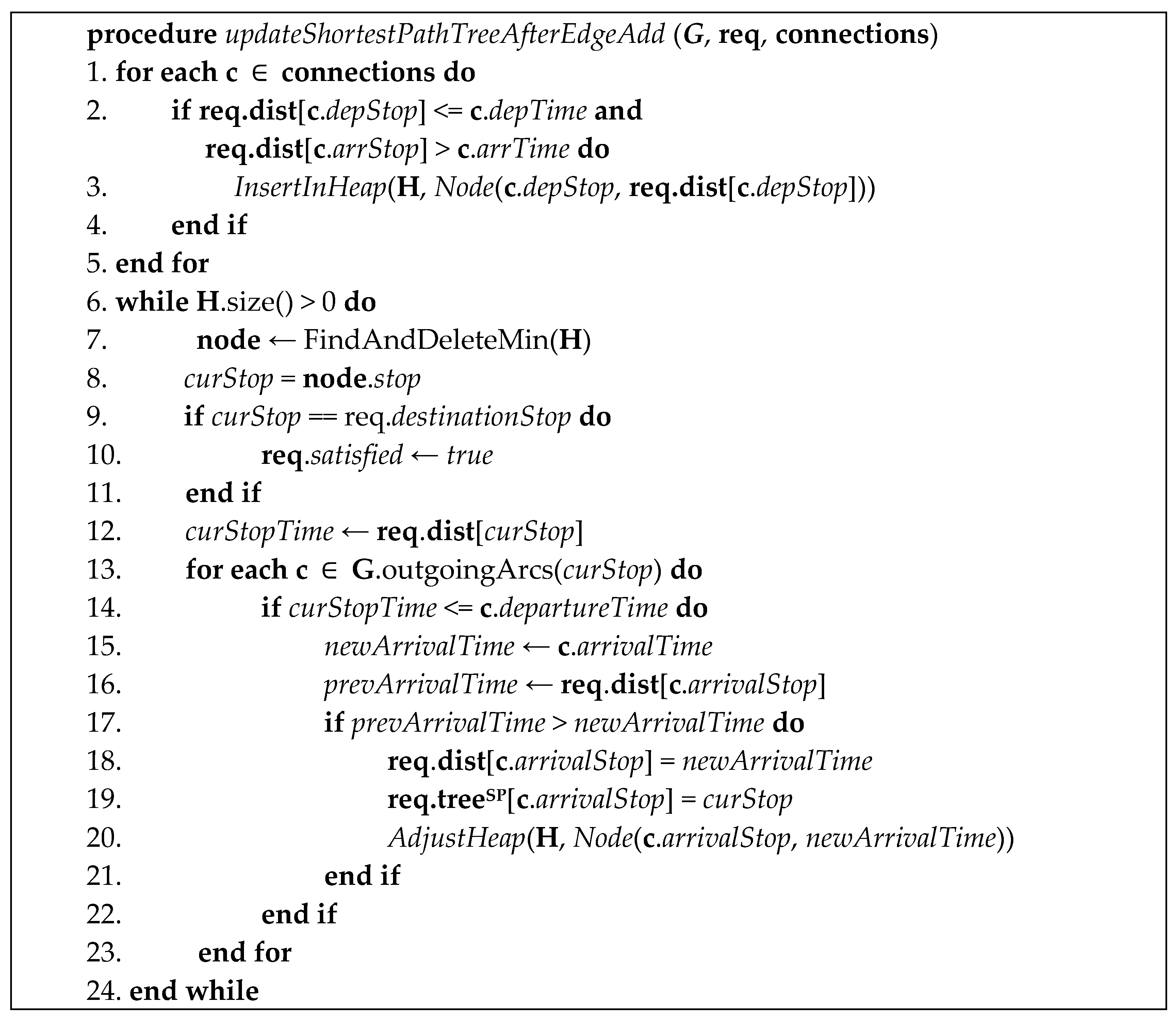
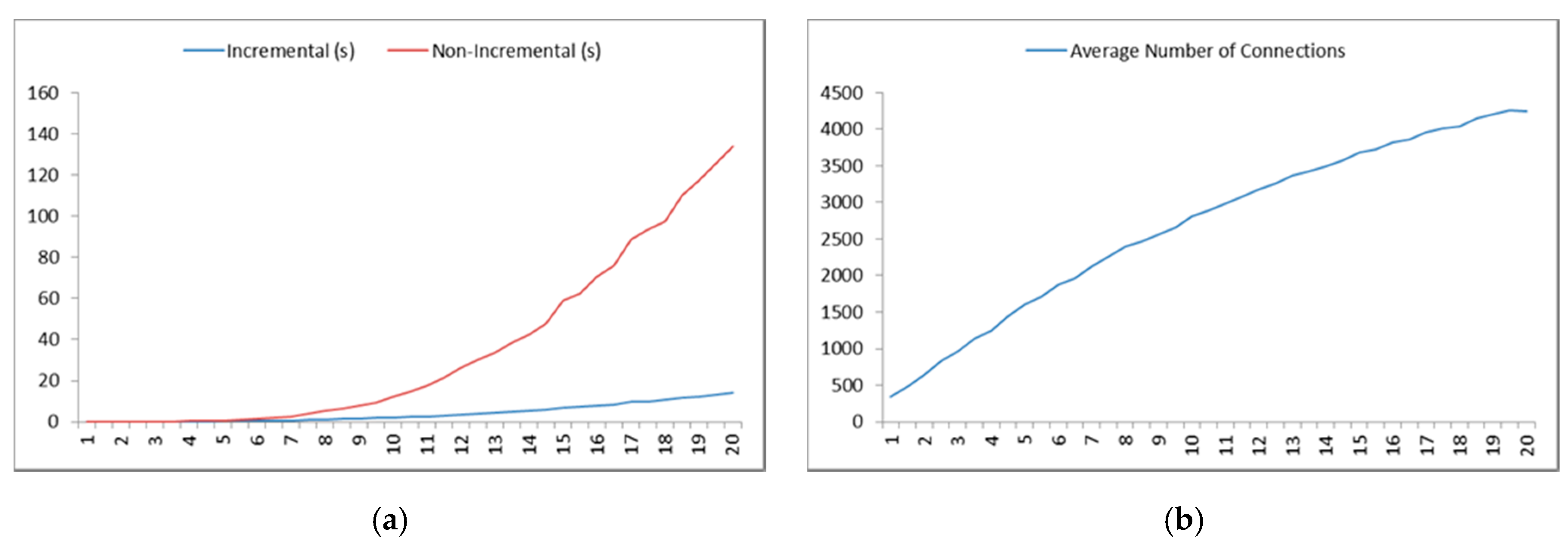
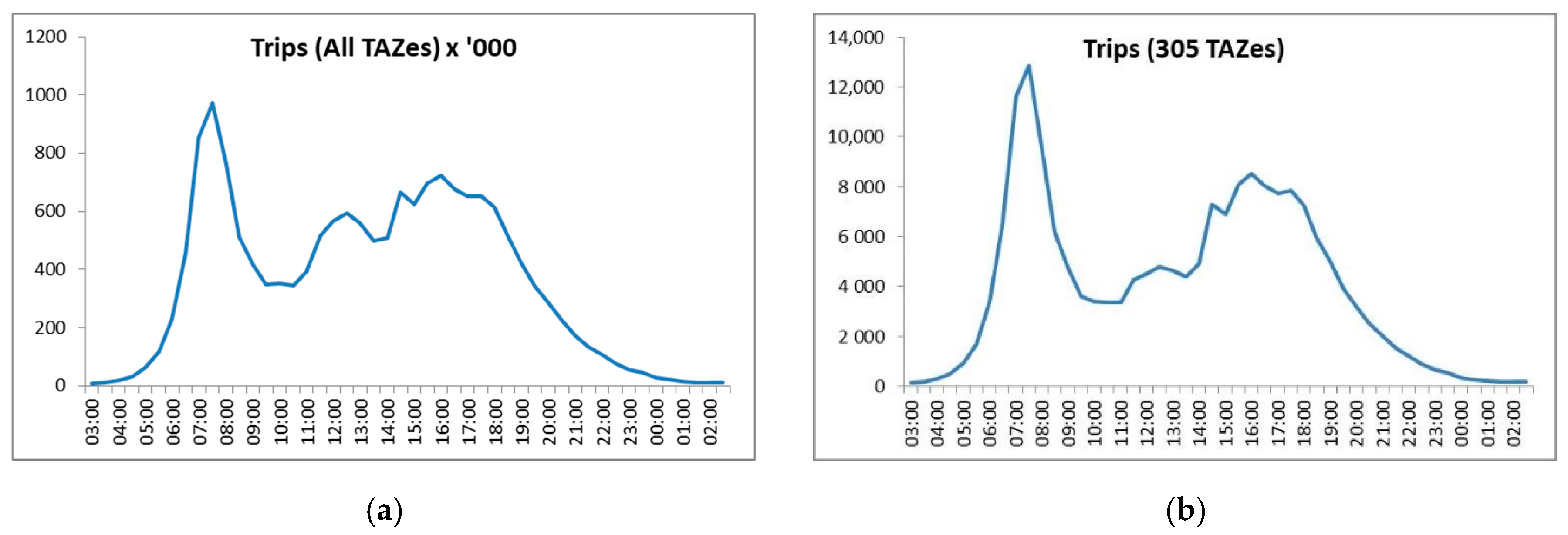
Table 1.
Matching rates for single-hop and multi-hop ridesharing.
| # Routes (# Hops) | Total Trips | # Offers | # Requests | # Matches | % Matches |
|---|---|---|---|---|---|
| Single-Hop | 190,142 | 95,048 | 95,093 | 28,231 | 30% |
| 1(1) | 190,142 | 95,166 | 94,975 | 28,306 | 30% |
| 1(2) | 190,142 | 95,028 | 95,113 | 49,720 | 52% |
| 1(3) | 190,142 | 95,005 | 95,136 | 63,614 | 67% |
| 2(1, 2) | 190,142 | 95,156 | 94,985 | 50,739 | 53% |
| 2(1, 3) | 190,142 | 95,162 | 94,979 | 64,426 | 68% |
| 2(2, 3) | 190,142 | 95,046 | 95,046 | 64,093 | 67% |
| 3(1, 2, 3) | 190,142 | 95,009 | 95,009 | 64,996 | 68% |
Table 2.
Number of hops in the shared rides.
| No. of Hops in Shared Rides | |||||||
|---|---|---|---|---|---|---|---|
| # Routes (# Hops) | Total Shared Rides | 1 Hop | 2 Hops | 3 Hops | 4 Hops | 5 Hops | |
| Single-Hop | # of rides | 28,231 | 28,231 | 0 | 0 | 0 | 0 |
| % age | 100 | 0 | 0 | 0 | 0 | ||
| 1(1) | # of rides | 28,306 | 28,305 | 1 | 0 | 0 | 0 |
| % age | 100 | 0 | 0 | 0 | 0 | ||
| 1(2) | # of rides | 49,720 | 33,731 | 15,619 | 371 | 1 | 0 |
| % age | 67.8 | 31.4 | 0.7 | 0 | 0 | ||
| 1(3) | # of rides | 63,614 | 33,353 | 26,982 | 3186 | 94 | 1 |
| % age | 52.4 | 42.4 | 5 | 0.1 | 0 | ||
| 2(1, 2) | # of rides | 50,739 | 37,890 | 12,559 | 289 | 1 | 0 |
| % age | 74.7 | 24.8 | 0.6 | 0 | 0 | ||
| 2(1, 3) | # of rides | 64,426 | 36,601 | 25,029 | 2718 | 78 | 1 |
| % age | 56.8 | 38.8 | 4.2 | 0.1 | 0 | ||
| 2(2, 3) | # of rides | 64,093 | 37,005 | 24,469 | 2558 | 61 | 1 |
| % age | 57.7 | 38.2 | 4 | 0.1 | 0 | ||
| 3(1, 2, 3) | # of rides | 64,996 | 38,267 | 24,260 | 2408 | 60 | 0 |
| % age | 58.9 | 37.3 | 3.7 | 0.1 | 0 | ||
Table 3.
System-wide total vehicle miles, with and without ridesharing.
| Without Ride Sharing | With Ride Sharing | ||||||
|---|---|---|---|---|---|---|---|
| # Routes (# Hops) | Total | Drivers | Riders | Total | Drivers | Riders | |
| Single-Hop | Vehicle Miles | 1,937,032 | 968,356 | 968,676 | 1,754,198 | 968,356 | 785,841 |
| % Change | −9.44 | ||||||
| 1(1) | Vehicle Miles | 1,937,032 | 969,024 | 968,008 | 1,753,451 | 969,024 | 784,427 |
| % Change | −9.5 | ||||||
| 1(2) | Vehicle Miles | 1,937,032 | 969,249 | 967,783 | 1,889,384 | 1,244,172 | 645,212 |
| % Change | −2.46 | ||||||
| 1(3) | Vehicle Miles | 1,937,032 | 968,253 | 968,779 | 2,171,785 | 1,646,400 | 525,385 |
| % Change | 12.12 | ||||||
| 2(1, 2) | Vehicle Miles | 1,937,032 | 969,233 | 967,799 | 1,701,850 | 1,065,845 | 636,005 |
| % Change | −12.14 | ||||||
| 2(1, 3) | Vehicle Miles | 1,937,032 | 969,382 | 967,650 | 1,862,026 | 1,348,964 | 513,062 |
| % Change | −3.87 | ||||||
| 2(2, 3) | Vehicle Miles | 1,937,032 | 968,811 | 968,221 | 1,915,395 | 1,396,055 | 519,340 |
| % Change | −1.12 | ||||||
| 3(1, 2, 3) | Vehicle Miles | 1,937,032 | 970,472 | 966,560 | 1,777,257 | 1,270,818 | 506,439 |
| % Change | −8.25 | ||||||
Table 4.
Driving and journey times with and without ridesharing.
| Without Ride Sharing | With Ride Sharing | ||||||
|---|---|---|---|---|---|---|---|
| # Routes (# Hops) | Total | Drivers | Riders | Total | Drivers | Riders | |
| Single-Hop | Driving time | 5,012,511 | 2,505,802 | 2,506,708 | 4,422,048 | 2,505,802 | 1,916,245 |
| % Change | −11.78 | 0 | −23.56 | ||||
| Journey time | 5,355,301 | 2,505,802 | 2,849,499 | ||||
| % Change | 6.84 | 0 | 13.67 | ||||
| 1(1) | Driving time | 5,012,511 | 2,508,076 | 2,504,434 | 4,420,003 | 2,508,076 | 1,911,927 |
| % Change | −11.82 | 0 | −23.66 | ||||
| Journey time | 5,356,673 | 2,508,076 | 2,848,597 | ||||
| % Change | 6.87 | 0 | 13.74 | ||||
| 1(2) | Driving time | 5,012,511 | 2,507,610 | 2,504,900 | 5,018,772 | 3,532,178 | 1,486,593 |
| % Change | 0.12 | 40.86 | −40.65 | ||||
| Journey time | 7,061,415 | 3,532,178 | 3,529,236 | ||||
| % Change | 40.88 | 40.86 | 40.89 | ||||
| 1(3) | Driving time | 5,012,511 | 2,505,690 | 2,506,820 | 5,978,315 | 4,824,037 | 1,154,278 |
| % Change | 19.27 | 92.52 | −53.95 | ||||
| Journey time | 9,041,034 | 4,824,037 | 4,216,996 | ||||
| % Change | 80.37 | 92.52 | 68.22 | ||||
| 2(1, 2) | Driving time | 5,012,511 | 2,508,778 | 2,503,732 | 4,368,025 | 2,909,390 | 1,458,635 |
| % Change | −12.86 | 15.97 | −41.74 | ||||
| Journey time | 6,272,000 | 2,909,390 | 3,362,610 | ||||
| % Change | 25.13 | 15.97 | 34.3 | ||||
| 2(1, 3) | Driving time | 5,012,511 | 2,508,695 | 2,503,815 | 4,995,438 | 3,872,414 | 1,123,023 |
| % Change | −0.34 | 54.36 | −55.15 | ||||
| Journey time | 7,893,168 | 3,872,414 | 4,020,754 | ||||
| % Change | 57.47 | 54.36 | 60.59 | ||||
| 2(2, 3) | Driving time | 5,012,511 | 2,507,030 | 2,505,480 | 5,183,796 | 4,044,579 | 1,139,216 |
| % Change | 3.42 | 61.33 | −54.53 | ||||
| Journey time | 8,038,910 | 4,04,4579 | 3,994,330 | ||||
| % Change | 60.38 | 61.33 | 59.42 | ||||
| 3(1, 2, 3) | Driving time | 5,012,511 | 2,509,950 | 2,502,560 | 4,725,407 | 3,617,905 | 1,107,502 |
| % Change | −5.73 | 44.14 | −55.75 | ||||
| Journey time | 7,522,365 | 3,617,905 | 3,904,460 | ||||
| % Change | 50.07 | 44.14 | 56.02 | ||||
Publisher’s Note: MDPI stays neutral with regard to jurisdictional claims in published maps and institutional affiliations. |
© 2020 by the authors. Licensee MDPI, Basel, Switzerland. This article is an open access article distributed under the terms and conditions of the Creative Commons Attribution (CC BY) license (http://creativecommons.org/licenses/by/4.0/).
Share and Cite
MDPI and ACS Style
Shah, I.; El Affendi, M.; Qureshi, B. SRide: An Online System for Multi-Hop Ridesharing. Sustainability 2020, 12, 9633. https://0-doi-org.brum.beds.ac.uk/10.3390/su12229633
AMA Style
Shah I, El Affendi M, Qureshi B. SRide: An Online System for Multi-Hop Ridesharing. Sustainability. 2020; 12(22):9633. https://0-doi-org.brum.beds.ac.uk/10.3390/su12229633
Chicago/Turabian StyleShah, Inayatullah, Mohammed El Affendi, and Basit Qureshi. 2020. "SRide: An Online System for Multi-Hop Ridesharing" Sustainability 12, no. 22: 9633. https://0-doi-org.brum.beds.ac.uk/10.3390/su12229633
Note that from the first issue of 2016, this journal uses article numbers instead of page numbers. See further details here.