Urban Development Modeling Using Integrated Fuzzy Systems, Ordered Weighted Averaging (OWA), and Geospatial Techniques

Abstract

This paper proposes a model to identify the changing of bare grounds into built-up or developed areas. The model is based on the fuzzy system and the Ordered Weighted Averaging (OWA) methods. The proposed model consists of four main sections, which include physical suitability, accessibility, the neighborhood effect, and a calculation of the overall suitability. In the first two parts, physical suitability and accessibility were obtained by defining fuzzy inference systems and applying the required map data associated with each section. However, in order to calculate the neighborhood effect, we used an enrichment factor method and a hybrid method consisting of the enrichment factor with the Few, Half, Most, and Majority quantifiers of the ordered weighted averaging (OWA) method. Finally, the three maps of physical suitability, accessibility, and the neighborhood effect were integrated by the fuzzy system method and the quantifiers of OWA to obtain the overall suitability maps. Then, the areas with high suitability were selected from the overall suitability map to be changed from bare ground into built-up areas. For this purpose, the proposed model was implemented and calibrated in the first period (2004–2010) and was evaluated by being applied to the second period (2010–2016). By comparing the estimated map of changes to the reference data and after the formation of the error matrix, it was determined that the OWA-Majority method has the best estimation compared to those of the other methods. Finally, the total accuracy and the Kappa coefficient for the OWA-Majority method in the second period were 98.98% and 98.98%, respectively, indicating this method’s high accuracy in predicting changes. In addition, the results were compared with those of other studies, which showed the effectiveness of the suggested method for urban development modeling.

1. Introduction

Nowadays, the rapid growth of urban populations in the world—especially in developing countries—causes a variety of problems in economic, environmental, social, and cultural spheres. The 2019 statistics suggest that there is a growth of 111,000 people in the population of Asia every day, and over a 25 year time period, from 1992 to 2016, an area of 144,000 km² of non-urban land became urban [1,2]. Increasing urban population growth and migration to cities has increased population density in cities. In such a situation, it is necessary for the city, as a base for urbanites, to provide indicators that might be called, at a glance, the standards of urban quality of life. The growth of urbanization and the tendency of individuals towards urban environments highlighted the concept of the quality of urban life more than ever. Therefore, the urban environment should have the capacity for urbanization [3]. Thus, the main question regarding the development of urban settlements and urban land use changes is whether it is possible to predict the conversion of non-urban land use into urban land use while the urban areas are quickly developing and changing. With this in mind, we tried to investigate the predictability of the development and the conversion of the bare grounds into developed lands in our attempt to answer this question, which is the main aim of this study. With the growth of urbanization, the concepts associated with sustainable development have emerged. In this regard, various studies have been carried out in different areas to determine the suitability of different sites [4,5,6].

According to the World Urbanization Prospect of the United Nations, 55% of the world population comprises urban population, while only 30% of the world’s population lived in cities in the 1950s. This percentage will reach 68% by 2050, and this is in spite of the fact that the entire urban area covers only 1% or 2% of the earth’s surface [7]. Therefore, this high population density and the general need to provide basic resources will result in an uneven utilization of resources [8].

Population growth and urban sprawl are not issues that could be easily controlled. Therefore, in recent years, the necessity of addressing this issue is felt in the evaluation and monitoring process of urban planning and urban development management [8]. Recently, there has been a significant increase in the use of Geospatial Information System (GIS) as an analytical and management tool for spatial data that can provide adequate support for decision making and planning of urban issues including urban development. In the past, the determination of land suitability, including spatial and descriptive comparisons, was carried out manually, whereas nowadays, these studies are simply conducted by the advanced GIS technology. Furthermore, thanks to the rapid development of GIS, land suitability analysis is used extensively for planning in many fields including agricultural activities [9], the determination of animal and plant habitats [10], landscape evaluation and planning [11], and regional planning and environmental impact assessment [12].

With this in mind, urban designers and environmentalists have attempted to achieve a comprehensive urban and environmental program by proposing solutions that can help to take decisive steps in optimally managing natural resources and properly using land. Two factors help them to achieve their goals more effectively; the first is to predict future land use status, and the second is to predict the outcomes of future strategies. Thus, urban development models could serve as a tool for designing macro urban management policies.

The spatial patterns of world urban development have been monitored and assessed using the advanced technologies of remote sensing and GIS techniques over the past few years [13,14]. Therefore, this has drawn the attention of researchers and engineers to the integration of mathematical and statistical methods into remote sensing and GIS data in order to model and map urban development [15]. Recently, a variety of approaches—including dynamic process-based methods, empirical statistical methods, stochastic and optimization methods, cellular automata (CA), and hybrid approaches—have been utilized to monitor urban development [16].

Dynamic process-based methods incorporate biophysical and socio-economic factors in order to simulate the spatial–temporal urban dynamics, and additional transitions of land-use changes are built based on simulated patterns [17]. Stochastic methods use historical trends of urban change to determine the possibilities of land-use changes based on several exogenous variables, whereas empirical statistical methods consider statistical methods such as multiple linear regression to analyze the effects of driving variables on urban development. Optimization methods are based on macro-economic factors using population-based optimization methods such as particle swarm optimization (PSO) and ant colony optimization (ACO), and on micro-economic factors using a linear programming approach. The cellular automatic method is regarded as a self-reproducing process that takes into account the neighborhood effect so as to incorporate the transition probabilities to further replicate the patterns of urban growth [18,19,20,21,22]. This approach is very similar to diffusion limited aggregation (DLA) and grid-based methods [23,24]. Hybrid methods are combinations of various modeling methods that simulate the complicated structure of urban dynamics. However, each modeling method has both advantages and limitations in addressing the effects of driving factors and disparate kinds of landscape structures [25].

In addition to these, other methods have been utilized to predict urban development and to assess urban spatial patterns, examples of which include the artificial neural networks [21,26], analytic hierarchy process (AHP) [27], SLEUTH model [28,29], spatial patterns analysis (SPA) [30,31], decision trees [21,32], Markov chains [33,34], Shannon’s entropy [35,36,37], fuzzy systems [20], principal component analysis (PCA) [36,38,39], and logistic regression [34]. Thus, the main contribution of this study is the designing of a method to predict the development of bare grounds into built-up areas using the fuzzy concepts and ordered weighted averaging (OWA) methods, which have not been applied in the literature, and to compare the results of these methods. For this purpose, the factors influencing urban change and development were identified and used in the modeling. Then, the proposed model was designed to take the input factors into account. In this study, the model, designed to evaluate the urban development of the Shiraz metropolis in Iran, was calibrated in the first time period (2004–2010) and then used for prediction in the second period (2010–2016).

2. Data and Study Area

2.1. Study Area

The study area is the Shiraz metropolis, the capital of Fars province in Iran. Shiraz is situated in the southwest of Iran. This city is one of the oldest cities in Iran, which has been a regional center of trade for well over a thousand years, and has temperate weather and a moderate climate. According to the latest census of the Statistical Center of Iran in 2016, this city had a population of 1,214,808, which increased to 1,405,073 in 2010, and 1,712,745 in 2016. Its built-up region is home to 1,565,572 residents. Shiraz was used as the case study because it is undergoing unfavorable ecological loss resulting from relatively uncontrolled and fast urban growth. During the studied period, a large area of the previously bare grounds changed into developed areas. Furthermore, this increased population has given rise to development projects that have resulted in great energy expenditures, pollution, and miserable living conditions. Therefore, reasonable land-use modeling and planning are necessarily needed to reduce the adverse ecological consequences and to keep up with the speed of urban growth. The location of Shiraz in the Fars province is shown in Figure 1.

2.2. Data

The proposed model attempts to take important parameters and land uses (which can be modeled with their available data) as inputs of the model. The required data for both time periods of 2004–2010 and 2010–2016 are as follows:

(1) Digital Elevation Model (DEM) and Digital Surface Model (DSM) with a resolution of 50 m for baseline years (2004 for the first time period and 2010 for the second time period). The DEM map used in this study is related to the ASTER Global Digital Elevation Model, in which its pixel size is resampled to 50 meters, similarly to the pixels used in urban maps.

(2) Main and sub-road vector layers in baseline years.

(3) Land-use map of the city in the baseline years (2004 and 2010) with a resolution of 50 m, including minimum administrative, industrial, sports, residential, bare, and therapeutic uses.

(4) Land-use maps of the city (2016) with a resolution of 50 m. These maps are only used to evaluate the results of the model and have no direct application in forecasting and modeling. Urban land-use maps, which were prepared by land surveying and aerial photo interpretation, were obtained from the Department of Roads and Urban Development of Shiraz.

3. Fuzzy Inference Systems

Fuzzy logic was first proposed by [40] to model continuous processes and as a tool to develop from the theory of binary sets into continuous sets. In modeling each target or criterion in a fuzzy method, each set or parameter has a membership function. Membership functions get the parameter values and determine the membership degree of any value of the parameter attributed to the specified target. It should be noted that fuzzy sets can have multiple membership functions for a variable. Membership functions can be triangular, trapezoidal, Gaussian, and so on. The selection of the membership function type and its parameters depends on the type and nature of the problem. In order to design fuzzy systems, an expert is needed to use their fuzzy knowledge in designing fuzzy systems in such a way that they can behave similarly to an expert. Rule-based systems are another type of expert system that can solve many problems by applying human knowledge as “if–then” rules and modeling them in the best way possible. Fuzzy rule-based systems are created using fuzzy logic in rule-based systems. One of the advantages of fuzzy rule-based systems compared to the classic rule-based systems is the possibility of using fuzzy sets that have uncertainty, as well as greater flexibility and stability in the inference method using fuzzy logic [3]. A fuzzy rule-based system consists of the following parts:

A) Fuzzification: In this section, a non-fuzzy input is entered and mapped as a fuzzy set according to the defined fuzzy functions.

B) Database: This section contains the required information about the input variables as well as the relations governing them. It consists of the database and the rule base. The database provides the necessary definitions for membership functions associated with linguistic variables and membership functions. The rule base contains a set of if–then conditional rules, and the output of the system is determined using this set of rules.

C) Inference system: In this section, an inference method is applied, and a fuzzy output is obtained based on the input of the system, which is made fuzzy by Fuzzification, as well as the information and rules of the database. In this study, the Mamdani method (minimum–maximum) is used according to Equation (1).

$$y_i=Ma{x}_{k=1,2,\dots ,n}\{{\mathrm{Min}}_k[{\mu }_d(i,j),{\mu }_h(i,j)]\}$$

(1)

In the above Equation, μ is the membership function value for the input variables, and k is the total number of fuzzy rules.

D) Defuzzification: In this phase, the output fuzzy set of the inference system is mapped to a definite output. There have been a variety of methods proposed for Defuzzification, among which the Center of Gravity (CoG) method is the most common. This method can be defined as in Equation (2).

$$y=\frac{{\displaystyle \sum _{i=1}^N{y}_i}{\mu }_{out}(y_i)}{{\displaystyle \sum _{i=1}^N{\mu }_{out}(y_i)}},$$

(2)

where N indicates the number of points considered on the output fuzzy function with the membership function of μ_out, y_i represents the value of each point in the horizontal axis of the output membership function, and y denotes the defuzzied value.

4. Proposed Method

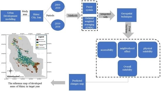
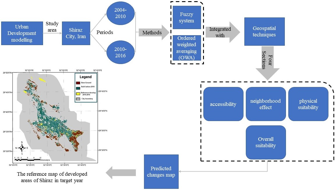
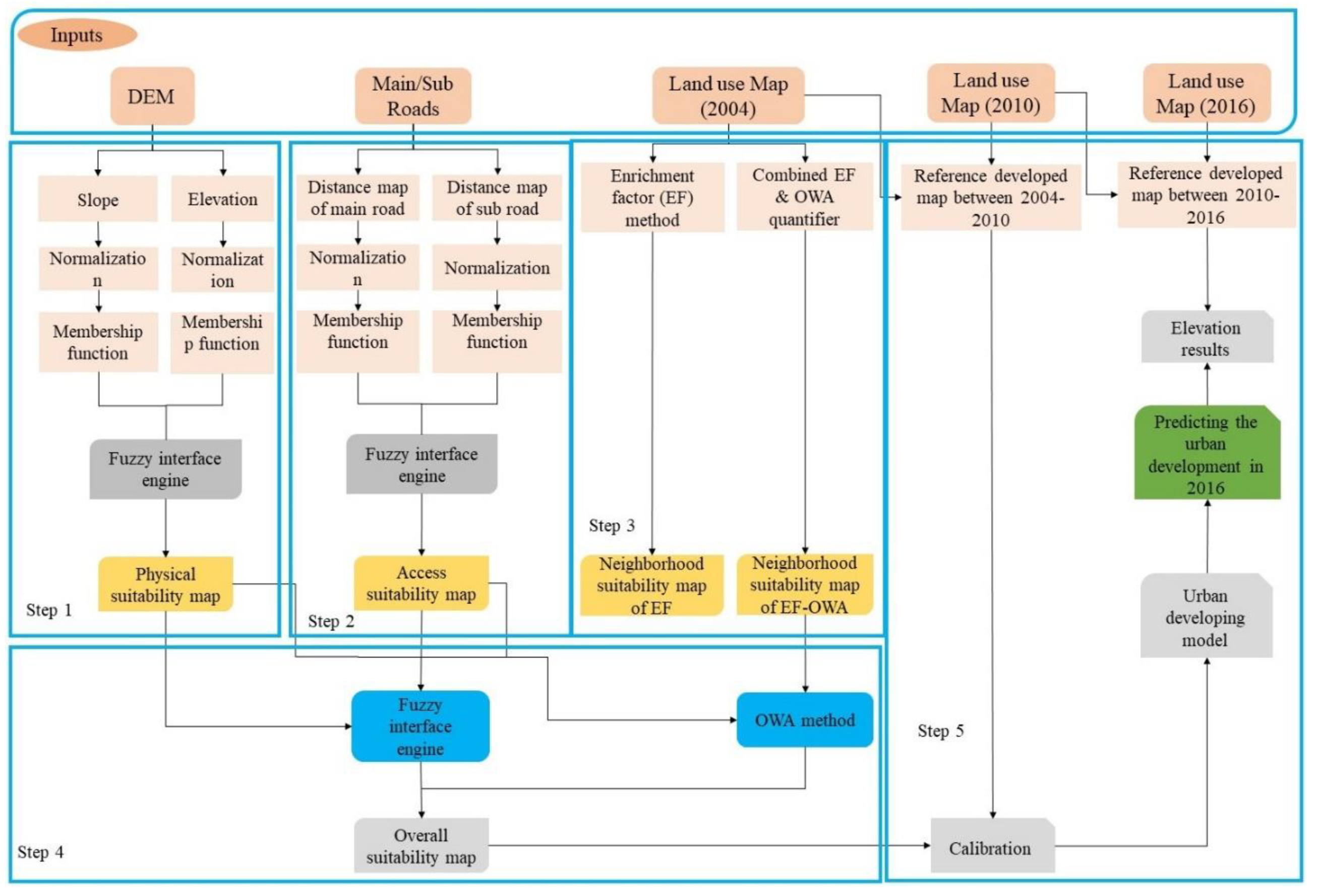
The overall structure of the model proposed in this study is based on fuzzy logic and OWA methods (Figure 2). The proposed model can be implemented through the following five main stages.

The first stage is to determine physical suitability. At this stage, the elevation and slope layers of Shiraz are used. The second stage is to calculate the accessibility of the main and sub roads. At this stage, using the main- and sub-road layers and by defining the fuzzy system, the accessibility of each point to the transportation network is calculated in order to produce the accessibility suitability map. The third stage is to calculate the neighborhood effect. The enrichment factor and OWA (EF-OWA) methods are employed for calculation. The effect of residential, industrial, recreational, administrative, and therapeutic uses on each bare pixel is calculated in order to produce a map of the neighborhood effect or suitability. At this stage, one output is produced for the neighborhood effect map using the enrichment factor method, and four outputs of the neighborhood effect map are generated by a combination of the OWA quantifiers (EF-OWA-Quantifiers) and the enrichment factor.

The fourth stage is to calculate the overall suitability map (combining the results of the previous three stages). At this stage, physical suitability, accessibility, and neighborhood effect maps that were obtained in the first three stages are taken as inputs. Since five neighborhood effect maps are produced in the previous step, five overall suitability maps are produced at this stage. In generating overall suitability maps, the physical suitability and accessibility maps are fixed. Furthermore, in the method where the neighborhood effect is produced by the enrichment factor method, its overall suitability map is obtained by the fuzzy method. In the other four methods in which the neighborhood map is generated through a combination of the enrichment factor and OWA quantifiers methods, the overall suitability maps are obtained using the OWA method.

In the fifth stage, the urban development model is calibrated for a six-year time period, and the developed areas map forecasted for 2016 is evaluated using a reference map of the developed areas of the same six-year time period.

4.1. Determination of Physical Suitability

In this study, slope and elevation factors are regarded as two factors involved in urban growth. Renzhi Liu considers a slope of 0%–2% to be ideal for urbanism, while it is suitable up to 5% and not suitable over 10% [41]. In this study, after normalizing the maps of slope and elevation in a 0–1 range, the input and output membership functions of physical suitability are taken into account. Then, the fuzzy rules are defined according to

Table 1. Fuzzy rules applied in the fuzzy inference engine to determine physical suitability.

		Elevation
		Low	Moderate	High
Slope	Low	Very Good	Good	Moderate
	Moderate	Moderate	Bad	Very Bad
	High	Bad	Very Bad	Very Bad

in order to connect the input and output functions. After defining the membership functions and fuzzy rules, the physical suitability map of the study area is produced using the Mamdani fuzzy inference engine.

4.2. Determination of Accessibility Suitability

In this study, given the data available, access to main and sub-roads is considered a factor affecting urban growth. At this stage, as in the stage of determining physical suitability, the distance map of the main and sub-roads is generated and normalized to evaluate accessibility. Then, the membership function of distance is used for fuzzification. It should be noted that in this study, the output membership function for physical suitability, accessibility suitability, and neighborhood effect is taken into account. Moreover, the fuzzy rules in

Table 2. Fuzzy rules applied in the fuzzy inference engine to determine accessibility suitability.

		Distance from Sub-Roads
		Low	Moderate	High
Distance from Main Roads	Low	Very Good	Good	Moderate
	Moderate	Good	Moderate	Bad
	High	Moderate	Bad	Very Bad

are used to determine accessibility suitability.

4.3. Determination of Neighborhood Suitability

In this study, the neighborhood effect was calculated by the enrichment factor and EF-OWA-Quantifiers methods, as described below. It is worth noting that the neighborhood effect is calculated only for the bare pixels, since the purpose in both methods is to forecast the changing of bare ground into built-up areas.

4.3.1. Enrichment Factor

The neighborhood effect on each pixel is calculated from the overall neighborhood effect of the pixels adjacent to the radius of influence and according to their use and distance. The neighborhood effect determines which cells have more potential to change. If a radial neighborhood with a radius of eight pixels is considered, it is 172 pixels. In the enrichment factor method, the effect of adsorption or excretion of each of the adjacent 172 pixels is illustrated on the central pixel. Typically, the cells farther from the central cell have less effect on it. In order to calculate the neighborhood effect, the enrichment factor diagram should first be extracted. This diagram illustrates the effects of different uses on each other at different distances; for example, industrial use can have an excretion effect on residential uses, or residential uses can have an adsorption effect on bare uses. In other words, there are more residential pixels around bare pixels. The following steps should be taken one by one in order to extract the enrichment factor diagram:

Step 1: First, the total density of each residential, administrative, industrial, therapeutic, sports, recreational, and bare use in the study area is calculated. For example, the total density of a residential use, according to Equation (3), is calculated by dividing the total number of residential pixels (N_Residential) into the total number of pixels (N) [42].

$$T{D}_{Res}=\frac{N_{Residential}}{N}$$

(3)

Step 2: The local densities of each use are computed at distances of one to eight pixels. For example, the local density of residential use at the distance d = 1 is calculated through Equation (4) [42]. In this Equation, ($N_{Residential}^1$) is the number of residential uses at d = 1 and N¹ is the total number of uses in this distance.

$$L{D}_{Residential}^1=\frac{N_{Residential}^1}{N^1}$$

(4)

Equation (5) is used to specify the distance of each pixel from the central pixel.

$$d=\sqrt{d{x}^2+d{y}^2}$$

(5)

Step 3: The spatial index of the enrichment factor at the distance d for the use k is calculated according to Equation (6) by dividing local density by total density [42].

$$F_k^d=\frac{L{D}_k^d}{T{D}_k}$$

(6)

A spatial index matrix is formed by calculating the spatial index of the enrichment factor ($F_k^d$) for each use. This matrix has rows based on the number of pixels in the land use map, and its columns represent the spatial index of the enrichment factor at different distances.

Step 4: A graph is depicted as a transfer function or neighborhood effect by using a spatial index matrix for each use. For this purpose, in each use and at each distance, the values of the enrichment factor are averaged so that the average vector of the enrichment factor is obtained for each use, with the rows indicating the average values of the enrichment factor at different distances. Finally, the enrichment factor graph for each use is obtained by applying the logarithm to its average vector of the enrichment factor.

Step 5: Finally, in order to calculate the final neighborhood effect of each pixel with bare use at different distances (d), it is necessary to obtain the number of uses present in the neighborhood. The impact of different uses (W_d-k) is extracted from the enrichment factor diagram; the neighborhood effect on each point, in accordance with Equation (7), is calculated from the sum of the neighborhood effects of all adjacent pixels with different distances and uses.

$$NE={\displaystyle \sum _k{\displaystyle \sum _d{W}_{d,k}}}$$

(7)

Since the neighborhood suitability map can have negative values due to the excretion effects of some uses (negative values), the neighborhood suitability map is normalized between zero and one.

4.3.2. Hybrid Method of the Enrichment Factor and OWA

Multi-criteria evaluation methods in GIS typically include a series of criteria to evaluate various options, and each option is allocated some weight according to those criteria. The problem of determining the neighborhood effect that different uses have on pixels can also be regarded as a multi-criteria problem. Therefore, multi-criteria decision-making techniques such as OWA can be used for calculation. In order to obtain the effect of different uses on the central pixel in the enrichment factor method, the effects of all uses were aggregated cumulatively. However, if the effect of each use is calculated individually and regarded as a criterion, the effects of various uses can be considered a multi-criteria problem, and their values can be combined to obtain a single number using different OWA quantifiers.

OWA quantifiers use standard and ordered weights. The standard weights indicate the relative importance of each evaluation criterion (layers and maps), whereas ordered weights are allocated based on the importance of the cells of layers and the maps. OWA quantifiers create different scenarios in terms of optimism or rigor and produce different weights. The quantifiers used at this stage are the three quantifiers Few, Half, and Most, as well as the majority-OWA method, which in total produce four outputs, forming the neighborhood effect map. The quantifiers used in this study will be described later on. Then, the production of the neighborhood effect map by these quantifiers is described.

Few quantifier: This is an optimistic quantifier [43]. In optimistic quantifiers, weights are defined in such a way that even if one or a few criteria have a suitable state for the options, the final value of the option is large [44].

Half quantifier: This is a moderate quantifier in terms of optimistic or rigorous approaches [43]. All components of the weight vector generated by this quantifier are approximately equal, and the effects of all uses are considered approximately equal in value and weight [44]. Therefore, the results obtained by this method are expected to be approximately the same as the results of the enrichment factor method.

Most quantifier: This quantifier has a rigorous approach [43]. In this quantifier, weights are defined in such a way that the only options that have a high value in the final evaluation are those for which all criteria are appropriate [45].

Majority quantifier: This quantifier has a different function compared to those of the other quantifiers. The way the weight vector is defined is regarded as the most important difference between this method and the others because the optimistic or rigorous concept is not taken into account in this method, and the concept of the majority is what matters; the weights are defined in such a way that the final assessment of the option is close to the opinion of the majority of the criteria. In this method, the criteria with closer values are weighed higher in order to provide the opinion of the majority [43].

In the following, the creation of the neighborhood effect map by EF-OWA-Quantifiers is described in three steps.

Step 1: First, using the enrichment factor method and Equations (4)–(6), the effect of each use is calculated separately for the desired pixel. The effect of each use is obtained from the total effect of that use on the desired pixel at different distances. The collection of effects creates a vector for each pixel, and the vectors are then arranged in ascending to descending order.

Step 2: For each of the Few, Half, and Most quantifiers, the weight vector $\overrightarrow{W}$ is obtained through Equations (8) and (9).

$$Q(P)=P^{\alpha }$$

(8)

$$\overrightarrow{W}=Q(\frac{i}{n})-Q(\frac{i-1}{n})\mathrm{where}i=1,\dots ,n,$$

(9)

where n represents the number of criteria, and $\alpha$ indicates a constant parameter taken to be 0.1, 1, and 10 for the quantifiers Few, Half, and Most, respectively [46]. The weight vector in the Majority quantifier is calculated in a different way. In the Majority quantifier, what matters when calculating the weight of each criterion is the sum of distances or the similarity of that criterion to the other criteria. In other words, a weight assigned to that criteria is proportionate to the reverse of the total distances of each criterion from the other criteria. For this purpose, the weight vector in the Majority-OWA method is determined according to Equations (10) to (12) [45]:

$${\delta }_i={\displaystyle \sum _{j=1}^{n}Dist(a_i,a_j)}\mathrm{Where}Dist(a_i,a_j)=\{\begin{array}{c}1\mathrm{if}\left|a_i-a_j\right|<x\hfill \\ 0\mathrm{otherwise}\hfill \end{array}$$

(10)

$$W_i=\frac{1}{{\displaystyle \sum _{i=1}^n{\delta }_i}}\mathrm{Where}{W}_i\in [0,1]\&{\displaystyle \sum _{i=1}^n{W}_i}=1$$

(11)

$$\overrightarrow{W}=(W_1,W_2,\dots ,W_n),$$

(12)

where the value of x is determined according to the problem conditions and the expert opinion, but experience indicated that using the standard deviation of the set of the effects of different uses provides appropriate results. In this study, instead of x, the standard deviation of the set of effects of different uses is applied.

Step 3: If the effects of uses sorted from ascending to descending and the weight vector of the j^th pixel are indicated with ($\overrightarrow{A_j}$) and ($\overrightarrow{W_j}$), respectively, then the neighborhood effect of the j^th pixel is obtained according to Equation (13) by a dot product of the vectors ($\overrightarrow{A_j}$) and ($\overrightarrow{W_j}$).

$$N{E}_j=\overrightarrow{W_j}.\overrightarrow{A_j}$$

(13)

Repeating the above steps for all pixels provides the neighborhood effect map in the EF-OWA-Quantifiers method. Since the neighborhood suitability map can also have negative values due to the excretion effects of some uses (negative values), the neighborhood map is normalized between zero and one.

4.4. Determination of Overall Suitability

After the creation of physical suitability, accessibility suitability, and neighborhood effect maps, these three maps are integrated in order to calculate the development potential of the bare pixels. In this study, in order to integrate the three aforementioned maps and to determine the final output, the two different methods of the fuzzy inference system and OWA quantifiers are used, producing a total of five outputs.

4.4.1. Fuzzy Inference System

In this method, the three maps of physical suitability, accessibility suitability, and neighborhood effect are integrated using a fuzzy inference system. In this study, in order to calculate the overall weight suitability or the impact of all the three maps, the physical suitability, accessibility suitability, and neighborhood effect are considered the same, and their input membership function is regarded as the membership function of the elevation parameter for fuzzification. In this study, the output membership function for the overall suitability is defined as the output membership function of physical suitability. After the input and output functions of the overall suitability are identified, it is necessary to define fuzzy rules to calculate the overall suitability. Some of these rules are presented in

Table 3. Some of the fuzzy rules applied in the fuzzy inference engine to determine overall suitability.

Physical Suitability	Accessibility Suitability	Neighborhood Effect	Overall Suitability
High	High	High	Very Good
Moderate	High	High	Good
High	High	Moderate	Good
High	Moderate	Low	Moderate
High	Low	Low	Bad
Moderate	Moderate	Moderate	Moderate
Moderate	High	Moderate	Good
Moderate	Low	Low	Very Bad
Low	Moderate	Moderate	Bad
Low	Low	Low	Very Bad

.

After determining the input and output membership functions and defining transfer rules, the Mamdani fuzzy inference engine method is used to integrate the input maps and generate the overall suitability. The overall suitability maps indicate the adequacy points for the development of bare ground uses into built-up areas.

4.4.2. OWA Quantifiers

In this method, physical suitability, accessibility suitability, and neighborhood effect maps are each integrated as criteria using the quantifiers Most, Half, Few, and OWA. For this purpose, using Equations (8) to (12), the weight vector is produced for each of the Most, Half, Few, and Majority quantifiers, the difference being that the number of criteria (n) in this integration is three and, instead of the vector of the effects of uses, we use the vector of suitability values with three entries. For this purpose, if the suitability values—ordered from ascending to descending—and the weight vector for the j^th pixel are respectively illustrated by ($\overrightarrow{B_j}$) and ($\overrightarrow{W_j}$), then the overall suitability of the j^th pixel, in accordance with Equation (14), is obtained by dot product of the ($\overrightarrow{B_j}$) and ($\overrightarrow{W_j}$) vectors.

$$O{S}_j=\overrightarrow{W_j}.\overrightarrow{B_j}$$

(14)

Therefore, four suitability maps are generated using OWA quantifiers.

4.5. Calibration of the Urban Development Model

At this stage, the urban development model is calibrated for a six-year period. In accordance with Equation (15), the developed areas are estimated for 2010 by putting thresholds on each of the overall suitability maps obtained in the period 2004–2010.

$$D{A}_m=O{S}_m>T{h}_1,$$

(15)

where m is the index of the method used to generate the overall suitability with values ranging from 1 to 5.

Therefore, five maps of the developed areas (four maps with a threshold on the overall suitability obtained by the OWA quantifiers and one map with a threshold on the overall suitability obtained by the fuzzy inference system) are generated, representing the areas likely to be developed, and are then evaluated and compared to the reference map of the developed areas in 2010. At this stage, putting thresholds on each of the overall suitability maps is performed in such a way that they are most closely matched to the reference map of the developed areas in the first time period, and the calibrated thresholds are obtained for each of the map integration methods. For this purpose, the Th₁ threshold value is changed with steady steps, and the precision or matching values between the estimated map and the reference map of the developed areas are obtained for each Th₁ threshold value; then, the best threshold is extracted for each of the five methods. Then, the thresholds obtained in the calibration process are applied to the overall suitability maps for the second time period (2010–2016). The purpose is to estimate the map of developed areas in 2016; then, this map is compared with the reference map of the developed areas in 2016 in order to obtain the evaluation results of the proposed model. In order to evaluate the proposed model, some indexes are used. These are described in the next section.

4.6. Result Evaluation Method

An important method of model evaluation is to examine the results of the proposed model and compare their conformity with reality. In this study, the error matrix is used to evaluate the accuracy of the proposed model [47]. In this evaluation, the reference map of the developed areas is compared with the estimated one. The general structure of the error matrix [48] in a classified image with N pixels used in this study is similar to

Table 4. General structure of the error matrix.

	Modeled
Reference	Classes	Developed	Bare	Row Marginal
	Developed	TP	FN	RM1
	Bare	FP	TN	RM2
	Column Marginal	CM1	CM2	N

.

In the above matrix, True Positive (TP) is the total number of pixels that are present in both modeled and real developed statuses. False Positive (FP) represents the number of pixels that are bare in reality and developed in the modeled map. False Negative (FN) indicates the number of pixels that are developed in reality, but the model does not consider any development for them by mistake. Moreover, True Negative (TN) denotes the number of pixels that have a bare use in both the reference and modeled maps [49].

One of the metrics derived from the error matrix to calculate accuracy is the overall accuracy (OA) index, which is calculated, as shown in Equation (15), by dividing the sum of the main diameters by the total number of pixels. Similarly, according to Equations (16) to (19), the Kappa coefficient, user’s accuracy (UA), and producer’s accuracy (PA) are calculated based on the following Equations [50].

$$OA=\frac{TP+TN}{N}$$

(16)

$$P_e=\frac{C{M}_1\times R{M}_1+C{M}_2\times R{M}_2}{N^2}$$

(17)

$$Kappa=\frac{OA-P_e}{1-P_e}$$

(18)

$$P{A}_{c1}=\frac{TP}{R{M}_1}\&P{A}_{c2}=\frac{TN}{R{M}_2}$$

(19)

$$U{A}_{c1}=\frac{TP}{C{M}_1}\&U{A}_{c2}=\frac{TN}{C{M}_2}$$

(20)

5. Results and Discussion

In this section, some suggestions are proposed and discussed in each part.

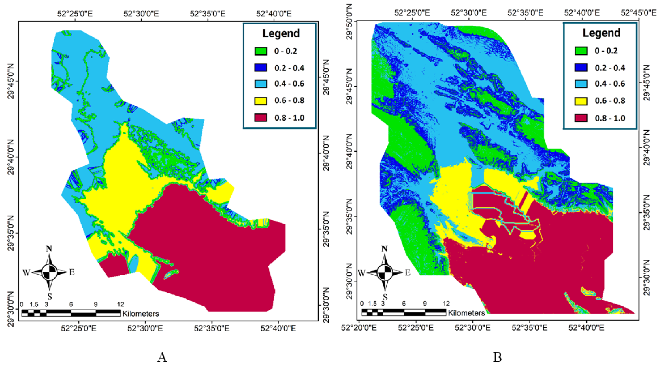
5.1. Physical Suitability

In this study, ArcMap 10.5 was used to generate slope maps from a digital terrain model (elevation map). In order to use the slope and elevation maps, based on the proposed method, it is necessary to normalize the elevation and slope information layers to values between zero and one.

After normalization, the maps were fuzzified using the input membership functions, and the physical suitability maps were obtained for both the first and second time periods by using the rule bases in Table 1 in a Mamdani fuzzy inference system. It is worth noting that all operations associated with the fuzzy inference system were performed in Matlab 2015. As shown in Figure 3, most of the study area has a moderate to high physical suitability (0.5–1).

5.2. Accessibility Suitability

At this stage, the distance maps of the main and sub-roads were generated in ArcMap 10.5. After the distance maps were normalized into values between zero and one, the input membership function was used to fuzzify the maps. In the Mamdani fuzzy inference system and based on the fuzzy rules in Table 2 and the output membership function, the distance maps were integrated in order to obtain an accessibility suitability map for the study area, the results of which are shown in Figure 4. As shown in Figure 4, a large part of the study area has high accessibility suitability.

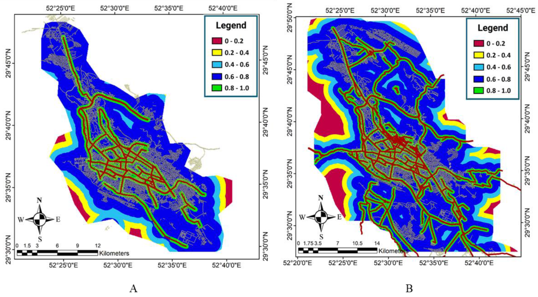
5.3. Neighborhood Effect

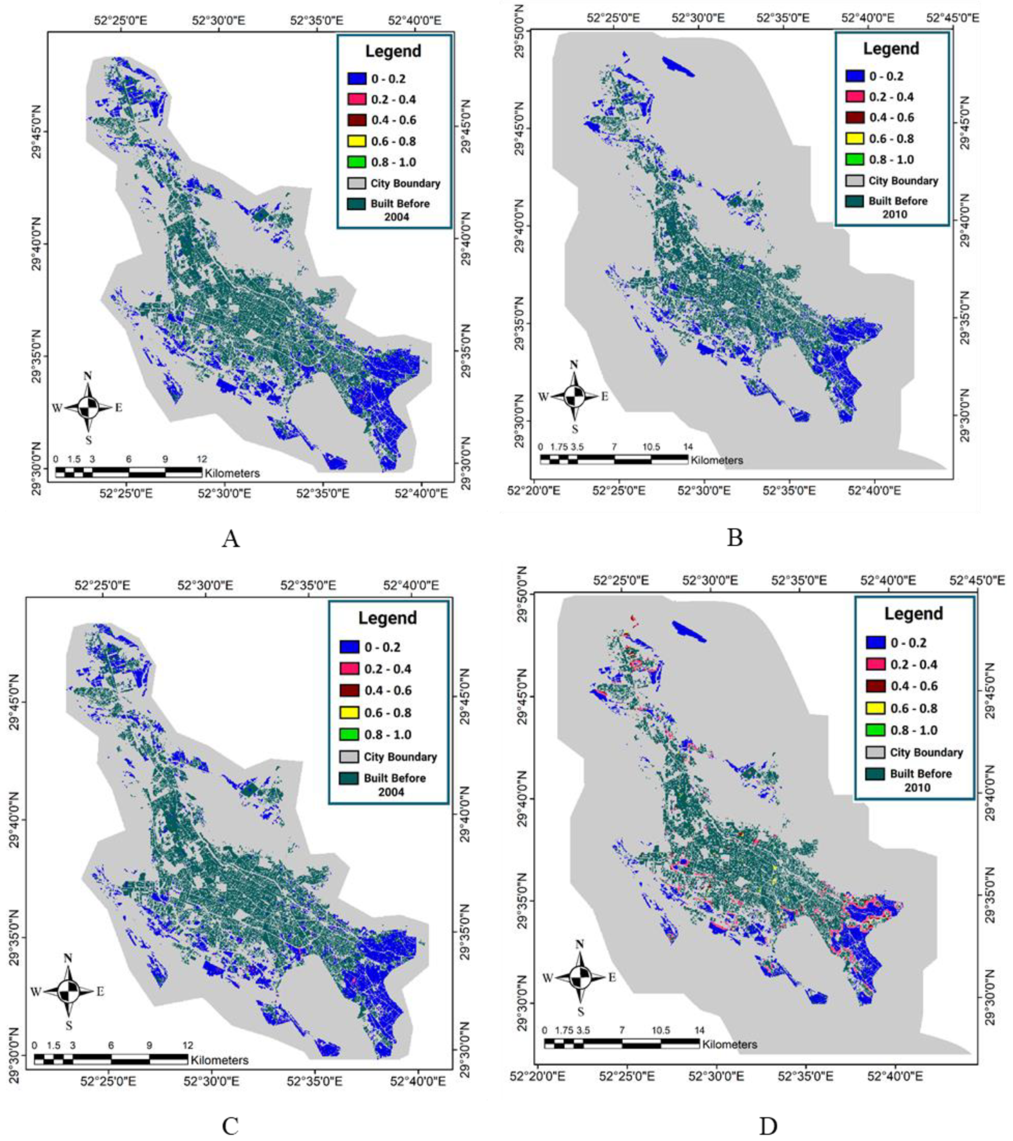
In order to calculate the neighborhood effect in this study, we used the land-use maps of Shiraz in the baseline years 2004 and 2010, with administrative, industrial, sports, residential, and therapeutic uses. The aim of this was to calculate the effect of the other pixels’ uses on the pixels that have bare ground use. Thus, it was possible to determine the bare pixels that were in a better condition to change into the urban state in terms of their neighboring pixels. The neighborhood space was taken to be a circle with the desired cell in the center and with a radius of eight pixels (400 meters). Thus, the neighborhood included 172 pixels; this is the distance at which pixels are affected by the central pixel. The neighborhood effect was calculated for all bare pixels using both the enrichment factor and EF-OWA-Quantifiers methods. As described in the proposed method, in the enrichment factor method, it is necessary to extract the enrichment factor diagrams of the effect of different uses on bare ground uses.

After extracting the enrichment factor diagram, the effect of different uses (W_d,k) was extracted from the enrichment factor diagram, and the neighborhood effect map (NE) was obtained with the total W_d,k for all uses and distances, as displayed for both time periods in Figure 5. Using the neighborhood effect map obtained by the enrichment factor (EF) method, it is observable that the effect of neighborhoods on the boundary between bare and residential lands is higher than on other points.

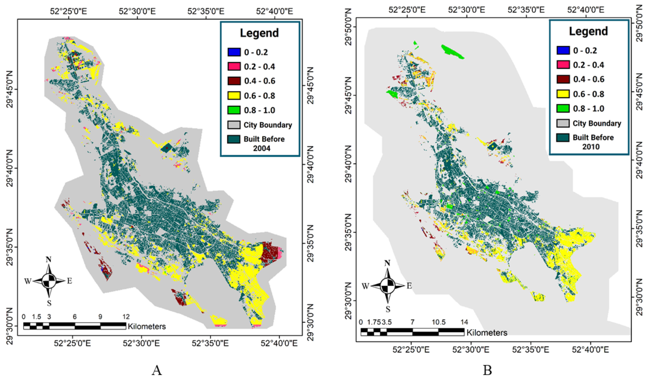
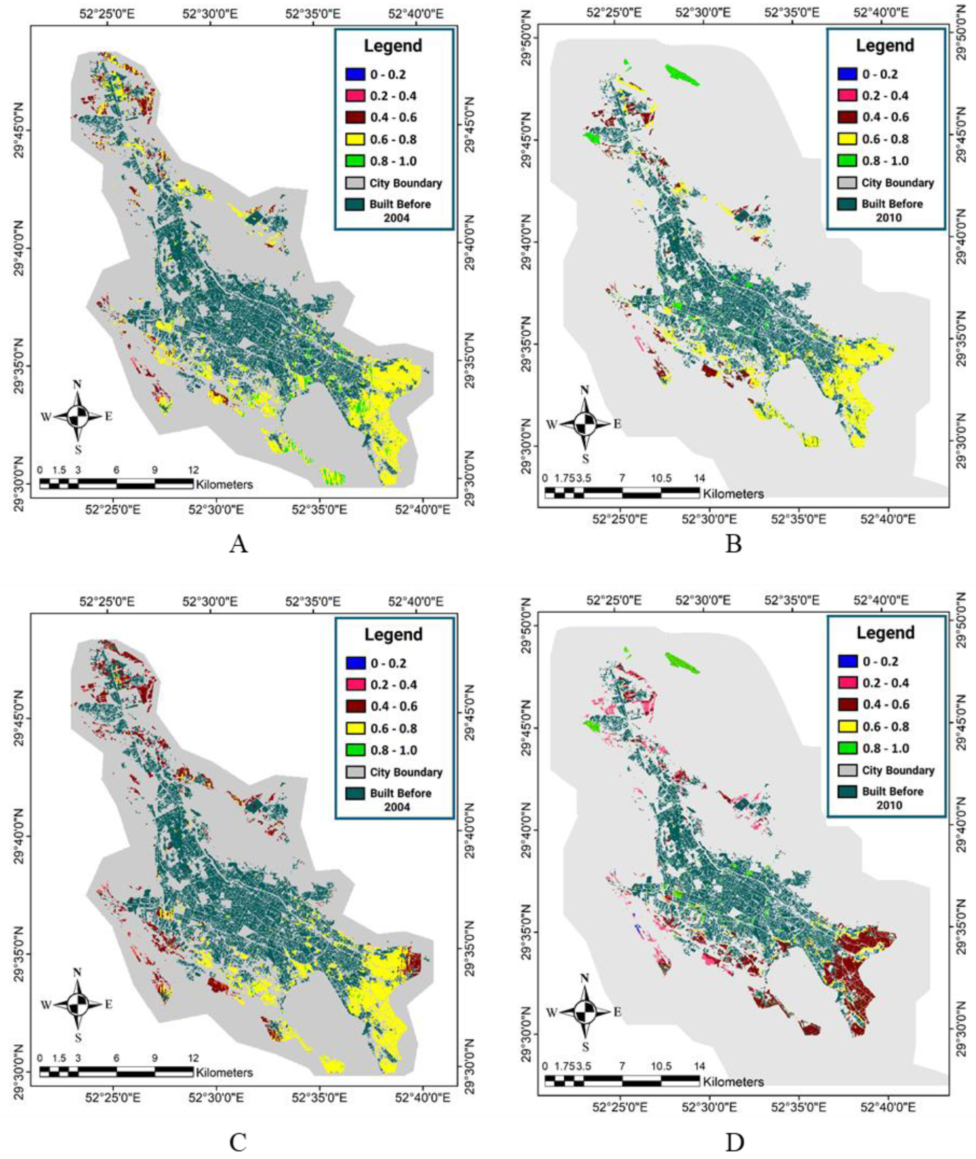
In the EF-OWA-Quantifiers method, the weight vector ($\overrightarrow{W}$) is calculated for each of the Few, Half, and Most quantifiers through Equations (8) and (9), and for the Majority quantifier through Equations (10) to (12). It is worth noting that the values of the weight vectors for the three quantifiers (Few, Half, and Most) are constant with the six criteria presented below. However, the weight vector values vary for the Majority quantifier, since it is dependent on the vector of land-use effects in each point of the study area.

W_Few = (0.8360, 0.0600, 0.0371, 0.0272, 0.217, 0.0181)

W_Half = (0.1667, 0.1667, 0.1667, 0.1667, 0.1667, 0.1667)

W_Most = (1.65×10^–8, 1.69×10^–5, 9.59×10^–4, 0.0163, 0.144, 0.8384)

By calculating the weight vectors for each of the quantifiers, the vectors of the effects of uses in each point of the study area were arranged in a descending order. The neighborhood effect of each point was obtained for each quantifier by a dot product of the effects of the uses ordered in the weight vector. Figure 6 and Figure 7 show the neighborhood effect maps obtained by the EF-OWA-Quantifiers method.

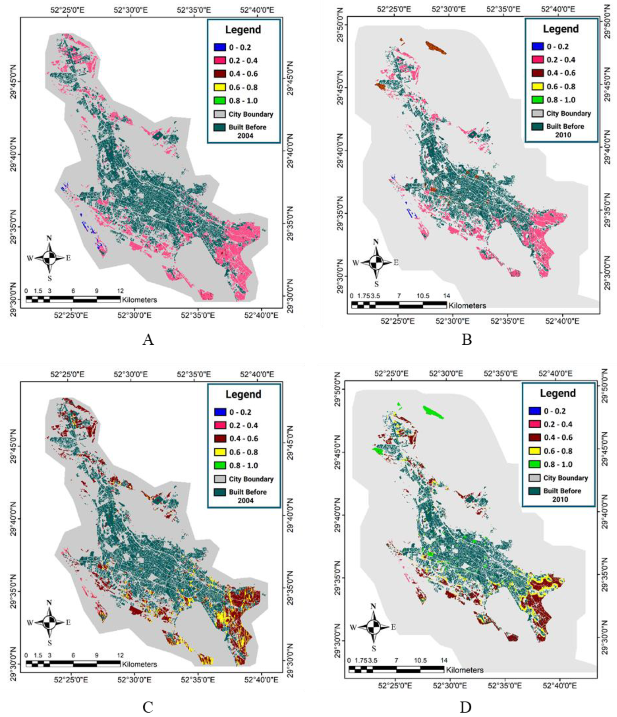
5.4. Determination of Overall Suitability

After the three maps of physical suitability, accessibility suitability, and neighborhood effect were generated, they were integrated in order to obtain the overall suitability. For this purpose, we used the OWA method with four quantifiers and a fuzzy inference engine method. Thus, a total of five maps of overall suitability were produced, the results of which are presented in Figure 8, Figure 9 and Figure 10. The OWA method with Few, Half, and Most quantifiers was used to obtain the weight vectors for the integration of physical suitability, accessibility, and neighborhood effect maps (n = 3):

W_Few = (0.8960, 0.0643, 0.0397)

W_Half = (0.3333, 0.3333, 0.3333)

W_Most = (1.69×10^–5, 0.0173, 0.9826).

Additionally, the weight vector values at each point were different for the Majority quantifier because they are dependent on the values of physical suitability, accessibility, and neighborhood effect of that point. It is worth noting that physical suitability and accessibility maps are common for all of the four quantifiers, i.e., Few, Half, Most, and Majority, but the neighborhood effect map is selected in accordance with each quantifier.

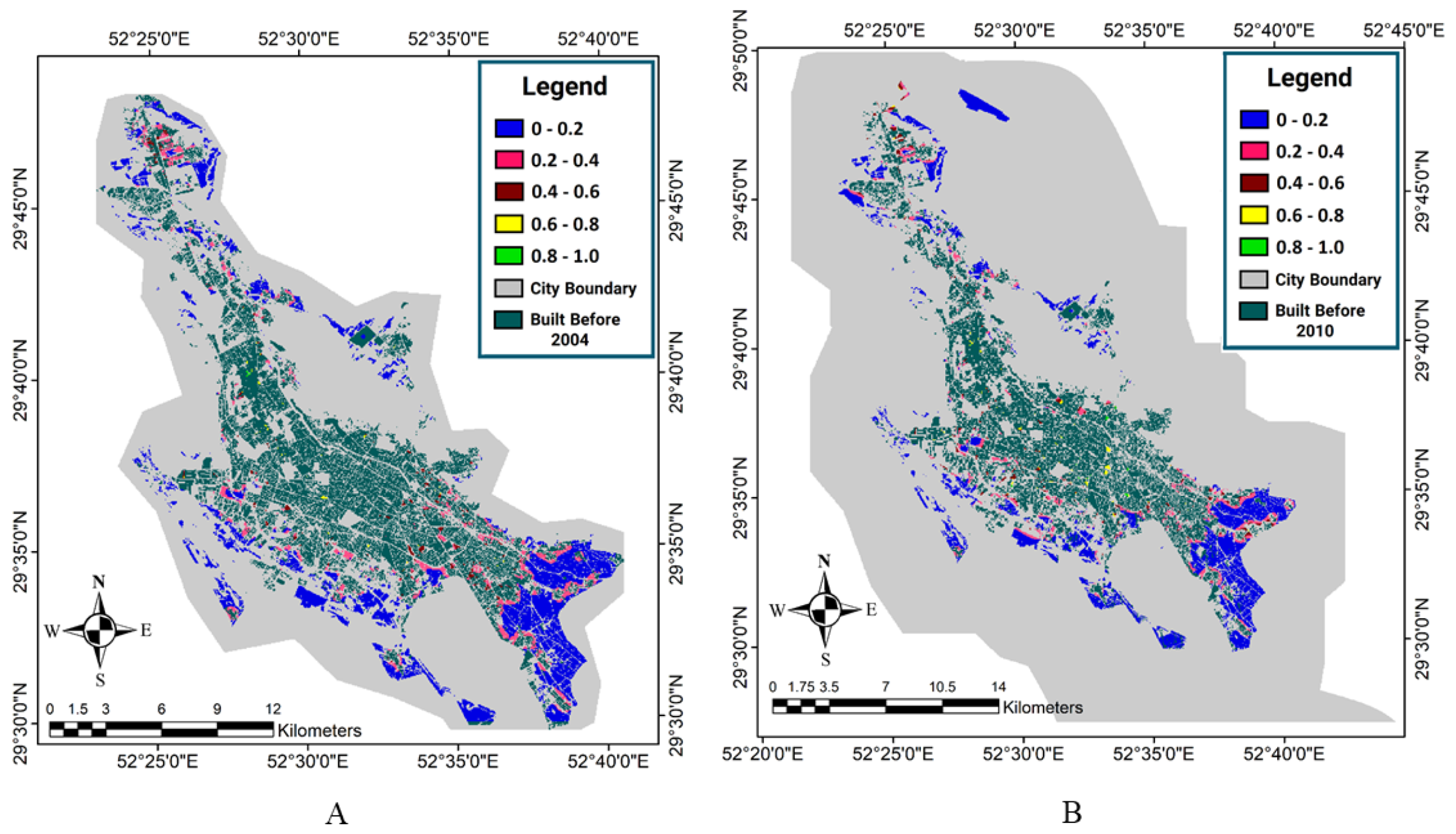
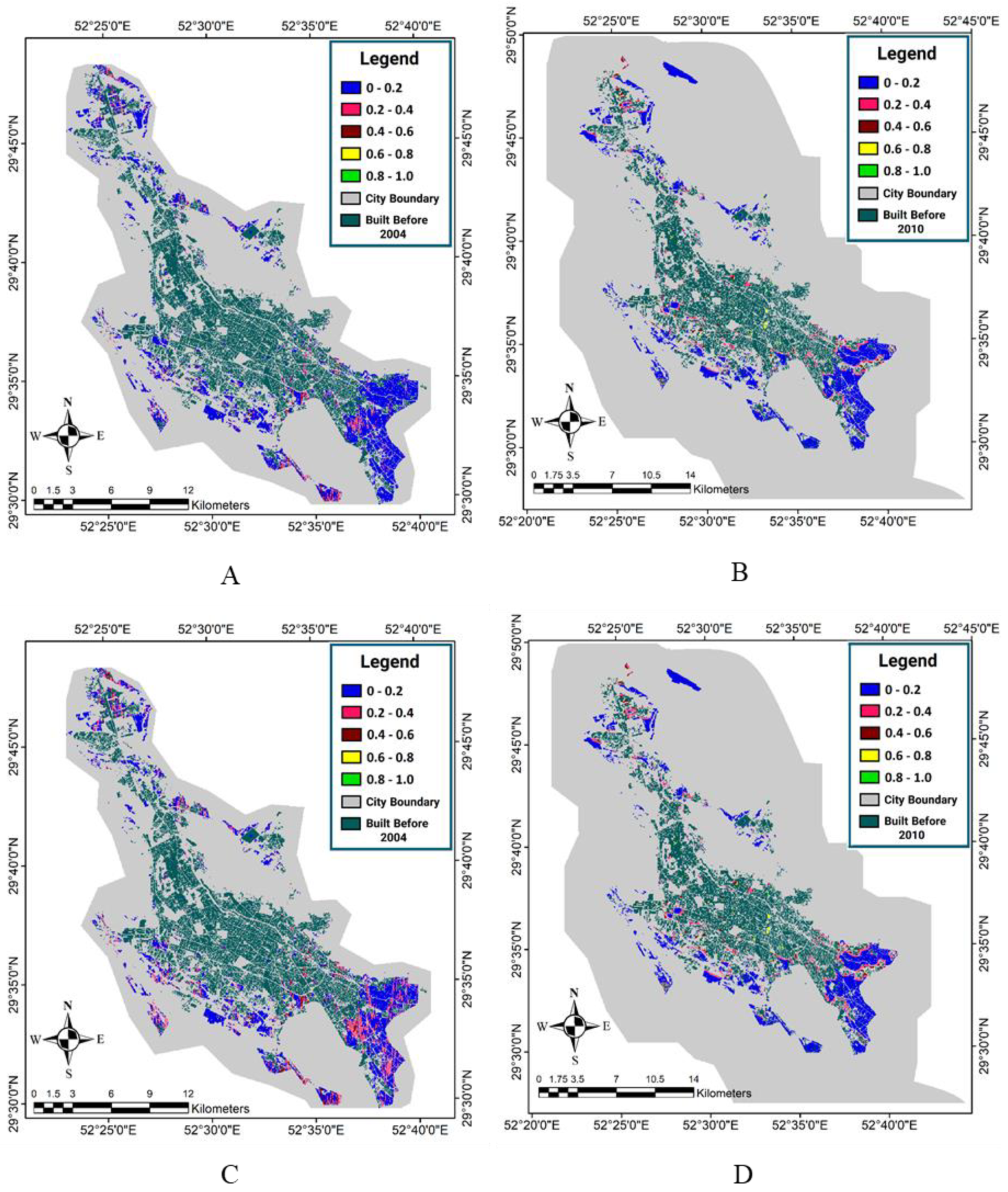
5.5. Model Calibration and Evaluation of Results

As described in Section 4.5, in order to determine the suitable values for the Th₁ threshold, the changes in the values of the accuracy index were examined for that threshold. In this study, the Kappa coefficient was used as the indicator of the accuracy of conformity between the estimated and the reference maps of the developed areas in the first time period. The best values to be chosen for the Th₁ threshold in the first time period were extracted for each of the methods used, and the results are presented in

Table 5. The best values to be chosen for the th₁ threshold in the first time period (2004–2010) to calibrate the different methods used.

No.	Type of Evaluation Index	Methods Used to Identify the Developed Areas
		Fuzzy	OWA Few	OWA Half	OWA Most	OWA Majority
1	Th1 threshold	0.72	0.81	0.74	0.34	0.65

.

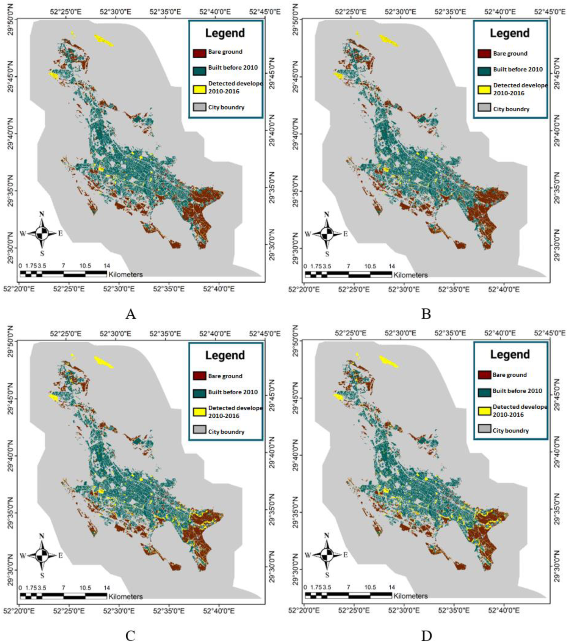
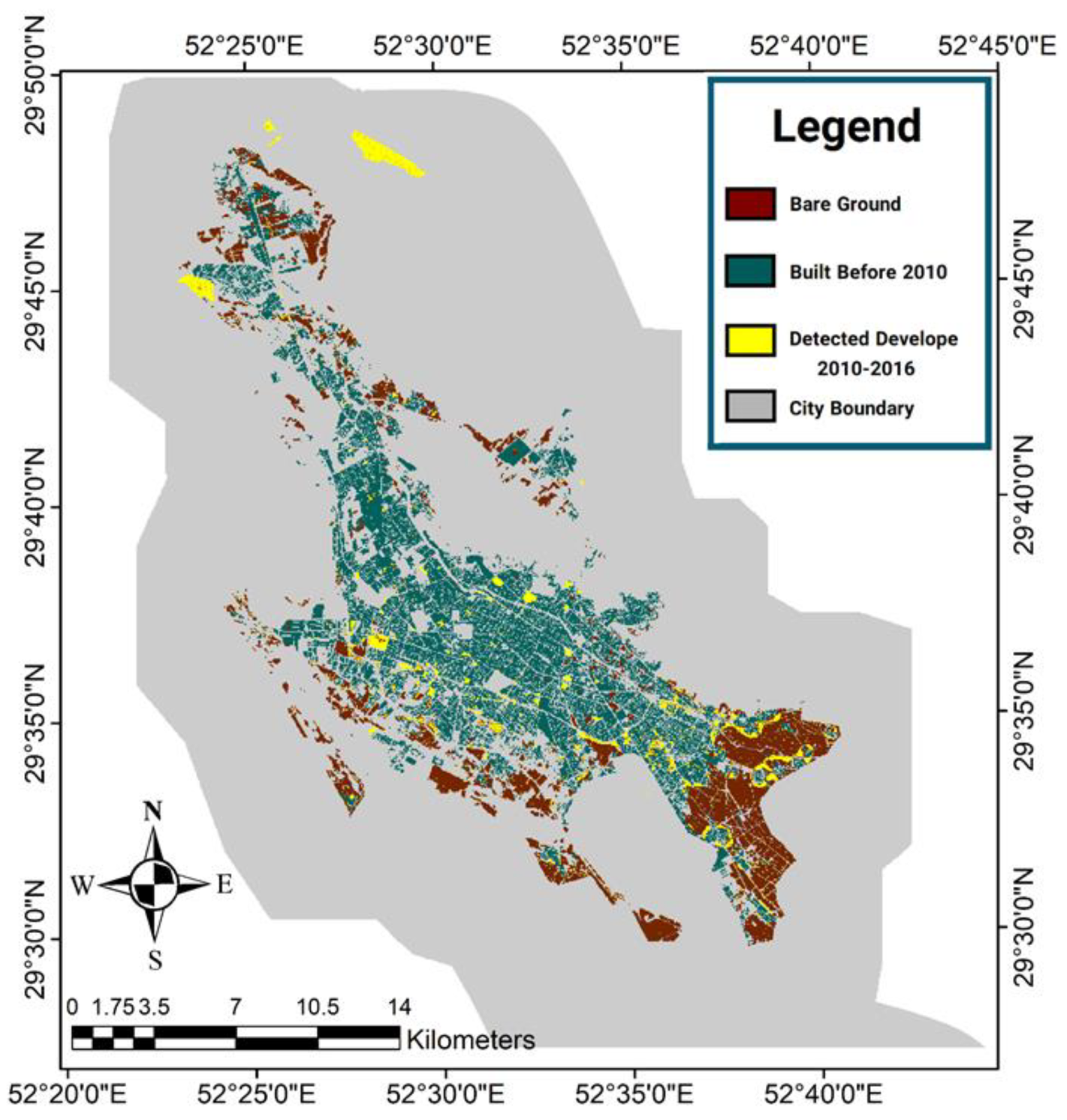
By applying the obtained thresholds from the first time period to the overall suitability maps of the second time period (2010–2016), the forecasted maps of the developed areas in 2016 were generated for different methods. Figure 11, Figure 12 and Figure 13 respectively show the forecasted and reference maps of the developed areas in 2016 for the OWA method quantifiers, the fuzzy interference system, and the reference map of the developed area in the target year. Furthermore, the results of the evaluation methods applied were obtained by comparing the pixel-based forecasted maps and the reference maps of the developed areas in 2016, as presented in

Table 6. Evaluation results of the methods employed to identify the developed areas of Shiraz in the second time period using the calibrated thresholds in the first time period.

No.	Type of Evaluation Index	Methods Employed to Identify the Developed Areas
		Fuzzy	OWA Few	OWA Half	OWA Most	OWA Majority
1	Accuracy of producer	92.57%	57.17%	55.17%	94.34%	99.68%
2	Accuracy of uses	98.45%	100.00%	100.00%	98.07%	97.48%
3	Kappa coefficient	94.22%	67.74%	65.94%	95.16%	98.17%
4	Overall accuracy	98.10%	90.87%	90.44%	98.40%	99.38%

. It is worth noting that in this evaluation, the areas that are built-up in 2016 and were not bare grounds in 2010 either were not considered, because the model was designed to estimate the changes from the bare ground use in the baseline year (2010) into the built-up areas in the target year (2016).

The evaluation results indicated that, compared to the other methods, the OWA-Majority method had the most accurate values in the accuracy of the producer, Kappa, and overall accuracy. It was also observed that the fuzzy inference system, OWA-Most, and OWA-Majority had a high accuracy in identifying the developed areas in the target year (2016). However, due to a lower detection of the developed pixels, the OWA-Few and OWA-Half methods caused an increase in the FN values and a decrease in the accuracy of the producer and the Kappa coefficient. Thus, the thresholds obtained in the first time period for these two methods were higher than the best threshold values in the second time period. The areas of the reference built-up areas and the developed areas in the second period are presented in

Table 7. Reference areas of built-up and developed areas by five applied methods in the second period.

No.	Type of Area	Second Time Period (2010–2016)
1	The reference area of built-up areas before 2010	9247.05
2	The reference area of bare grounds in the baseline year (2010)	6099.6
3	The reference area of built-up area between baseline and target years	1299.9
4	Estimated area of the built-up areas using the fuzzy inference system	1222.3
5	Estimated area of the built-up areas using the OWA-Few method	743.2
6	Estimated area of the built-up areas using the OWA-Half method	717.2
7	Estimated area of the built-up areas using the OWA-Most method	1250.5
8	Estimated area of the built-up areas using the OWA-Majority method	1329.3

. Based on the table, the OWA-Majority method had the closest estimation to the reference level of the developed areas. The results confirmed that the developed areas in the OWA-Few and OWA-Half methods were less than in the reference level. Additionally, we compared the presented method with other methods to show the efficiency of the proposed method in identifying the developed areas. Shafizadeh-Moghadam [21] applied Logistic Regression (LR), Random Forest (RF), medium ensemble forecasting, and ANN models to simulate urban growth in Tehran, Iran. They used 1985–1999 data and 1999–2014 data to calibrate and validate the model, respectively. They calculated the overall accuracy to show the efficiency of the proposed models in detecting the changed and unchanged cells, which achieved 80.5%, 79.3%, 78.4%, and 80.66% for the ANN, RF, LR, and medium ensemble models, respectively. Chan et al. [32] used various machine learning methods such as Maximum Likelihood (ML), Decision Tree (DT), Learning Vector Quantification (LVQ), and Multi-layer Perceptron (MLP) algorithms to identify the growth and changes of urban areas. They calculated the OA metrics to show the effectiveness of the suggested approaches in detecting, which were 70.83%, 84.50%, 88.08%, and 73.25%, respectively. The results showed that LVQ did better and was the best performer in detecting the urban environment growth and changes. Liu et al. [41] analyzed land-use suitability for urban development in Beijing, China based on two multi-criteria approaches, the OWA and Ideal Point (IPM) methods. They obtained a Kappa index and OA of 78% and 91% respectively, which showed that these two techniques present very comparable dispensations of spatial land-use suitability in addition to performing well in analyzing the urban growth, whereas the results obtained in the present study for overall accuracy are 98.10%, 90.87%, 90.44%, 98.40%, and 99.38%, respectively, for the Fuzzy, OWA-Few, OWA-Half, OWA-Most, and OWA-Majority methods. The results suggest that, compared with the other methods mentioned, the methods proposed in this study are more effective in identifying the developed areas and modeling urban growth.

6. Conclusions

In this study, a method was proposed to forecast the changes of bare ground into developed or built-up areas by using fuzzy concepts and ordered weighted averaging (OWA) methods. Then, the proposed model was calibrated for the development of bare grounds into built-up areas in the first time period and applied to the data of 2010, providing the map of bare grounds changed into built-up areas for 2016. In this study, the results of different methods were compared with each other and with reality. The results indicated that the OWA-Few and OWA-Half methods were not successful in forecasting changes from bare grounds into built-up areas, while the fuzzy inference system, OWA-Most, and OWA-Majority methods had very good results, as in these three methods, all indices had high accuracy. In other words, in addition to the comprehensive identification of the unchanged and developed pixels (high TP and TN), they also identified the unchanged and developed pixels as correctly as possible (low FP and FN) and increased the Kappa, user accuracy, and producer accuracy indices. The OWA-Majority method had the highest accuracy, and its complexity and computational costs were higher than those of the other methods. On the other hand, the advantage of the OWA-Majority method over the fuzzy EF method lies in its decisiveness and its non-dependence on user-defined parameters. Thus, there is a lower possibility of a human error in this method. Furthermore, the results obtained from the two methods of the fuzzy inference system and OWA-Most indicated their similarity, which may be due to the stringency in the rules defined for the fuzzy system rule bases in integrating the physical suitability, accessibility, and neighborhood effect maps. However, the proposed method has some limitations as well. One of the main limitations of the proposed method is that it could not predict the areas that are built-up in 2016 and were not bare ground in 2010. In other word, the proposed model was not able to model the areas that were not bare ground in 2010 and were subsequently converted into bare ground and then again into built-up areas in 2016. In addition to that, the method could not model the built-up areas in the suburbs that did not comply with the building standards and did not consider any of the effective parameters mentioned, Finally, the fuzzy inference system, OWA-Most, and OWA-Majority methods were successful in forecasting the areas changed from bare ground into developed areas and could be used to forecast the level and location of changes from bare ground into developed use over the next six-year period.