Seismic Fragility Analysis of Tunnels with Different Buried Depths in a Soft Soil

Department of Disaster Mitigation for Structures, Tongji University, Shanghai 200092, China
*
Author to whom correspondence should be addressed.
Sustainability 2020, 12(3), 892; https://0-doi-org.brum.beds.ac.uk/10.3390/su12030892
Submission received: 3 January 2020
/
Revised: 22 January 2020
/
Accepted: 22 January 2020
/
Published: 24 January 2020
(This article belongs to the Special Issue Geo-Hazards and Risk Reduction Approaches)
Abstract
:Seismic fragility of an engineering structure is the conditional probability that damage of a structure equals or exceeds a limit state under a specified intensity motion. It represents the seismic performance of structures and the correlation between ground motion and structural damage, playing an indispensable role in structural security assessment. A practical evaluation procedure of acquiring the fragility curves of tunnels in a soft soil has been proposed in this paper. Taking a typical metro tunnel in Shanghai as an example, two-dimensional finite element models of soil-tunnel cross-section were established. The nonlinear characteristics of soil layers were considered by the one-dimensional equivalent linear analysis in the equivalent-linear earthquake site response analyses (EERA) program. The ground motions were selected based on seismic station records. Comparing the analytical fragility curves with the empirical curves derived from American Lifelines Alliance (ALA) and HAZUS shows that the proposed method is reliable and feasible. Further study about the influence of buried depths on the fragility of the tunnel was performed. The results indicate that the failure probability of the tunnel is not monotonically decreasing with the increase of the buried depth for a given peak ground acceleration (PGA.)
1. Introduction
An earthquake is a serious natural disaster that constitutes a threat for urban infrastructure and people’s life. People have insufficient understanding about seismic resistance of underground structures. It is generally believed that an underground structure is much safer than a ground structure because of smaller deformations under the condition of surrounding rock or soil constraints. Since the 1990s, many devastating earthquakes causing serious damage to subway stations and tunnels have occurred, such as the Kobe earthquake, Chi-Chi earthquake and Wenchuan earthquake, which means that underground structures are still susceptible to damage under severe earthquakes. According to actual cases of tunnel failure, it has been obtained that shallow tunnels and tunnels built in the unfavorable geological layer are more vulnerable [1]. Meanwhile, it is very difficult to repair when the tunnel is seriously damaged. Therefore, analyzing the seismic vulnerability of tunnels is necessary.
Seismic fragility of engineering structures is the conditional probability that damage of a structure equals or exceeds a limit state under a given seismic input ground motion. It not only quantitatively represents the seismic performance of engineering structures from the probability, but also describes the relationship between the intensity of ground motion and the degree of structural damage from the macro perspective. The vulnerability assessment of tunnels has been mainly based on empirical fragility curves or expert judgments [2,3,4]. American Lifelines Alliance (ALA) and the organizing committee of HAZUS system obtained empirical fragility curves of tunnels for different types of materials and soil conditions by regression analysis based on a worldwide damage database. They have the statistical average significance. Recently, with the application of finite element software, numerical simulation has been widely used in seismic fragility analysis [5,6,7,8,9,10,11]. Additionally, the fragility analysis method has been optimized and evaluated in the application [12,13,14]. Although the numerical simulation method has been used to produce the seismic fragility of tunnels [15,16,17], especially in areas where the damage data are unavailable, the application on tunnels is still scarce compared to buildings and bridges.
Buried depth is a signification factor affecting seismic vulnerability of tunnels. Sharma et al. found that underground structures with a depth less than 50 m are more vulnerable to damage through investigation and statistics on 132 cases of earthquake damage [18]. Gao et al. conducted simulation analysis and the shaking table test for a large number of tunnels with different buried depths, and preliminarily presented the variation rule of tunnel lining stress with buried depth [19]. Choosing reasonable burial depth cannot only minimize the impact of potential earthquakes on the tunnels, but also save the construction cost to a large extent.
Based on the research of tunnel seismic vulnerability, this paper aims to obtain a practical evaluation method of the fragility curves of tunnels in soft soils, considering different buried depths. The comparison between the analytical fragility curves and the empirical ones confirms the rationality of the former. Further analysis to study the law of fragility curves about buried depth could be carried out.
The response of the tunnels under earthquakes could be considered separately along the axis of the tunnel and the transverse direction of the tunnel. The seismic response of the cross-section of the tunnels is the focus of this research. For this purpose, the state of the surrounding soil of the tunnel is needed. The equivalent linear analysis proposed by Seed et al. [20] is widely used in free-field soil response analysis because of its simple principle, convenient parameters acquisition, small calculation and certain reliability. However, it has the following shortcomings: the calculation results are unreasonable when the input motion is large and the soil is soft; the error of results in high frequency range is large; an endless loop may appear in the calculation; and it has obvious resonance effect [21].
Taking a typical engineering tunnel in Shanghai as an example, two-dimensional refined finite element models of soil-tunnel cross-section were established in ABAQUS [22], which belongs to Dassault Systemes Simulia Corp. whose headquarters is in Providence, Rhode Island, USA, and the nonlinear characteristics of soil layers were considered through the one-dimensional equivalent linear analysis with the equivalent-linear earthquake site response analyses (EERA) program [23], to explore the influences of the above factors on seismic vulnerability of tunnels.
2. Seismic Fragility Analysis Methodology of Tunnels
2.1. Procedure of Seismic Fragility Analysis
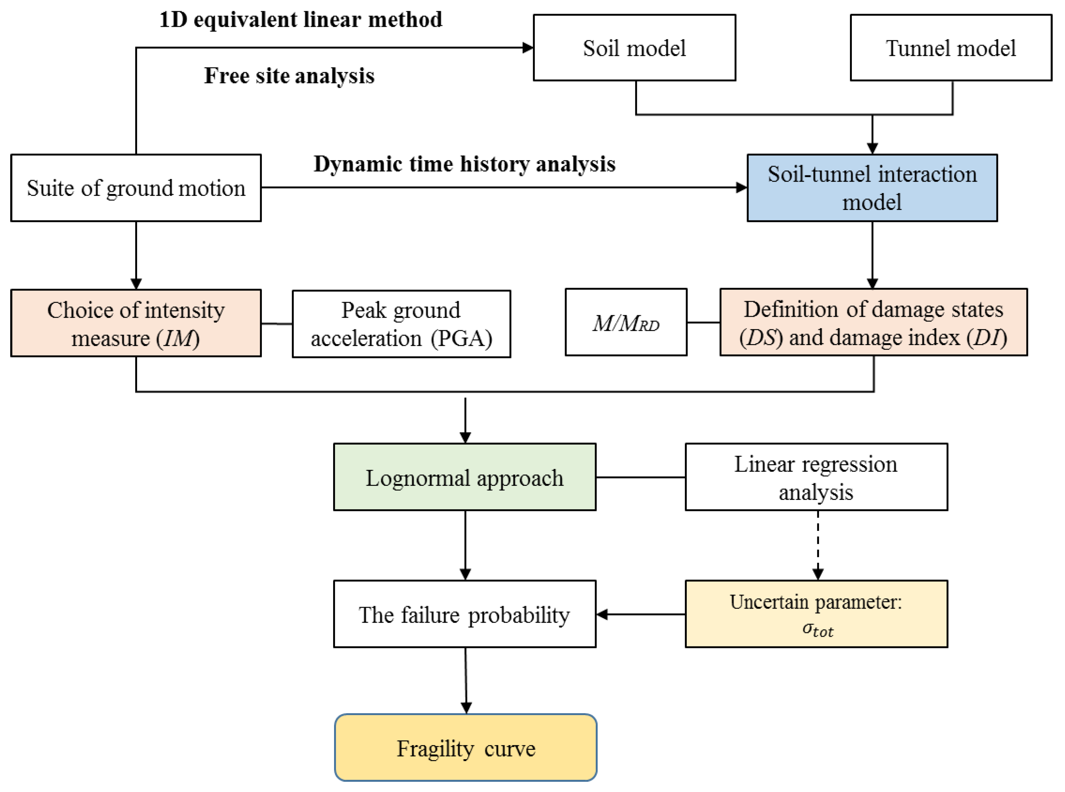
The procedure of seismic fragility analysis is shown in Figure 1. More details of key steps are given in the following processes:
- The suite of applicable ground motion is chosen for analysis according to the site information.
- Free site response analysis is conducted through a 1D equivalent linear analysis on the soil profiles, paired with input motions at different seismic intensity levels, to acquire the dynamic characteristics of soil layers. The nonlinear soil behavior is considered through equivalent shear modulus G and damping ratio ζ compatible with shear strain.
- Establish the finite element soil-tunnel model and evaluate seismic response by dynamic time history analysis in a finite element software such as ABAQUS.
- Selection of the intensity measure (IM) parameter of input ground motions for developing the fragility curves.
- Definition of damage states (DS) corresponding to the damage index (DI) for determining the damage of tunnel lining.
- The damage assessment can be performed based on lognormal approach with linear regression to determine the relationship of DI and IM.
- A lognormal standard deviation (βtot) that describes the total variability associated with each fragility curve must be estimated.
- These outputs are obtained and used for developing the fragility curves of tunnels.
2.2. Intensity Measure (IM) Selection
The peak ground acceleration (PGA), peak ground velocity (PGV), peak ground displacement (PGD) or response spectral acceleration (SA) are usually chosen as an intensity measure for seismic fragility in engineering applications. The PGA that is peak acceleration of input ground motion in the time history is a good index. ALA produced empirical fragility curves by PGA, and PGA is selected as the IM in many tunnel fragility studies [2,5,7,24]. Thus, PGA is adopted as the IM for calculating the conditional probability of tunnel lining failure in this paper.
2.3. Definition of Damage States (DS)
The definition of damage states, which are described by a damage index expressing relationship between the actual response and the capacity of the lining, and selection of corresponding damage indicator, are critical for vulnerability assessment of engineering structures. Generally, responses of structures can be evaluated by engineering demand parameters (EDP), which are useful to predict the damage to structures. Although previous researches have defined various damage indexes employed in seismic fragility analysis of buildings and bridges, such as maximum displacement, the inter-story drift ratio, and stress for evaluating the EDP [25,26], no such information is available for tunnels. In the process of developing empirical fragility curves, the damage states of tunnels are often divided based on the damage degree of tunnels in past earthquakes. The process of deriving numerical fragility curves is inconsistent with the empirical curves.
Based on the common failure modes of tunnels, the damage index is defined as the ratio of the actual (M) and the capacity (MRD) bending moment of a tunnel cross-section, according to some existing studies [15,27]. The mechanical behavior of a tunnel lining is simulated by an elastic beam subjected to deformations imposed by the oscillating surrounding ground due to seismic waves propagating perpendicular to the tunnel axis. The actual bending moment is calculated by the dynamic time history analysis. The capacity of the bending moment can be obtained by considering the materials and geometry properties of the tunnel section. Five different damage states are determined, namely, none, minor, moderate, extensive and collapse. The damage states and corresponding damage index are shown in Table 1.
2.4. Derivation of Fragility Function
Many engineering structural fragility studies show that the following relationship is satisfied between the structural engineering demand parameter (EDP) and the ground motion parameter (IM):
where the and are regression parameters.
Median value of damage index is a special structural engineering demand parameter. The following exponential relationship between and IM can also work:
Taking the logarithm on both sides of the above Equation (2), thus:
The above parameters can be calculated by the data of finite element analysis and obtained by linear regression.
The currently applied approach consists in response function of structures obeying lognormal distribution, that is:
where , are the logarithm median and logarithm standard deviation of EDP, respectively.
Similarly, the probability function of the capacity (C) of structure can also be expressed by lognormal distribution function. Therefore, the function can also be expressed by two parameters and as follows:
where and are the logarithm median and logarithm standard deviation of C, respectively.
Seismic fragility curve of structures is a statistical tool representing the conditional probability that structural response EDP exceeds the capacity (C), defined by the damage states given a specified intensity level (IM), and it is expressed in the following equation [4,5,28]:
The Equation (6) can be rewritten as . Setting , with statistical parameter Z that represents the state function of structures which also obeys normal distribution. It is easy to calculate the average value and standard deviation of Z, which are , , separately. Therefore, the failure probability of the structure conditioned on ground motion parameter can be expressed as:
For the convenience of calculation, the should be transformed into a standard normal distribution . Setting , and then the new equation of the failure probability is:
where the is the probability of being equal to or exceeding a particular damage state for a given seismic intensity level; is the standard cumulative probability function; is the median threshold value of the capacity required to reach the particular damage state that can be obtained by looking up in Table 1; the parameter describes the uncertainty caused by the capacity of tunnels, and based on HAZUS for building [4]; the parameter is caused by the EDP, and according to analyses for bored tunnels of BART system [29].
Some experts suggest that be replaced by the total variability to calculate the probability of a tunnel’s failure, which is reasonable in the vulnerability assessment of a tunnel [4,15,16]. The modified fragility function is:
where describes the total variability associated with each fragility curve, and
where is the standard deviation caused by the uncertainty of other factors related to vulnerability assessment, being usually determined by calculating natural logarithmic standard deviation of damage index (DI) for the different input motions at each level of PGA [4].
3. Numerical Model of Soil-Tunnel System
3.1. Specification of Tunnel Lining
This research takes a prototype of a subway tunnel in Shanghai whose essential parameters are known to conduct the seismic vulnerability assessment [30]. The tunnel with a double-hole of a 13 m center distance is considered. The shape of the tunnel lining section and its parameters are displayed in Figure 2. The section of the hole is circular, and its outer diameter is 6.2 m. The thickness of the tunnel lining is 0.35 m. The tunnel is made of concrete, and the material properties are as follows: Young’s modulus E = 34.5 GPa, Poisson ratio v = 0.2. The buried depths chosen are 10 m, 15 m, 20 m, 35 m, respectively, to explore the variation of the tunnel lining vulnerability with buried depth. To express the key points of the lining clearly later, the section has been simplified, as shown in Figure 2.
3.2. Soil Profile
The selected site is a deep soft soil site with rock formations at about 280 m depth [31]. The entire soil profile is mainly composed of clay and sand, which could be divided into 14 soil layers and 6 soil materials (see Table 2) in analysis. The shear wave velocity and density of soil layers are shown in Figure 3.
The nonlinear characteristics of soil layers are considered by one-dimensional equivalent linearization method, to obtain equivalent shear modulus ratio G/Gmax and damping ratio ζ compatible with equivalent shear strain. Before applying the method, the soil dynamic parameters must be defined, collected from lots of experimental results that are the variations of shear modulus ratio G/Gmax and damping ratios ζ with shear strain, as listed in Table 2 [32]. The maximum shear modulus Gmax of soil layers should be estimated by shear wave velocity and density , namely the following equation:
The equivalent shear modulus ratio G/Gmax and damping ratio ζ are calculated by EERA which is an iterative computational program based on SHAKE91, paired with input motions at each of the seismic intensity levels. In the iterative procedure, the ratio of the effective and maximum shear strain is assumed equal to 0.65. The results can be converted into elastic modulus and Rayleigh damping of the soil-tunnel model, and then the dynamic time history analysis can be carried out.
The free field response analysis is a key step in the analysis of soil-structure interaction for underground structures [33]. Figure 4 shows a typical example of the computed ground response in terms of equivalent shear modulus ratio G/Gmax, equivalent damping ratio ζ, peak acceleration and peak shear strain . The computed value at the soil surface (PGA) is selected as the seismic intensity parameter in the fragility curves.
3.3. Establishment of Soil-Tunnel Model and Boundary Condition
The finite element models (FEM) of the two-dimensional soil-tunnel system is generated using the software ABAQUS to calculate the actual internal forces (including the moment and the axis force) of the lining under the excitations of vertically propagating shear wave. The soil-tunnel model with a 2800 m width and a 280 m depth is displayed in Figure 5. Considering that the longitudinal length of the tunnel is much larger than the cross-section size, the soil and tunnel lining are simulated by plane-strain element and beam element, respectively. The grid size satisfies the size control conditions proposed by Kuhlemyer et al. [34]; that is, the maximum side of each element is less than 1/8 wavelength corresponding to the maximum frequency. To obtain an accurate model, the model should be composed closely with the real behavior of the soil-tunnel interface. Therefore, the area around the tunnel is more finely meshed. The four buried depths of the tunnel are 10 m, 15 m, 20 m, and 35 m. Four soil-tunnel models are established. Each model consists of more than 170 thousand elements.
The bottom boundary condition for the soil domain is fully fixed at the base. The lateral boundaries could dissipate the arriving scattered waves. Building a sufficiently large soil domain (2800 m × 280 m) could dissipate the waves. Constraining the boundary nodes to move in pure shear is to simulate a free-field condition. The pure shear constraint can be achieved by ensuring the nodes at the lateral boundaries at the same elevation to move together horizontally [35,36], also called the periodic boundary. The periodic boundary is applied to the model and keeps compatible deformation.
3.4. Selection of Input Ground Motions
Selection of ground motions is significant for seismic fragility analysis; it is not only to ensure adequate quantity, but also to meet site characteristics. Although the strong motion observation network has been set up in Shanghai, the strong motion records have not been obtained so far. Thus, the required seismic waves can only be selected from the existing records. Fifteen ground motions with different intensities are selected from the Pacific Earthquake Engineering Research Center (PEER) by the method based on the station/earthquake information [37,38] listed in Table 3, and the response spectrum of the input motions is shown in Figure 6. The criteria for selecting seismic waves are as follows:
- In reference to Chinese codes for seismic design of buildings, the seismic wave whose shear wave velocity Vs_30 m is less than 200 m/s is selected firstly.
- To reduce the effect of near-field effects, the epicentral distance of the selected seismic waves must be more than 10 km.
- To avoid the influence of the same focal mechanism, only one horizontal seismic wave is selected for each station and each seismic event.
- To avoid the dependence of the selected seismic waves on the recording direction, only one of the larger PGA is selected for the two horizontal time history recording curves of the same seismic event.
- Fifteen different seismic waves are selected, and the seismic waves with larger magnitudes are prioritized in the wave selection process to eliminate the earthquake that is unlikely to affect structural safety.
The waves are input at the bottom of the model, so the selected surface ground motions need to be performed by an inverse analysis to obtain the bedrock waves as the input. Meanwhile, to acquire the internal forces of the tunnel lining for gradually increasing level of seismic intensity, the peak of time histories is, in turn, scaled into 0.03 g, 0.075 g, 0.15 g, 0.3 g, 0.45 g, 0.6 g, 0.75 g, 0.9 g, 1.05 g and 1.2 g. The principle is that the frequency characteristics before and after amplitude modulation is consistent.
4. Fragility Analysis with Different Buried Depths
4.1. Internal Forces and Deformation of the Lining
The weak position can be estimated by investigating the response distribution along the circumferential direction of the lining structure under earthquake excitations. Meanwhile, the bending moment is an important index of the tunnel damage state in the fragility analysis. Linear elastic analysis was carried out by using ABAQUS software. The internal force distribution was studied with changing the buried depth of tunnels and the peak acceleration of ground motion. It was found that most of the results showed the similar trend. The variation trend of bending moment and axial force with different buried depths under the excitation of Northridge-01 wave (0.15 g and 0.60 g) is illustrated in Figure 7. The peak values of the bending moment and the axial force of the circular tunnel lining always appear near the four positions having a 45° central angle with the connecting line of the dome (point A) and the arch bottom (point E), corresponding to θ = 45°, θ = 135°, θ = 225°, and θ = 315°. It also can be seen that the bending moment increases first and then decreases with the increase of burial depth, and that the peak occurs when the depth is 15 m. However, the axial force of the tunnel increases with the increase of the buried depth.
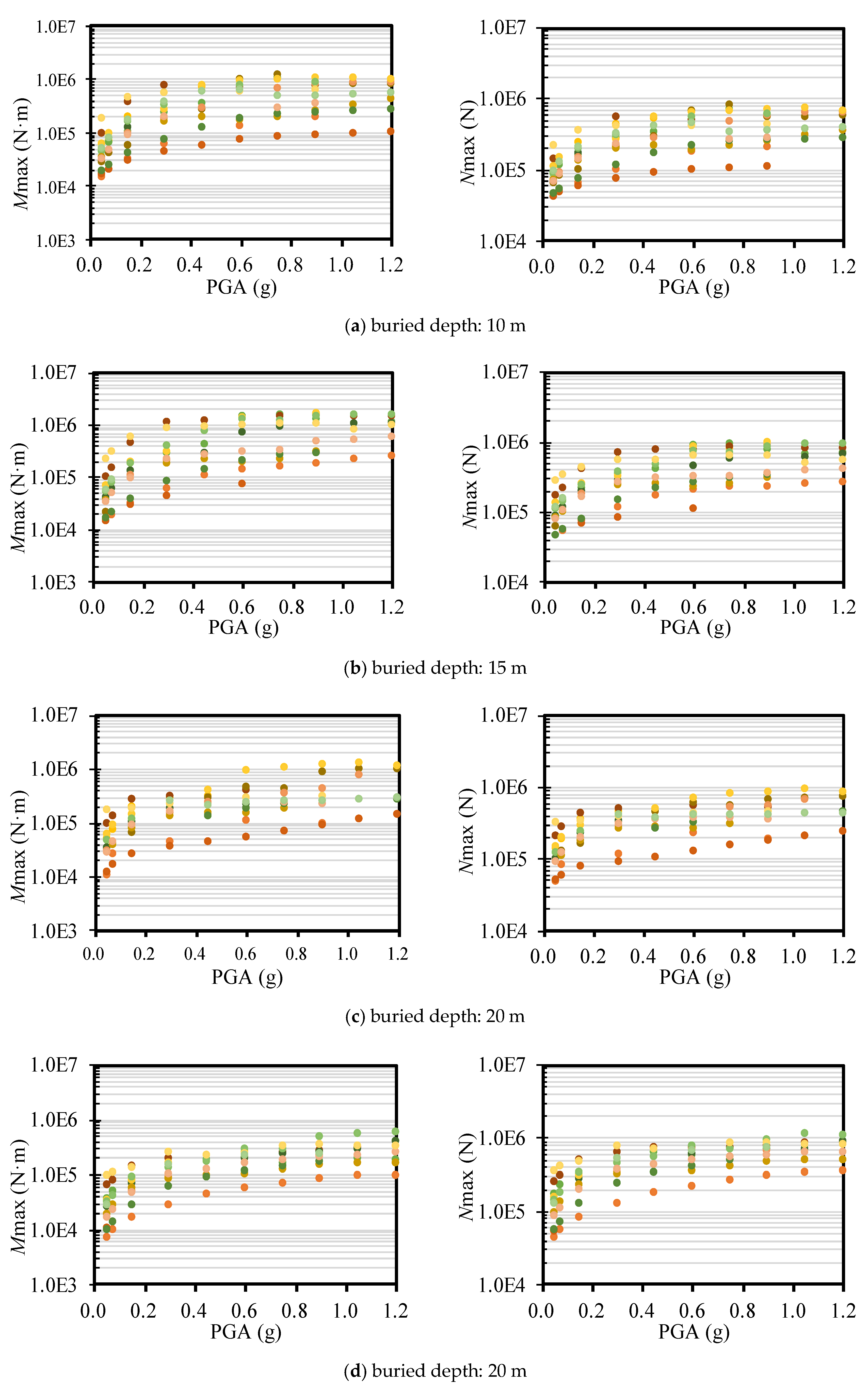
Figure 8 displays the response trend of the tunnel lining under the earthquake waves with different PGA. Intuitively, the and increase with the increase of PGA under the same wave, and the increasing trend starts being slow or no longer exists when PGA is greater than 0.9 g. Besides, the dispersion of axial force reaction is less than that of moment reaction.
The failure of the tunnel is mainly caused by the overlarge deformation based on the statistical analysis of seismic damage data of lining. To further explore the relationship between structural deformation and forces, the correlation of the relative displacement between point A and point E in Figure 2 and bending moment were fitted, as shown in Figure 9. There is a linear correlation between them according to Figure 9. So, selecting bending moment as the damage index is compatible with the use of the deformation. Therefore, it is feasible to take the moment as the damage index when the deformation index is difficult to determine in seismic fragility analysis.
4.2. Seismic Fragility Curves with Different Buried Depths
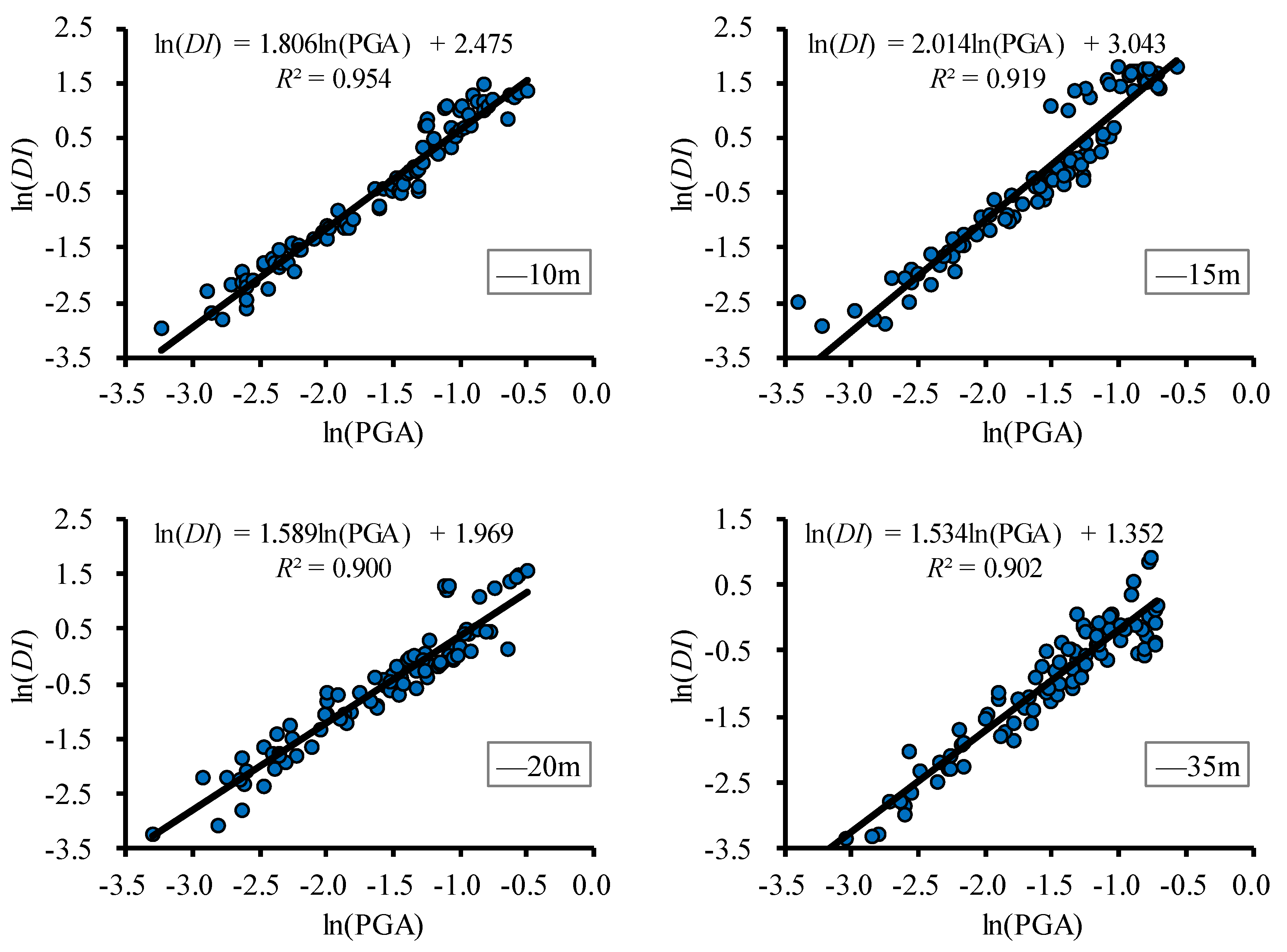
The correlation between DI and PGA must be determined before the fragility curve could be obtained. Through a series of dynamic time-history analysis of the soil-tunnel system, the maximum bending moment of the lining with four buried depths can be acquired. Thus, the DI () can also be calculated. DI is a special structural engineering demand parameter (EDP), and PGA is selected as the intensity measure (IM) for the analysis. Therefore, DI and PGA satisfy the following formula:
The correlation between DI and PGA is determined by linear regression analysis, as shown in Figure 10. The goodness-of-fit (R2) of all results are better than 0.9, which means the discreteness of results is relatively small, and that fitting results are satisfactory. This may be related to the wave selection method based on the station/earthquake information that will reduce the dispersion of calculation results according to Reference [37].
The logarithmic standard deviation of damage index (DI) for the different input motions at each level of PGA can be calculated from the regression results, which means that the could be estimated, as illustrated in Table 4.
After acquiring the correlation between DI and PGA and the total uncertainty , they could be taken into the fragility Equation (9) to calculate the failure probability of the tunnel lining for a given seismic intensity level. Thus, the formulas of the tunnel fragility for the different buried depths are:
where Equations (13)–(16) refers to the buried depth of 10 m, 15 m, 20 m and 35m, respectively.
The fragility curves of the tunnel are shown in Figure 11. It can be seen that, for the tunnels with the four depths in Shanghai soft soil, the tunnel with 15 m buried depth is most vulnerable to earthquake and 35 m buried depth is least vulnerable at a given PGA. Therefore, the failure probability of the tunnel is not monotonically decreasing with the increase of the buried depth. The maximum deformation of the soil layer appears in the 15 m depth case, shown in Figure 4. In general, the reason for this phenomenon is related to the deformation due to a small equivalent shear modulus and a large damping ratio. The greater the deformation of the soil layer, the greater the internal force generated.
4.3. Comparison Between Numerical and Empirical Fragility Curves
Empirical fragility curves could be obtained based on the history seismic damage data, which can reflect the actual damage of structures. However, empirical fragility curves do not always perform well for a city lacking strong seismic records. Meanwhile, the acquisition of the empirical fragility curves does not take into account specific soil characteristics, tunnel depth, tunnel material information, and so on. However, it is still instructive. The analytical fragility curves obtained in this study and the empirical fragility curves derived from ALA and HAZUS are compared in Figure 12 [2,4]. It can be seen that only the analytical fragility curves of the tunnel with 35 m depth are close to the empirical fragility curves of HAZUS. The empirical fragility curves are often statistically averaged. The shallow metro tunnel in Shanghai soft soil is easy to cause unexpected responses. Then, the curve of the tunnel with a larger buried depth is consistent with the empirical one. The intensity level corresponding to the failure probability of 50% is defined as the median PGA, and the median PGA is listed in Table 5.
5. Conclusions
The empirical fragility curves always have the statistical significance, ignoring specific soil characteristics, buried depth and tunnel material. A numerical method of performing the fragility assessment of the metro tunnel which can effectively avoid the defects has been proposed in this paper. The benefit of the proposed method is that it can provide a basis for seismic fragility analysis of tunnels without strong seismic records. Two-dimensional finite element models of a typical metro tunnel with four buried depths were built by using ABAQUS. The nonlinear characteristics of soil profiles were considered by one-dimensional equivalent linear method. The input ground motions were selected by the method based on station/earthquake information. A series of dynamic time-history analysis were carried out.
The bending moment is an important index of describing the tunnel damage state. According to the distribution of , the maximum of the lining always appears near four positions that are θ = 45°, θ = 135°, θ = 225° and θ = 315°. There is a linear correlation between and tunnel relative deformation. Selecting bending moment as the damage index is compatible with the use of deformation. Therefore, it is valid to take the moment as the damage index when the deformation index is difficult to determine in seismic fragility analysis. The correlation between damage index and PGA is determined by linear regression. The goodness-of-fit results are satisfactory, which means the discreteness of results is relatively small. This may be related to the method of wave selection based on the station/earthquake information that will reduce the dispersion of calculation results.
Comparing the analytical fragility curves and the empirical curves derived from ALA and HAZUS indicates that the proposed method is reliable. Further analysis about the effect of buried depth on the fragility of the tunnel has been performed. The results show that the failure probability of the tunnel is not monotonically decreasing with the increase of the buried depth for a given PGA, and that the tunnel with 15 m buried depth among the four depths is most vulnerable to earthquake, which is related to the overlarge deformation of soil layers at 15 m depth due to a low equivalent shear modulus and a high equivalent damping ratio.
Author Contributions
Conceptualization, Z.Z.; methodology, Z.Z.; software, Y.R.; investigation, Y.R.; data curation, H.C.; writing—original draft preparation, H.C. and X.H.; writing—review and editing, X.H. All authors have read and agreed to the published version of the manuscript.
Funding
This research and the APC was funded by the National Natural Science Foundation of China, grant number 51778491.
Acknowledgments
The authors gratefully acknowledge the financial supports from the National Natural Science Foundation of China, grant number 51778491.
Conflicts of Interest
The authors declare no conflict of interest.
References
- Zheng, Y.L.; Yang, L.D. Earthquake damages and countermeasures of underground structures. Earthq. Resist. Eng. 1999, 4, 23–28. (In Chinese) [Google Scholar]
- American Lifelines Alliance (ALA). Seismic Fragility Formulations for Water Systems, part 1—Guideline; ASCE-FEMA: Reston, VA, USA, 2001. [Google Scholar]
- Applied Technology Council-ATC-13. Earthquake Damage Evaluation Data for California; Applied Technology Council: Redwood City, CA, USA, 1985. [Google Scholar]
- National Institute of Building Sciences (NIBS). HAZUS-MH: Technical Manuals; Federal Emergency Management Agency and National Institute of Building Science: Washington, DC, USA, 2004. [Google Scholar]
- Kappos, A.; Panagopoulos, G.; Panagiotopoulos, C.; Penelis, G. A hybrid method for the vulnerability assessment of R/C and URM buildings. Bull. Earthq. Eng. 2006, 4, 391–413. [Google Scholar] [CrossRef]
- Lu, X.Z.; Shi, W.; Zhang, W.K.; Ye, L.P.; Ma, Y.H. Influence of Three-dimensional Ground Motion Input on IDA-based Collapse Fragility Analysis. Earthq. Resist. Eng. Retrofit. 2011, 33, 1–7. (In Chinese) [Google Scholar]
- Yu, X.H.; Lu, D.G. Seismic collapse fragility analysis considering structural uncertainties. J. Build. Struct. 2012, 33, 8–14. (In Chinese) [Google Scholar]
- Karim, K.R.; Yamazaki, F. Effect of earthquake ground motions on fragility curves of highway bridge piers based on numerical simulation. Earthq. Eng. Struct. Dyn. 2001, 30, 1839–1856. [Google Scholar] [CrossRef]
- Hwang, H.; Liu, J.B. Seismic Fragility Analysis of Reinforced Concrete Bridges. China Civ. Eng. J. 2004, 37, 47–51. (In Chinese) [Google Scholar]
- Miano, A.; Sezen, H.; Jalayer, F.; Prota, A. Performance-Based Assessment Methodology for Retrofit of Buildings. J. Struct. Eng. 2019, 145, 04019144. [Google Scholar] [CrossRef]
- Jalayer, F.; Ebrahimian, H.; Miano, A.; Manfredi, G.; Sezen, H. Analytical fragility assessment using un-scaled ground motion records. Earthq. Eng. Struct. Dyn. 2017, 46, 2639–2663. [Google Scholar] [CrossRef]
- Cornell, C.A.; Krawinkler, H. Progress and challenges in seismic performance assessment. PEER Cent. News 2000, 3, 1–3. [Google Scholar]
- Villaverde, R. Methods to assess the seismic collapse capacity of building structures: State of the art. J. Struct. Eng. ASCE 2007, 133, 57–66. [Google Scholar] [CrossRef] [Green Version]
- Baker, J.W. Efficient analytical fragility function fitting using dynamic structural analysis. Earthq. Spectra 2015, 31, 579–599. [Google Scholar] [CrossRef]
- Argyroudis, S.; Pitilakis, K. Seismic fragility curves of shallow tunnels in alluvial deposits. Soil Dyn. and Earthq. Eng. 2012, 35, 1–12. [Google Scholar] [CrossRef]
- Le, T.S.; Huh, J.; Park, J.H. Earthquake Fragility Assessment of the Underground Tunnel Using an Efficient SSI Analysis Approach. J. Appl. Math. Phys. 2014, 2, 1073–1078. [Google Scholar] [CrossRef] [Green Version]
- Osmi, C.; Khadijah, S.; Ahmad, S.M. Seismic Fragility Curves for Shallow Circular Tunnels under Different Soil Conditions. Int. J. Civ. Environ. Eng. 2016, 10, 1351–1357. [Google Scholar]
- Sharma, S.; Judd, W.R. Underground opening damage from earthquakes. Eng. Geol. 1991, 30, 263–276. [Google Scholar] [CrossRef]
- Gao, F.; Tan, X.K.; Sun, C.X.; Zhu, Y.; Li, H. Shaking table tests for seismic response of tunnels with different depths. Rock Soil Mech. 2015, 36, 2517–2522. (In Chinese) [Google Scholar]
- Idriss, I.M.; Seen, H.B. Seismic response of horizontal soil layers. J. Soil Mech. Found. Div. Am. Soc. Civ. Eng. 1968, 95, 693–698. [Google Scholar]
- Liu, D.D.; Qi, W.H.; Zhang, Y.D.; Lan, J.Y. Problem existing in current seismic response analysis for soil layers. J. Inst. Disaster Prev. Sci. Technol. 2009, 11, 34–37. (In Chinese) [Google Scholar]
- ABAQUS, version 6.14; Dassault Systemes Simulia Corp.: Providence, RI, USA, 2014.
- Bardet, J.P.; Ichii, K.; Lin, C. EERA-A Computer Program for Equivalent-linear Earthquake site Response Analysis of Layered Soil Deposits, User’s Manual; University of Southern California: Los Angeles, CA, USA, 2000; pp. 1–38. [Google Scholar]
- Osmi, S.C.; Ahmad, S.M.; Adnan, A. Seismic fragility analysis of underground tunnel buried in rock. In Proceedings of the International Conference on Earthquake Engineering and Seismology, MSC ORCHESTRA, Germany, 12–16 May 2015. [Google Scholar]
- Alam, J.; Kim, D.; Choi, B. Uncertainty reduction of seismic fragility of intake tower using Bayesian Inference and Markov Chain Monte Carlo simulation. Struct. Eng. Mech. 2017, 63, 47–53. [Google Scholar]
- Serdar Kirçil, M.; Polat, Z. Fragility analysis of mid-rise R/C frame buildings. Eng. Struct. 2006, 28, 1335–1345. [Google Scholar] [CrossRef]
- Hashash, Y.A.; Hook, J.; Schmidt, B.; Chiangyao, J. Seismic design and analysis of underground structures. Tunn. Undergr. Sp. Technol. 2001, 16, 247–293. [Google Scholar] [CrossRef]
- Shinozuka, M.; Feng, M.Q.; Lee, J.; Naganuma, T. Statistical analysis of fragility curves. J. Eng. Mech. 2000, 126, 1224–1231. [Google Scholar] [CrossRef] [Green Version]
- Salmon, M.; Wang, J.; Jones, D.; Wu, C. Fragility formulations for the BART system. In Proceedings of the 6th U.S. Conference on Lifeline Earthquake Engineering, TCLEE, Long Beach, CA, USA, 10–13 August 2003. [Google Scholar]
- Zheng, Y.L.; Liu, S.G.; Yang, L.D.; Tong, F. A Study on Seismic Design of Subway Tunnel in Soft Clay. Undergr. Sp. 2003, 23, 113–118. (In Chinese) [Google Scholar]
- Huang, Y.; Ye, W.M.; Tang, Y.Q.; Chen, Z.C. Coupled seismic response analysis of deep saturated soil covering layers in Shanghai. Rock Soil Mech. 2002, 23, 411–416. (In Chinese) [Google Scholar]
- Zhang, Y.J.; Lan, H.L.; Cui, Y.G. Statistical studies on shear modulus ratios and damping ratios of soil in Shanghai area. World Earthq. Eng. 2010, 26, 171–175. (In Chinese) [Google Scholar]
- Gutierrez, J.A.; Chopra, A.K. A substructure method for earthquake analysis of structures including structure-soil interaction. Earthq. Eng. Struct. Dyn. 1978, 6, 51–69. [Google Scholar] [CrossRef]
- Kuhlemeyer, R.L.; Lysmer, J. Finite element method accuracy for wave propagation problems. J. Soil Mech. Found. Div. ASCE 1973, 99, 421–427. [Google Scholar]
- Pitilakis, K.; Tsinidis, G. Earthquake Geotechnical Engineering Design, Chapter11: Performance and Seismic Design of Underground Structures; Springer International Publishing: Cham, Switzerland, 2014; pp. 279–335. [Google Scholar]
- Coleman, J.L.; Bolisetti, C.; Whittaker, A.S. Time-domain soil-structure interaction analysis of nuclear facilities. Nucl. Eng. Design 2016, 298, 264–270. [Google Scholar] [CrossRef] [Green Version]
- Qu, Z.; Ye, L.P.; Pan, P. Comparative study on methods of selecting earthquake ground motions for nonlinear time history analyses of building structures. China Civ. Eng. J. 2011, 44, 10–21. (In Chinese) [Google Scholar]
- Applied Technology Council-ATC-63. Quantification of Building Seismic Performance Factors; Applied Technology Council: Redwood City, CA, USA, 2008. [Google Scholar]
Figure 1.
General flowchart of the procedure for seismic fragility analysis of tunnels.

Figure 2.
Tunnel lining dimensions and simplification.

Figure 3.
Variation of shear wave velocities and density of soft soil profile in Shanghai.

Figure 4.
Example of free site response analysis results with the equivalent-linear earthquake site response analyses (EERA) program (Input motion: Northridge-01).
Figure 4.
Example of free site response analysis results with the equivalent-linear earthquake site response analyses (EERA) program (Input motion: Northridge-01).

Figure 5.
The finite element model of soil-tunnel interaction (Buried depth: 10 m).

Figure 6.
Response spectrum of selected motions for fragility analysis.

Figure 7.
Example of the maximum internal forces of the lining with different buried depths (Northridge-01 seismic wave).
Figure 7.
Example of the maximum internal forces of the lining with different buried depths (Northridge-01 seismic wave).

Figure 8.
The maximum internal forces of the lining under different input motions (M: bending moment; N: axial force).
Figure 8.
The maximum internal forces of the lining under different input motions (M: bending moment; N: axial force).

Figure 9.
Relationship between structural deformation and bending moment.

Figure 10.
Linear regression analysis between DI and PGA with different buried depths.

Figure 11.
Fragility curves of the tunnel in soft soils with different buried depths (PGA: peak ground acceleration).
Figure 11.
Fragility curves of the tunnel in soft soils with different buried depths (PGA: peak ground acceleration).

Figure 12.
The comparison of analytical fragility curves and empirical fragility curves (D-: buried depth).
Figure 12.
The comparison of analytical fragility curves and empirical fragility curves (D-: buried depth).


Table 1.
Definition of damage state and damage index for tunnel lining.
| . none | - | |
| . minor | 1.25 | |
| . moderate | 2.00 | |
| . extensive | 3.00 | |
| . collapse | - |
Table 2.
Dynamic parameters of soil layers in Shanghai area.
| Shear Strain γ (%) | Clay | Mucky Clay | Silty Clay | Fine Sand | Clayey Sand | Medium Sand | ||||||
|---|---|---|---|---|---|---|---|---|---|---|---|---|
| G/Gmax | ζ (%) | G/Gmax | ζ (%) | G/Gmax | ζ (%) | G/Gmax | ζ (%) | G/Gmax | ζ (%) | G/Gmax | ζ (%) | |
| 0.0005 | 0.992 | 0.9 | 0.00 | 1.1 | 0.989 | 1.1 | 0.994 | 0.5 | 0.993 | 0.7 | 0.995 | 0.66 |
| 0.001 | 0.986 | 0.9 | 0.982 | 1.2 | 0.981 | 1.2 | 0.989 | 0.6 | 0.987 | 0.8 | 0.990 | 1.0 |
| 0.005 | 0.936 | 1.5 | 0.923 | 1.8 | 0.924 | 1.9 | 0.945 | 1.2 | 0.936 | 1.4 | 0.953 | 2.5 |
| 0.01 | 0.882 | 2.0 | 0.86 | 2.6 | 0.865 | 2.6 | 0.896 | 1.7 | 0.881 | 2.0 | 0.991 | 3.6 |
| 0.05 | 0.605 | 6.1 | 0.549 | 7.4 | 0.564 | 7.8 | 0.64 | 4.5 | 0.606 | 5.8 | 0.682 | 7.2 |
| 0.1 | 0.433 | 10.5 | 0.366 | 12.5 | 0.378 | 13.3 | 0.476 | 7.1 | 0.442 | 9.7 | 0.522 | 8.6 |
| 0.5 | 0.128 | 24.7 | 0.086 | 27.3 | 0.085 | 28.7 | 0.164 | 15.8 | 0.147 | 22.3 | 0.182 | 10.6 |
| 1 | 0.067 | 26.2 | 0.041 | 28.8 | 0.039 | 30.5 | 0.093 | 16.8 | 0.082 | 23.7 | 0.103 | 11.0 |
Table 3.
Selected records applied to seismic fragility analysis.
| No. | Year | Earthquake | Magnitude | VS_30 (m/s) | Epicentral Distance (km) | PGA (g) |
|---|---|---|---|---|---|---|
| 1 | 1979 | Imperial Valley-06 | 6.53 | 196.25 | 12.56 | 0.38 |
| 2 | 1983 | Coalinga-01 | 6.36 | 178.27 | 41.99 | 0.14 |
| 3 | 1987 | Whittier Narrows-01 | 5.99 | 160.58 | 20.03 | 0.11 |
| 4 | 1987 | Superstition Hills-02 | 6.54 | 192.05 | 18.20 | 0.36 |
| 5 | 1989 | Loma Prieta | 6.93 | 133.11 | 43.23 | 0.27 |
| 6 | 1994 | Northridge-01 | 6.69 | 191.06 | 24.08 | 0.46 |
| 7 | 1999 | Kocaeli Turkey | 7.51 | 175.00 | 69.62 | 0.25 |
| 8 | 1999 | Chi-Chi Taiwan | 7.62 | 169.52 | 24.13 | 0.18 |
| 9 | 2000 | Tottori Japan | 6.61 | 169.16 | 45.98 | 0.19 |
| 10 | 2002 | CA/Baja Border Area | 5.31 | 196.25 | 52.30 | 0.13 |
| 11 | 2004 | Niigata Japan | 6.63 | 134.50 | 48.79 | 0.20 |
| 12 | 2007 | Chuetsu Oki, Japan | 6.80 | 198.26 | 10.78 | 0.68 |
| 13 | 2008 | Iwate, Japan | 6.90 | 146.72 | 10.39 | 0.24 |
| 14 | 2010 | Darfield, New Zealand | 7.00 | 141.00 | 19.48 | 0.26 |
| 15 | 2010 | El Mayor Cucapah | 7.20 | 196.25 | 16.21 | 0.59 |
Table 4.
The uncertainty parameter.
| Buried Depth (m) | ||||
|---|---|---|---|---|
| 10 | 0.4 | 0.3 | 0.26 | 0.56 |
| 15 | 0.39 | 0.63 | ||
| 20 | 0.42 | 0.65 | ||
| 35 | 0.43 | 0.66 |
: logarithm standard deviation of the capacity (C) of structure; : logarithm standard deviation of engineering demand parameters (EDP); : standard deviation caused by the uncertainty of other factors related to vulnerability assessment; : the total variability associated with each fragility curve.
Table 5.
The median peak ground acceleration (PGA) (g).
| D-10 m | D-15 m | D-20 m | D-35 m | HAZUS | ALA | |
|---|---|---|---|---|---|---|
| . minor | 0.29 | 0.26 | 0.33 | 0.48 | 0.51 | 0.59 |
| . moderate | 0.38 | 0.31 | 0.45 | 0.65 | 0.69 | 0.80 |
| . extensive | 0.47 | 0.37 | 0.58 | 0.84 | - | - |
© 2020 by the authors. Licensee MDPI, Basel, Switzerland. This article is an open access article distributed under the terms and conditions of the Creative Commons Attribution (CC BY) license (http://creativecommons.org/licenses/by/4.0/).
Share and Cite
MDPI and ACS Style
Hu, X.; Zhou, Z.; Chen, H.; Ren, Y. Seismic Fragility Analysis of Tunnels with Different Buried Depths in a Soft Soil. Sustainability 2020, 12, 892. https://0-doi-org.brum.beds.ac.uk/10.3390/su12030892
AMA Style
Hu X, Zhou Z, Chen H, Ren Y. Seismic Fragility Analysis of Tunnels with Different Buried Depths in a Soft Soil. Sustainability. 2020; 12(3):892. https://0-doi-org.brum.beds.ac.uk/10.3390/su12030892
Chicago/Turabian StyleHu, Xiaorong, Zhiguang Zhou, Hao Chen, and Yongqiang Ren. 2020. "Seismic Fragility Analysis of Tunnels with Different Buried Depths in a Soft Soil" Sustainability 12, no. 3: 892. https://0-doi-org.brum.beds.ac.uk/10.3390/su12030892
Note that from the first issue of 2016, this journal uses article numbers instead of page numbers. See further details here.