The Exposure of European Union Productive Sectors to Oil Price Changes


1
VALORIZA—Research Center for Endogenous Resource Valorization, 7300-555 Portalegre, Portugal
2
Instituto Politécnico de Portalegre, 7300-110 Portalegre, Portugal
3
CEFAGE-UE, IIFA, Universidade de Évora, Largo dos Colegiais 2, 7000 Évora, Portugal
4
Programa de Modelagem Computacional, SENAI Cimatec, Salvador, BA 41650-010, Brazil
5
Instituto Federal do Maranhão, São Luís 65075-441, Brazil
*
Author to whom correspondence should be addressed.
Sustainability 2020, 12(4), 1620; https://0-doi-org.brum.beds.ac.uk/10.3390/su12041620
Submission received: 19 January 2020
/
Revised: 10 February 2020
/
Accepted: 19 February 2020
/
Published: 21 February 2020
(This article belongs to the Special Issue Sustainability and Econophysics)
Abstract
:Oil is one of the most important products in the world, being used for fuel production but also as an input in several industries. After the oil shocks of the 1970s, which caused great turbulence, the interest in the analysis of this particular product grew. The analysis of the comovements between oil and other assets became a hot topic. In this study, we propose an analysis of how oil price correlates with several industry indexes. The detrended cross-correlation analysis coefficient () is used, with data from 1992 to 2019, and we analyze not only the correlation between oil and several Euro Stoxx indexes during the whole sample, but also how that correlation evolved for the different decades (1990s, 2000s and 2010s). Naturally, oil and gas are the sectors that correlate the most with crude oil, with correlation coefficients reaching levels higher than 0.6 in some cases. However, the results also indicate that all sectors are now more exposed to oil price variations than in the past, with the financial sector as one of the sectors with the greatest increase in correlation.
1. Introduction
Oil is one of the main inputs of the economy, not only because it is used for fuel production, but also because it serves as an input in several sectors. Moreover, crude oil and petroleum products account for about one third of energy consumption in the European Union (EU), with two thirds of the final demand for oil (330 million tons per year—MTPy) being from the transport sector and about 20% from industrial sectors [1].
During the 1970s, oil shocks caused great turbulence in the world economy and contributed to a period of stagflation in the economy. Another important event involving oil occurred during the early 1990s, with the Gulf War, followed by the Asian and Russian crises, which ended with a fall in oil prices. However, between 2003 and 2008, with the commodity boom, mainly due to the entry of major players such as China and India, the price of a barrel of oil increased. The subprime crisis, which triggered the bankruptcy of the Lehman Brothers on September 15th 2008, also had some effect on oil prices [2,3]. In summary, in the last 30 years several events have influenced the price of a barrel of oil positively or negatively (see [4,5,6,7,8,9,10], among many others).
An analysis of the comovements between assets is important for several agents belonging to financial markets, since information about how a given asset correlates with other asset(s) could be relevant for investors, portfolio managers, firm managers and supervising authorities, among others [11]. One of the most studied assets, regarding its correlation with others, is oil, due to its importance for the economy as a whole, but also because price shocks are common, having an impact on the economy. Moreover, and because oil is not only a very important raw material but also a non-renewable resource, the study of its behavior, in this case the comovements of its price with stock markets, could go towards a better understanding of how financial stock markets can be related with sustainability (see, for example, [12,13] for some discussion on this topic).
In this study we propose an analysis of how oil price correlates with several of the Euro Stoxx industry indexes. The objective is to understand how the correlation differs among 10 different sectorial indexes: oil and gas, basic materials, industrials, consumer goods, health care, consumer services, telecommunications, utilities, financials and technology. Despite the large body of literature analyzing comovements between oil price and other assets, we found some need of work analyzing the possible dynamics of the relationship between crude oil prices and sectoral indexes in the EU. This kind of analysis could contribute to energy policies to reduce European countries’ dependence on oil.
Despite the existence of several approaches to the study of correlations between oil and different sectors, we propose a different approach. Basing our study on the detrended cross-correlation analysis coefficient (), and with data from 1992 to 2019, we analyse not only the correlation between oil and the chosen indexes during the whole sample, but we also make an analysis for each decade, i.e., the 1990s, 2000s and 2010s. With this, and based on the difference in the correlation between different periods (), it is possible to analyze the evolution of correlations over time and understand if those indexes’ exposure to possible oil shocks increased or not, something of great importance for all the agents mentioned above.
Our main findings point to the unsurprising result that the oil and gas sector is the most correlated with oil price. However, this result is not identical for the three decades, when studied separately, because in the 1990s the correlation was lower. After that, the correlation increased, and now the oil and gas sector is more exposed to possible oil shocks than in the past. Furthermore, now all sectors are more exposed than in the past, meaning that oil price fluctuations affect the returns of all productive activities. The most interesting result, however, is that the financial sector is one of the sectors with the greatest increase in correlation.
2. Literature Review
The analysis of comovements between oil price and stock markets is a recurring theme in finance, gaining importance in the last three decades. See, for example, the work of [14,15,16,17,18,19], which examines how oil prices affect stock market returns and finds negative effects, concluding that oil price shocks could be seen as risky for stock markets.
Some studies find differences in the way that oil shocks influence stock markets. For example, [20] concludes that there is a positive effect of oil price shocks on the Norwegian stock market, as it is an oil exporter, but for other European stock markets, the impact is negative. Apergis and Miller [21] decomposed changes in oil prices into three different components: oil–supply, global aggregate–demand and global oil–demand shocks. Analyzing eight developed countries, the authors adopted a new approach to oil shocks by considering endogenous effects, with their proposal for decomposition. Their findings support the evidence that shocks in oil supply and global demand often affect real oil price shocks significantly, while oil price shocks do not influence stock market returns.
Some analyses center on individual countries, as in the examples of Papapetrou [22], who finds that oil prices have an influence on the Greek stock market, Abhyankar et al. [23], who find similar conclusions for the Japanese stock market, or Moya-Martínez et al. [24], who conclude that there is a weak relationship for the Spanish stock market. Other studies analyze the different impacts, depending on countries being oil importers or exporters, with different results (see, for example, [25,26,27]).
The literature contains several studies analyzing how oil price shocks affect specific economic sectors. For example, [28] confirms that oil price changes affect oil sector stocks more than others (confirmed, for example, by [29,30]). Other studies have various conclusions, including [31], which concludes that generally oil price shocks affect Australian productive sectors (and not only sectors like oil and gas), [32], which centers its analysis on British oil and gas firms, finding a direct effect on these sectors caused by oil price shocks, and [33], which concludes that stock returns are affected differently by oil price changes depending on the industrial sector. For these authors, sectors like health and technology or food and beverages are affected negatively by oil price shocks, while financial and oil and gas sectors are affected positively. With data from 1998 to 2010 [34], we conclude that there is a weak linkage between oil price variation and stock market returns for most sectors in Europe. Oil and basic materials are the only sectors with a more relevant relationship with oil price. With data since the 1980s [35], we found that oil price shocks have an effect on 38 different industries in 15 countries [24]. We used a multifactor market model to analyze how oil prices affect Spanish industrial stock indexes with data from 1993 to 2010, concluding that the degree of exposure of this particular stock market, regarding oil, was limited, although with different degrees of sensitivity, depending on the sector. The authors also concluded that the linkages increased over time. With a time-varying multivariate approach, [36] studies the relationship between oil prices and European indexes, and finds a change in that relationship over time. Specifically for Islamic indexes [37], it is found that shocks in returns are more significant in financial and service sectors, while the effect was negligible in the manufacturing sector.
The literature also contains examples of studies which find differences in the impact of oil price shocks on the industry, depending on whether firms are on the demand or supply side. For example, authors such as [38,39,40] find that demand industries are positively affected by oil price variations, while the effects are negligible in the case of supply industries.
The findings regarding the linkage between oil prices and stock markets, whether using global or sectorial indexes, are not conclusive. As well as the use of different time and country samples, the choice of methodologies could also have an impact on the results. For example, [10] concludes that linear-based methodologies could fail to detect correlations, implying that non-linear methodologies could be preferable. In fact, authors such as [7,25,41,42,43], among many others, show that non-linear methodologies can detect the linkages between oil price shocks and stock markets. The complexity of the relationship between financial assets, including stock markets and commodities, also requires the use of powerful methodologies. In this context, we propose the use of the DCCA and the corresponding correlation coefficient to study how oil price and sectorial stock indexes relate, analyzing the evolution of correlations over time, as the whole sample is divided into smaller and sequential sub-samples. For the particular use of DCCA and related methodologies, the review is provided in the following section.
3. Data and Methodology
Following our objective of analyzing the cross-correlation between oil price and different activity sectors, we retrieved data for the WTI (West Texas Intermediate) oil price and for each of the 10 different Euro Stoxx industrial indexes, namely: basic materials, consumer goods, consumer services, financials, health care, industrials, oil and gas, technology, telecommunications and utilities. Data were retrieved for each time series from 1 January 1992 (the beginning of these Euro Stoxx indexes) until 12 April 2019, and transformed in rates of returns, with the traditional logarithmic transformation, in a total of 7117 observations. With the objective of analyzing the differences over time, we organized the data in decades: 1992 to 1999 (2086 observations), 2000 to 2009 (2610 observations), and 2010 to 2019 (2421 observations), allowing us to evaluate the evolution of correlation patterns between oil and each of the ten industrial sectors.
In order to evaluate the degree of correlation of oil and stock markets’ sectorial indexes, we will use the correlation coefficient proposed by [44], based on the DCCA, which can capture not only linear correlations but also non-linear ones, with the additional advantage of giving us information for different time scales.
The DCCA was proposed by [45] and analyses the dependence among two time series and with length N, calculated with the following steps:
- (i) obtain the integrated time series, i.e., and ;
- (ii) divide the samples in different boxes of length n, and divide them in N-n overlapping boxes;
- (iii) use the ordinary least squares for, for each box, obtain and , the local trends;
- (iv) calculate and , i.e., detrend both time series;
- (v) calculate, for each box, the covariance of the DCCA given by ;
- (vi) for every box of size n, calculate the detrended covariance given by ;
- (vii) repeat the process for all length boxes.
Following these steps, and regressing the DCCA fluctuation function with n, it is possible to present a power law given by , with λ quantifying the long-range cross-correlation between the two original time series. However, that parameter does not measure the correlation, with this limitation being overcome by the correlation coefficient proposed by [44] and given by:
The denominator of this correlation coefficient is obtained from the Detrended Fluctuation Analysis (DFA) of each of the previously identified time series. The DFA has similar steps to the DCCA, but is applied for individual time series. As we just use the DFA indirectly, those procedures are not explained in this section (see Appendix A and [46] for details and work such as [47,48,49,50] for prior applications of this methodology to financial markets). With the procedure proposed by [51], we estimate the significance of the correlation coefficients, which allows us to evaluate the significance of the calculated correlation levels.
This correlation coefficient has a very interesting property: it allows distinguishing the correlation between different time scales, associating them with the short and long run. This is also an efficient measure even when time series suffer from non-stationarity. For more details about this and other properties of the coefficient, see the work of [52,53,54,55].
As we intend to evaluate the evolution of correlations over time, splitting the whole sample according to the specific decade, we can calculate the difference in correlation between those decades, measuring the possible increased connection between the financial assets used. To do so, we use the proposed by [56]. For this measure, it is also possible to test its significance, aligning with the critical values of [57,58] and with the following testing hypotheses:
Hypotheses 0 (H0).
.
Hypotheses 1 (H1).
.
Non-rejection of the null hypothesis indicates that the sectorial index analyzed did not change its correlation pattern with oil, while rejection means an increase/decrease in sectors’ exposure to oil price fluctuation.
The DCCA has already been used to analyze the relationship between the oil and stock markets. It is worth noting that [59,60,61] used a multifractal DCCA to evaluate this relationship in emerging stock markets, finding that the global financial crisis boosted the relationship between those assets. Furthermore, [62] used a similar methodology and drew similar conclusions, but analyzed the correlation with ten Chinese sectors. However, this study has another interesting conclusion: the authors also used linear methodologies, finding that linear autoregressive vectors are not appropriate to describe the cross-correlations, highlighting the importance of using DCCA.
4. Results
The first analysis performed is to obtain the descriptive statistics of the assets used, with the results presented in Table 1. There, all the indexes and the WTI oil are seen to increase their values, since their means are always positive. While standard deviation, minimum and maximum alone do not tell us much about the whole distribution of data, the negative skewness for all assets except the consumer goods index shows that higher negative returns occur more frequently than positive ones. Finally, the kurtosis levels confirm the existence of fat tails, which is one of the most well known stylized facts in financial data.
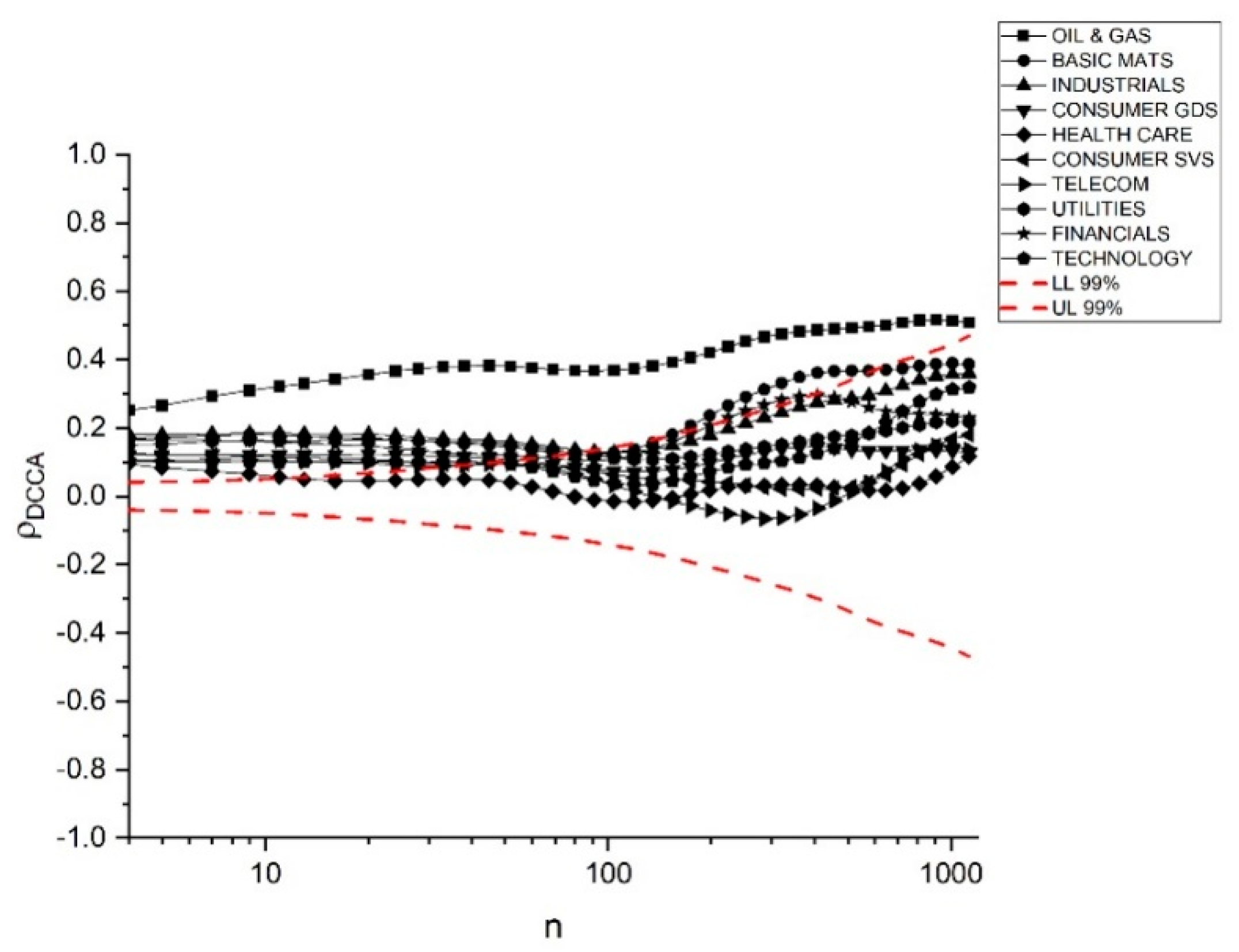
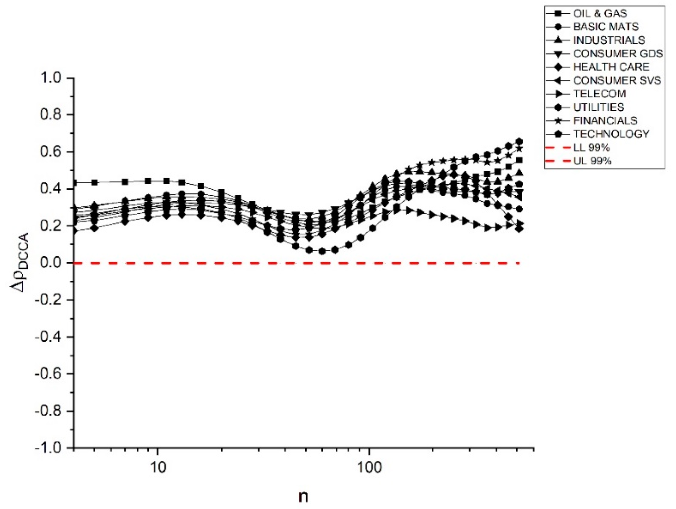
We proceeded to calculate the for the whole sample, with the results in Figure 1. As expected, the sector most closely related with WTI oil is the oil and gas index, with significant correlation coefficients regardless of the time scales analyzed. For the remainder, although with lower absolute levels, all the indexes show correlation with oil for lower time scales. In the case of medium time scales, basic materials and financials are the only indexes with some correlation with oil (although with marginal significance). For longer time scales, except for the correlation with the oil and gas sector, none of the other sectors correlates with oil.
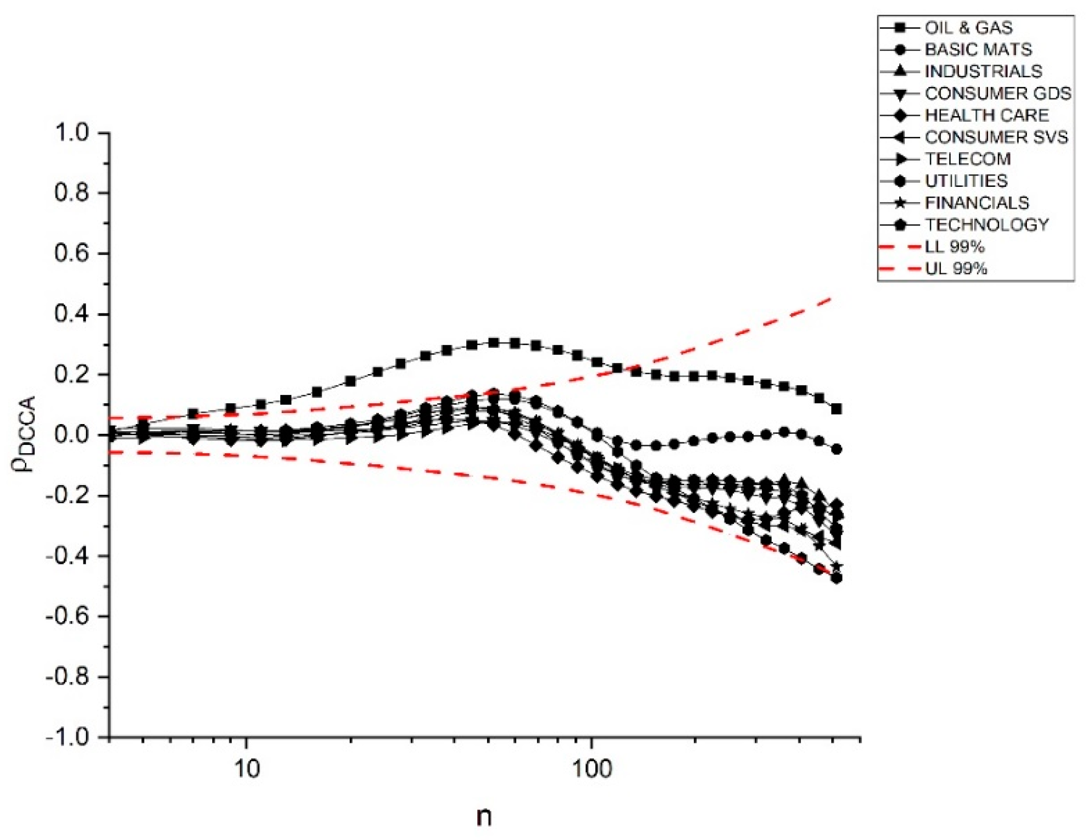
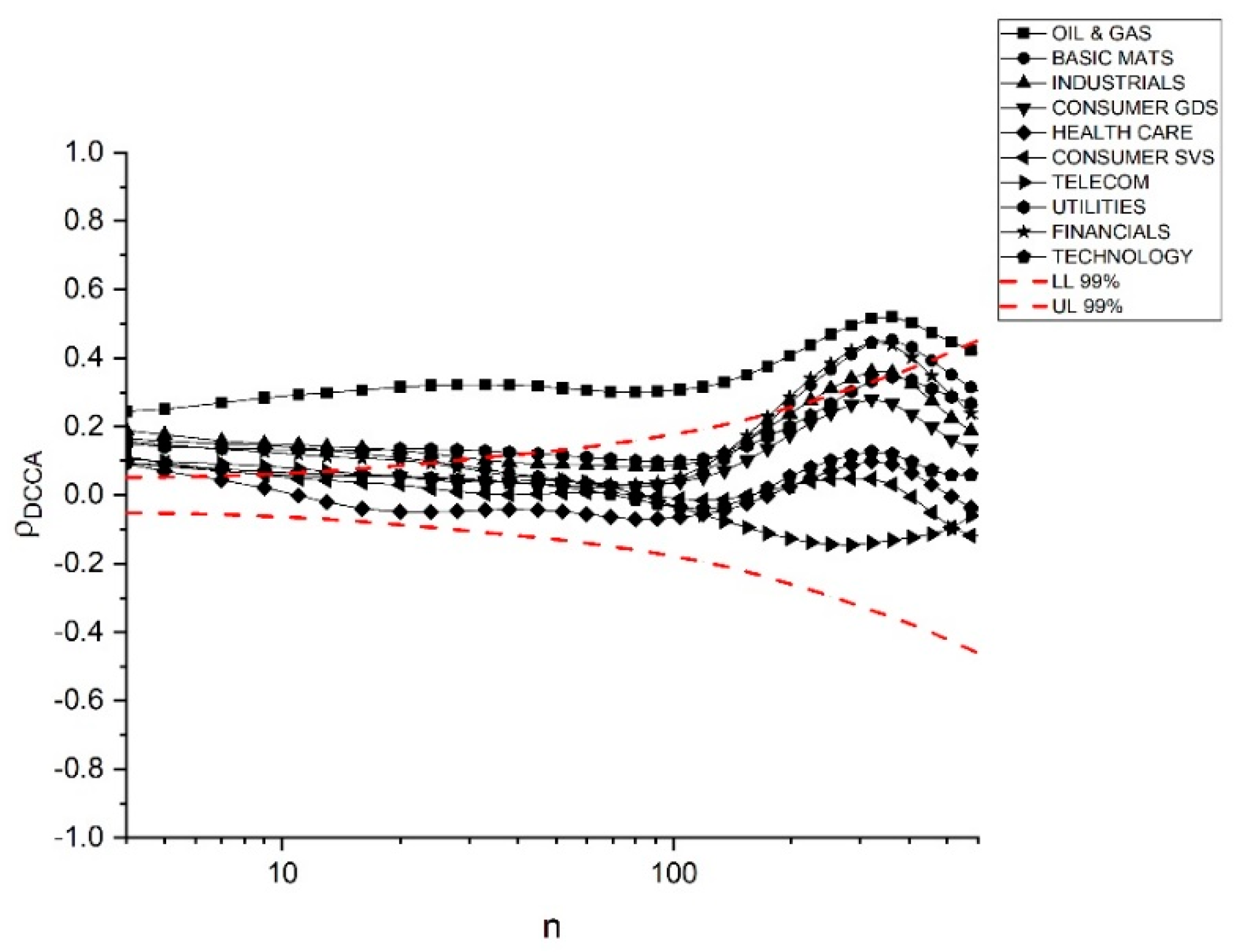
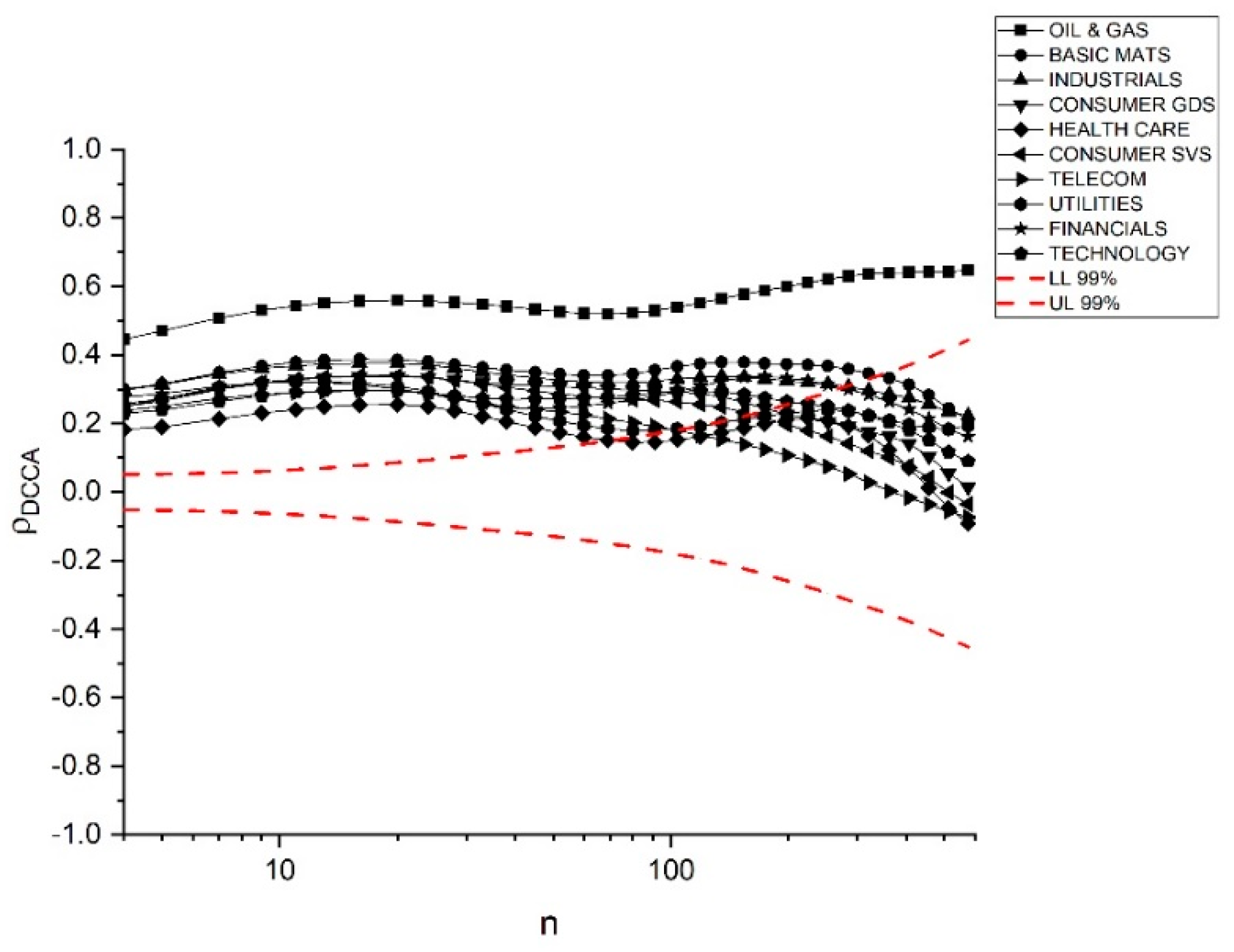
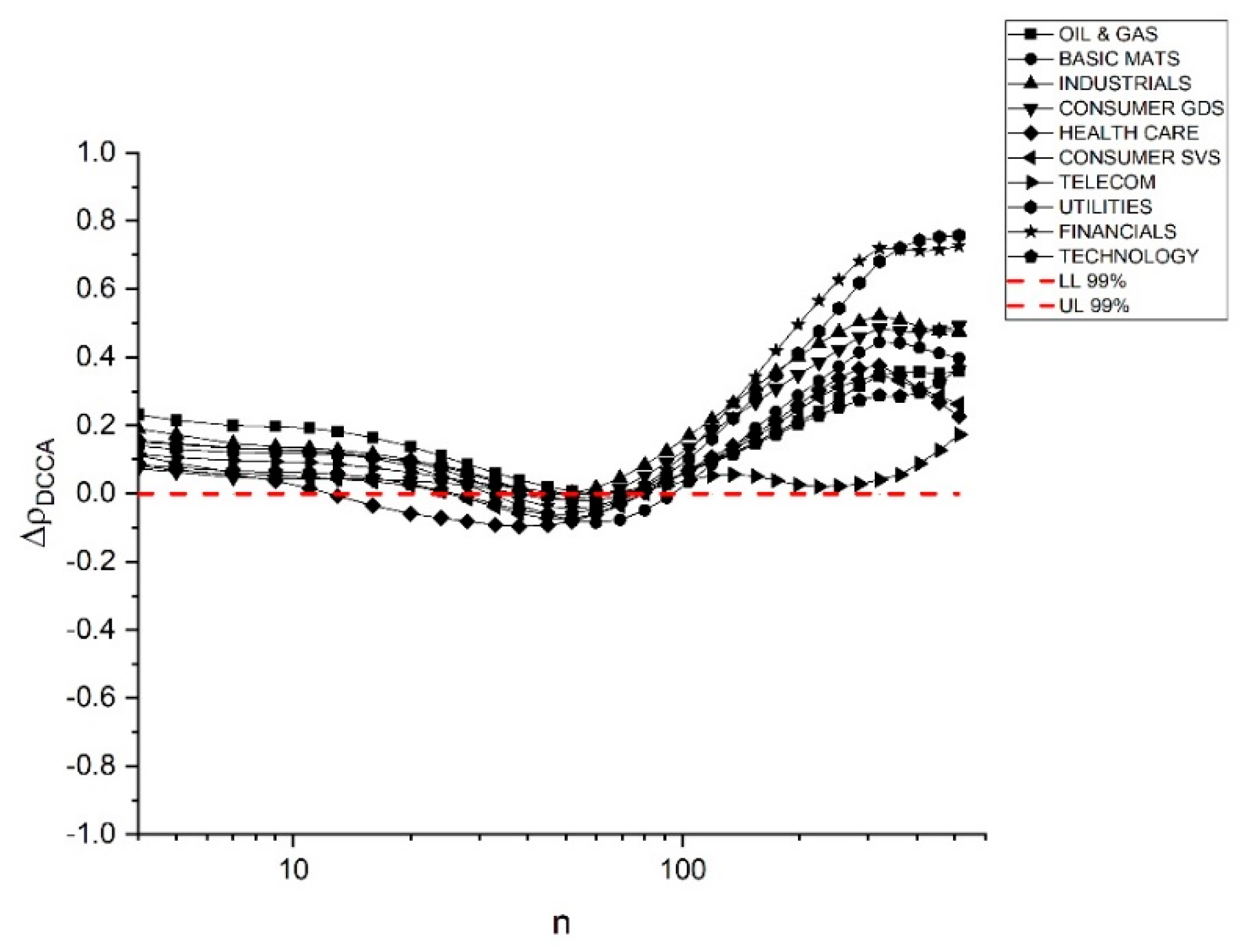
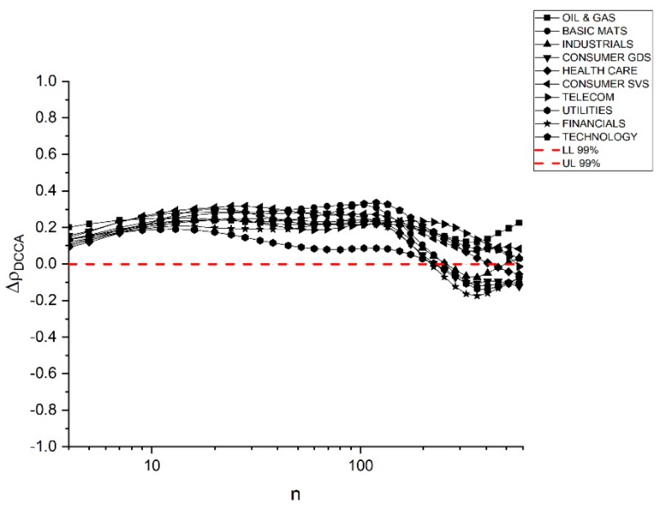
Correlations were calculated for the whole time sample. However, as we want to evaluate the evolution of correlations over time, we calculated the correlations for three different periods: the 1990s (results in Figure 2), the 2000s (Figure 3), and the 2010s (Figure 4).
During the 1990s (Figure 2), the oil and gas index was the only one with a significant correlation with WTI oil price, and just for scales from 7 to about 100 days. In the short run and in the long run, oil had no correlation with any industrial sector. The 1990s are remembered as the golden years of economic growth, with relatively low oil prices, which could explain these results. In other words, with sustainable economic growth, the different industrial indexes were influenced by variables other than the evolution of oil prices.
In the following decade, with the correlations represented in Figure 3, a positive and significant correlation of oil with the Oil and Gas sector is identified (only in the longer time scale is the correlation marginally non-significant). In the short run, most sectors are influenced by oil price, while in the long run, sectors like basic materials, financials and industrials are also influenced. In the case of basic materials and industrials, as oil could be used both as energy for those industries and in the production of raw materials, the correlation could be made in this indirect way. In the case of the financial sector, it could be explained by the introduction of oil price in different financial products made available by providers of financial services.
Finally, in the 2010s (Figure 4), the oil and gas sector has a positive and significant correlation with oil price movements, while all the other indexes have significant correlations for longer time scales compared to the past situation (although in the long run those correlations are not statistically significant).
The change in the pattern of correlations is quite evident, making it interesting to analyze the evolution of the over time. With this objective, we calculate the to evaluate that change, also employing the test proposed by [57,58], considering the critical values identified in Table 2 (see Appendix B for details of this test). Note that these critical values are close to zero, making it difficult to distinguish between negative and positive values, but allowing analysis of the statistical significance of the data. Note that for time scales higher than n = 250 we used the same critical values.
Considering the for the whole dataset, i.e., when (Figure 5), we can see that all sectors increased the correlations with oil price, with oil and gas showing some predominance for short time scales, but with utilities and financials also showing a sharp increase for longer time scales. Telecommunications and health care seem to be sectors with a low amount of changes in correlations over this period.
Regarding the difference between the first and second periods (, with results in Figure 6), in general we note an increase of the correlation pattern both in short and long time scales, with utilities and financials as the sectors changing most. Curiously, for middle short scales, the correlations decreased over both periods. Once again, telecommunications and health care show less changes.
Finally, for the last two periods under analysis (when ), the increase is more stable for the whole set of time scales. In the short run, all sectors correlated more with oil in the 2010s than in the 2000s. However, for scales over 100, the increase in correlations falls and in most cases negative values are found (Figure 7).
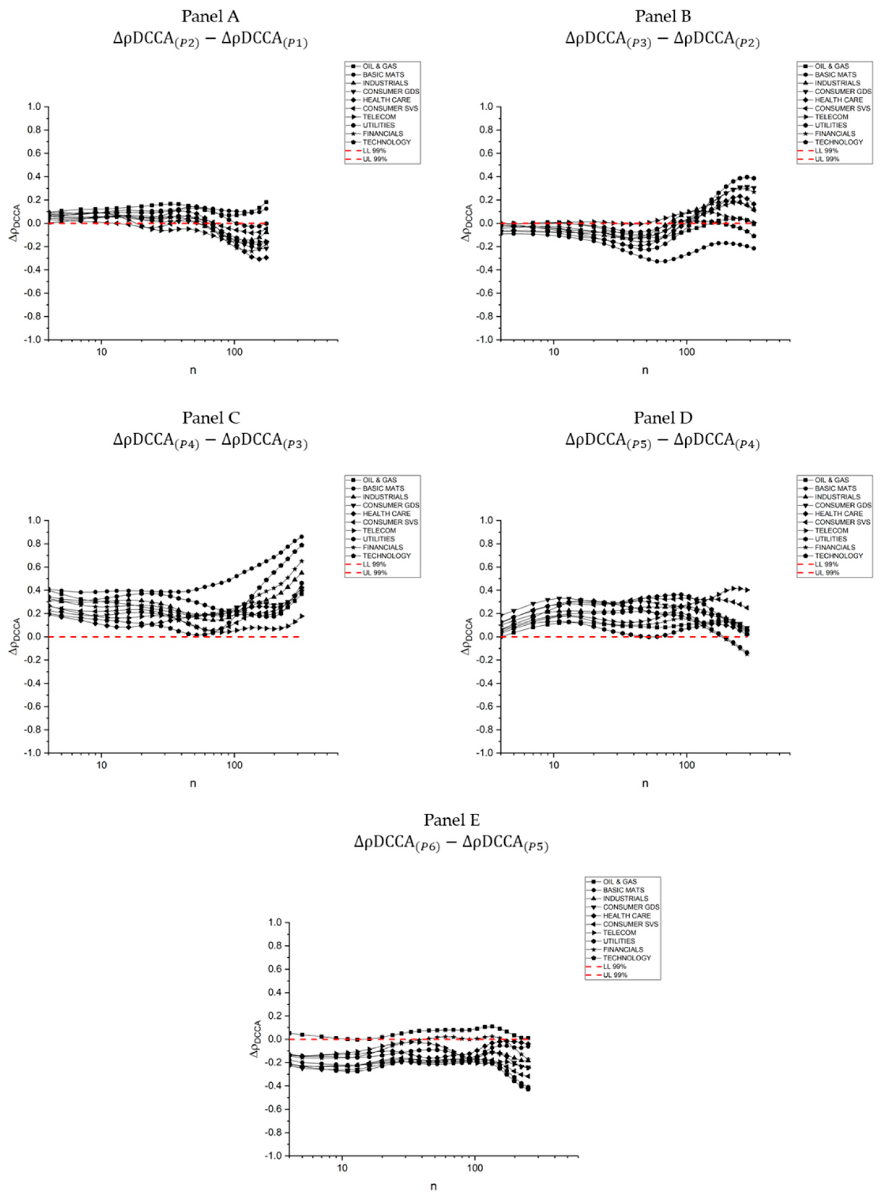
For a more detailed analysis of the evolution of the comovements studied, we made a similar analysis considering consecutive 5-year periods (see Table A1 of Appendix C for details of the different periods). The results, presented in Figure A1 of Appendix C, corroborate previous findings and show that the periods of higher increase of correlations were after the passing of the millennium. However, this subdivision reveals that since 2015, the correlation levels of most sectors decreased, correcting the increased exposure of the previous periods. In this last 5-year period, European stock markets recovered from the losses of the crisis, while the behavior of crude oil prices was more stable. Future research, extending the size of the sample, would be useful to understand the pattern of correlations.
5. Discussion and Policy Implications
In this study, we analyze how WTI oil is related to different industrial sector indexes provided by Euro Stoxx. Firstly, we are interested in understanding which indexes are the most affected by oil price fluctuation and secondly, whether (and how) those correlations changed over time.
As expected, the sector most closely related to oil is oil and gas, although in the 1990s the relationship was not statistically significant. For the remaining periods, the correlations are positive and have a tendency to increase. For the rest of the indexes, the 1990s and 2000s show low or no correlation with oil, although in the 2010s all the indexes showed significant correlations for short time scales and some of them show significant correlations for almost all time scales.
In fact, if we make the analysis with the , which shows the evolution of correlation over time, we can conclude that all the sector indexes are more related with oil now than in the past, with the highest increase seen in utilities, financials, oil and gas and industrials. Although the highest values of are between the 1990s and the 2000s, most of the indexes increased their correlations with oil in the 2010s, and this could be the most important conclusion.
Some of these results can be explained by the following: between 1990 and 2007, oil consumption and transport emissions increased by 36%, driven by increases in demand. Additionally, energy efficiency improvements in air and cargo transport have, until now, been limited. In 2013 alone, greenhouse gas emissions from transport were 13% above 1990 levels. Another point is that the EU’s dependence on crude oil imports is high and has increased over the past three decades. Imports now account for 88% of the EU’s oil supply [1].
Regarding the increased exposure in the particular case of the financial sector, one possible explanation is that portfolios of large banks, hedge funds and pension funds are composed of assets in sectors linked to fossil fuels and linked to the energy sector. In this context, in an analysis of European markets, [63] identified that aggregate exposures of investment funds, insurance and pension funds, banks, other credit institutions and other financial services were close to 32.4 trillion dollars, equivalent to 58.7% of total market capitalization, with a large part of these companies’ portfolios being composed of assets from companies related to the energy and fossil fuels sector. As a result, it is natural that major fluctuations in oil prices directly affect European financial institutions, since a large part of their capital is allocated to companies in the energy sector, especially those related to the oil sector.
Oil prices are inherently volatile, so major fluctuations can lead to uncertainty, reducing investor confidence and affecting economic growth. So, the increase in oil price that happened around 2008 raised inflation in the EU, mainly because of the impact on the cost of mobility, for which short-term price elasticities are typically low [1].
Moreover, most oil trade takes place on stock exchanges. Transactions take the form of hedging or speculative operations, based on more or less subjective predictions of the geopolitical, economic, energy and even meteorological contexts (harsh winters, hurricanes, etc.) Psychological factors can therefore also strongly influence price trends. In this context, hedging is practiced mainly by producers and consumers (refineries, airlines, etc.) who wish to minimize the risks associated with possible sudden price fluctuations when buying or selling oil, limiting their risks. Usually, speculation is practiced by operators who aim to make a profit by banking on market trends. Unlike hedging, speculation involves taking risks. Being practiced by non-specialists in the oil industry, speculation increases volatility, increasing the extent of price variations.
The increasing dependence of European stock markets on oil price over the past three decades has been detrimental to the European Union in several aspects: economic, geopolitical, financial and environmental. In this section, we will discuss these aspects and point out possible alternatives to reduce this dependency.
From an economic point of view, petroleum products accounted for about 38% of primary energy consumption in 2011 in the EU, with transport and petrochemical industries as the main indexes, accounting for about 80% of this consumption. In 2014, 88% of the crude oil consumed in the EU came from imports and this dependency is still increasing. In 2015, the total amount of EU crude oil imports was about 187 billion euros, about 1.3% of the EU’s GDP [1].
From a geopolitical point of view, it is crucial to understand that about 30% of EU crude oil imports came from Russia, 16% from Nigeria and sub-Saharan Africa, 16% from the Middle East and 8% from North Africa. So, EU imports are largely from politically unstable regions suffering from terrorism, internal conflicts or wars. This contributes to oil price volatility, which influences important EU sectors such as transport, medicine, food and petrochemicals [1].
As much of the world’s oil trading takes place on the stock exchanges, basically in the New York Mercantile Exchange (NYMEX) and in the New York and Atlanta-based Intercontinental Exchange (ICE), the price of oil is subject to variations according to the geopolitical (wars, conflicts, etc.), economic (subject to economic and exchange rate crises, etc.) and meteorological (severe winters, hurricanes, etc.) contexts, but also subject to hedging or speculation operations. Moreover, the price elasticity of essential goods tends to be low, and this also applies to oil. In other words, a big change in oil price could have a small impact on demand. So, greater dependence on oil prices implies that any possible shock could cause instability in several sectors of the European economy, as oil products are present in key sectors such as transport, medicines, food and petrochemicals, among others, where there are few alternatives [64]. Additionally, [63] found that the largest banks in the Eurozone have higher levels of direct and indirect exposure to sectors that could be affected by that dependence, with possible adverse systemic consequences if such a shock occurs.
In order to reduce its dependency, the EU has a plan to improve energy efficiency (by at least 27% by 2030), to decarbonize the economy (with a reduction target of 40% of emissions by 2040) and laws to limit cars’ emissions in 2021, besides promises of new post-2020 efficiency standards by the European Commission. To achieve these objectives, for example, EU vehicle manufacturers will have to make energy efficiency improvements in technologies and increase the share of low carbon vehicles (such as electric cars). Individually, some EU countries such as France, Austria and the Netherlands have already set an end date for the sale of diesel and petrol-powered cars (other European countries such as Norway have made similar decisions).
Whatever the future price of oil, it is clear that improvements in fuel efficiency and measures to reduce oil demand will improve the resilience of the EU economy to possible oil price shocks.
Investment in the production of biofuels could also be an alternative to reduce EU sectors’ dependence on oil. This kind of energy is seen as an excellent alternative because it is produced by renewable sources which can be produced regionally, helping to reduce dependence on oil from politically unstable regions and promoting environmental improvements. However, it is important to note that the production of biofuels is also a controversial issue, since this involves high levels of energy consumption and is usually based in intensive cultures, with higher levels of water consumption, which also has negative effects on the environment. Moreover, it is linked with the destruction of large forested areas, which also have environmental properties.
This means that in different countries the use of biofuels has different patterns. For example, in Brazil, around 45% of energy and 18% of fuel consumed are already renewable, while in the EU this represents only 4.5% of the energy matrix. The comparison between biofuels produced in Brazil and Europe takes into account production and energy efficiency and economic sustainability. The energy balance of sugarcane ethanol is 9.3, much higher than the 2.5 for rapeseed (the most widely used biomass in the EU) biodiesel in the EU. Another point is that ethanol productivity is approximately 7000 liters per hectare, while biodiesel from rapeseed yield is around 1320 liters per hectare [65]. At the same time, the costs of producing ethanol from sugarcane are much lower than those necessary to produce biodiesel from rapeseed oil. According to [65], the costs estimated from empirical analysis are about 0.56/0.58 USD per liter for Brazilian sugarcane ethanol versus 1.00 USD per liter for European rapeseed biodiesel.
In conclusion, the imposition of measures like those described above contribute to reducing the risk of oil price fluctuations, as the various sector indexes increasingly correlate with the price of crude oil. Therefore, any oil price fluctuations may lead to uncertainty and increase financial speculation in oil prices, including key sectors in the European economy such as finance, industry and telecommunications.
The use of extensions of the DCCA, such as the application of multifractal DCCA, can help us to identify different issues, namely the possibility of analyzing the effects of correlation, distinguishing between short- and long-term effects (see, for example, [66,67]). This kind of approach could allow a deeper analysis and will be considered in future research.
Author Contributions
Conceptualization, P.F., É.J.A.L.P. and H.B.B.P.; Data curation, P.F., É.J.A.L.P. and H.B.B.P.; Formal analysis, P.F., É.J.A.L.P. and H.B.B.P; Methodology, P.F., É.J.A.L.P. and H.B.B.P; Writing—original draft, P.F., É.J.A.L.P. and H.B.B.P; Writing—review and editing, P.F., É.J.A.L.P. and H.B.B.P. All authors have read and agreed to the published version of the manuscript.
Funding
Paulo Ferreira is pleased to acknowledge financial support from Fundação para a Ciência e a Tecnologia (grant UID/ECO/04007/2019).
Conflicts of Interest
The authors declare no conflict of interest.
Appendix A
In this appendix, we present the DFA methodology proposed by [44]. The steps are similar to those of DCCA, but considering just one time series, since DFA measures serial dependence. So, for a time with length N, first is the calculation , which consists of integrating the original one. The new time series is also divided in boxes of length n, for which we calculate the local trend, with OLS, obtaining , which is then used to detrend the time series and to obtain the fluctuation function of the DFA given by . Repeating this process for the different window sizes (n), regressing the log of F(n) and n allows us to obtain a power-law given by , with α representing the Hurst exponent, which measures the level of serial dependence, according to the following interpretations: if α = 0.5 the time series is a random walk, while if it is different from that value, the time series has some kind of dependence.
Appendix B
In this appendix, we explain the procedures of the test proposed by [51,52] to measure the difference in the DCCA correlation coefficient for two different periods. The authors built different time series, considering different lengths (from 250 to 2000 observations), based on ARFIMA (autoregressive integrated moving average) processes. Splitting the original time series in two parts, identifying a before and an after, these pairs were shuffled, allowing calculation of the for both parts (before and after) as well as the respective difference (). Repeating the process 10,000 times, the authors obtained the PDF function for , which was used to obtain the critical values presented in Table 2.
Appendix C
After the division of the whole sample in 10-year periods, we divided it in sequential 5-year periods, to analyze the evolution of the correlations over time for those shorter periods. Table A1 identifies the different periods and the results of the are presented in Figure A1.

Table A1.
Identification of the 5-year periods.
| Period | Years | Observations |
|---|---|---|
| P1 | 1992–1994 | 782 |
| P2 | 1995–1999 | 1305 |
| P3 | 2000–2004 | 1305 |
| P4 | 2005–2009 | 1304 |
| P5 | 2010–2014 | 1304 |
| P6 | 2015–2019 | 1117 |
Figure A1.
for the correlation between WTI oil and Euro Stoxx industrial indexes, considering sequential 5-year periods, as a function of n (days). Dashed lines are the critical values of the test developed by [57,58]. (A) measures ; (B) measures ; (C) measures ; (D) measures ; (E) measures . In this figure we can see that the periods of higher increase of correlations were after 2000. Since 2015 the correlation levels of most sectors decreased, correcting the increased exposure of the previous periods, associated to the recovery from the losses of the crisis, while the behavior of crude oil prices was more stable.

References
- Cambridge Econometrics. A Study on Oil Dependency in the EU. A Report for Transport and Environment; Cambridge Econometrics: Cambridge, UK, 2016; Available online: https://www.camecon.com/wp-content/uploads/2016/11/Study-on-EU-oil-dependency-v1.4_Final.pdf (accessed on 23 December 2019).
- Hamilton, J. Causes and Consequences of the Oil Shock of 2007-08; National Bureau of Economic Research: Cambridge, MA, USA, 2009; No. w15002. [Google Scholar]
- Hamilton, J. Historical Oil Shocks; National Bureau of Economic Research: Cambridge, MA, USA, 2011; No. w16790. [Google Scholar]
- Hamilton, J. Oil and the macroeconomy since World War II. J. Political Econ. 1983, 91, 228–248. [Google Scholar] [CrossRef]
- Gisser, M.; Goodwin, T. Crude oil and the macroeconomy: Tests of some popular notions: Note. J. Money Credit Bank. 1986, 18, 95–103. [Google Scholar] [CrossRef]
- Mork, K. Oil and the macroeconomy when prices go up and down: An extension of Hamilton’s results. J. Political Econ. 1989, 97, 740–744. [Google Scholar] [CrossRef]
- Hamilton, J. What is an oil shock? J. Econom. 2003, 113, 363–398. [Google Scholar] [CrossRef]
- Kilian, L.; Park, C. The impact of oil price shocks on the US stock market. Int. Econ. Rev. 2009, 50, 1267–1287. [Google Scholar] [CrossRef]
- Cerra, V. How can a strong currency or drop in oil prices raise inflation and the black-market premium? Econ. Model. 2019, 76, 1–13. [Google Scholar] [CrossRef]
- Ferreira, P.; Pereira, É.; Silva, M.; Pereira, H. Detrended correlation coefficients between oil and stock markets: The effect of the 2008 crisis. Physica A 2019, 517, 86–96. [Google Scholar] [CrossRef]
- Smyth, R.; Narayan, P.K. What do we know about oil prices and stock returns? Int. Rev. Financ. Anal. 2018, 57, 148–156. [Google Scholar] [CrossRef]
- Busch, T.; Bauer, R.; Orlitzky, M. Sustainable Development and Financial Markets: Old Paths and New Avenues’. Bus. Soc. 2015, 55, 303–329. [Google Scholar] [CrossRef]
- Amidu, M.; Issahaku, H. The role of financial markets in promoting sustainability—A review and research framework. In Research Handbook of Investing in the Triple Bottom Line; Boubaker, S., Cumming, D., Nguyen, D., Eds.; Edward Elgar Publishing: Cheltenham, UK, 2018; pp. 264–291. [Google Scholar]
- Kaul, G.; Seyhun, N. Relative price variability, real shocks, and the stock market. J. Financ. 1990, 45, 479–496. [Google Scholar] [CrossRef]
- Ferson, W.; Harvey, C. Predictability and time-varying risk in world equity markets. Res. Financ. 1995, 13, 25–88. [Google Scholar]
- Kaneko, T.; Lee, B. Relative importance of economic factors in the US and Japanese stock markets. J. Jpn. Int. Econ. 1995, 9, 290–307. [Google Scholar] [CrossRef]
- Jones, C.; Gautam, K. Oil and the stock markets. J. Financ. 1996, 51, 463–491. [Google Scholar] [CrossRef]
- Sadorsky, P. Oil price shocks and stock market activity. Energy Econ. 1999, 21, 449–469. [Google Scholar] [CrossRef]
- Hong, H.; Torous, W.; Valkanov, R. Do Industries Lead the Stock Market? Gradual Diffusion of Information and Cross-Asset Return Predictability; Working Paper; Stanford University: Stanford, CA, USA; UCLA: Los Angeles, CA, USA, 2002. [Google Scholar]
- Park, J.; Ratti, R. Oil price shocks and stock markets in the US and 13 European countries. Energy Econ. 2008, 30, 2587–2608. [Google Scholar] [CrossRef]
- Apergis, N.; Miller, S. Do structural oil-market shocks affect stock prices? Energy Econ. 2009, 31, 569–575. [Google Scholar] [CrossRef] [Green Version]
- Papapetrou, E. Oil price shocks, stock markets, economic activity and employment in Greece. Energy Econ. 2001, 23, 511–532. [Google Scholar] [CrossRef]
- Abhyankar, A.; Xu, B.; Wang, J. Oil price shocks and the stock market: Evidence from Japan. Energy J. 2013, 34, 199–222. [Google Scholar] [CrossRef]
- Moya-Martínez, P.; Ferrer-Lapeña, R.; Escribano-Sotos, F. Oil price risk in the Spanish stock market: An industry perspective. Econ. Model. 2014, 37, 280–290. [Google Scholar] [CrossRef]
- Filis, G.; Degiannakis, S.; Floros, C. Dynamic correlation between stock market and oil prices: The case of oil-importing and oil-exporting countries. Int. Rev. Financ. Anal. 2011, 20, 152–164. [Google Scholar] [CrossRef]
- Wang, Y.; Wu, C.; Yang, L. Oil price shocks and stock market activities: Evidence from oil-importing and oil-exporting countries. J. Comp. Econ. 2013, 41, 1220–1239. [Google Scholar] [CrossRef]
- Filis, G.; Chatziantoniou, I. Financial and monetary policy responses to oil price shocks: Evidence from oil-importing and oil-exporting countries. Rev. Quant. Financ. Account. 2014, 42, 709–729. [Google Scholar] [CrossRef] [Green Version]
- Huang, R.; Masulis, R.; Stoll, H. Energy shocks and financial markets. J. Futures Mark. 1996, 16, 1–27. [Google Scholar] [CrossRef]
- Hammoudeh, S.; Huimin, L. Oil sensitivity and systematic risk in oil-sensitive stock indices. J. Econ. Bus. 2005, 57, 1–21. [Google Scholar] [CrossRef]
- Sawyer, K.; Nandha, M. How Oil Moves Stock Prices; Working Paper Series; University of Melbourne: Melbourne, Australia, 2006. [Google Scholar]
- Faff, R.; Brailsford, T. Oil price risk and the Australian stock market. J. Energy Financ. Dev. 1999, 4, 69–87. [Google Scholar] [CrossRef]
- El-Sharif, I.; Brown, D.; Burton, B.; Nixon, B.; Russell, A. Evidence on the nature and extent of the relationship between oil and equity value in UK. Energy Econ. 2005, 27, 819–930. [Google Scholar] [CrossRef]
- Arouri, M.; Nguyen, D. Oil prices, stock markets and portfolio investment: Evidence from sector analysis in Europe over the last decade. Energy Policy 2010, 38, 4528–4539. [Google Scholar] [CrossRef] [Green Version]
- Arouri, M. Does crude oil move stock markets in Europe? A sector investigation. Econ. Model. 2011, 28, 1716–1725. [Google Scholar] [CrossRef]
- Scholtens, B.; Yurtsever, C. Oil price shocks and European industries. Energy Econ. 2012, 34, 1187–1195. [Google Scholar] [CrossRef]
- Degiannakis, S.; Filis, G.; Floros, C. Oil and stock returns: Evidence from European industrial sector indices in a time-varying environment. J. Int. Financ. Mark. Inst. Money 2013, 26, 175–191. [Google Scholar] [CrossRef] [Green Version]
- Badeeb, R.; Lean, H. Asymmetric impact of oil price on Islamic sectoral stocks. Energy Econ. 2018, 71, 128–139. [Google Scholar] [CrossRef]
- Gogineni, S. The Stock Market Reaction to Oil Price Changes; Working Paper; University of Oklahoma: Norman, OK, USA, 2007. [Google Scholar]
- Yurtsever, C.; Zahor, T. Oil Price Shocks and Stock Market in the Netherlands; Working Paper Series; University of Groningen: Groningen, The Netherlands, 2007. [Google Scholar]
- Nandha, M.; Faff, R. Does oil move equity prices? A global view. Energy Econ. 2008, 30, 986–997. [Google Scholar] [CrossRef]
- Zhang, D. Oil shock and economic growth in Japan: A nonlinear approach. Energy Econ. 2008, 30, 2374–2390. [Google Scholar] [CrossRef]
- Aloui, C.; Jammazi, R. The effects of crude oil shocks on stock market shifts behaviour: A regime switching approach. Energy Econ. 2009, 31, 789–799. [Google Scholar] [CrossRef]
- Zhang, D. Oil shocks and stock markets revisited: Measuring connectedness from a global perspective. Energy Econ. 2017, 62, 323–333. [Google Scholar] [CrossRef]
- Zebende, G. DCCA cross-correlation coefficient: Quantifying level of cross-correlation. Physica A 2011, 390, 614–618. [Google Scholar] [CrossRef]
- Podobnik, B.; Stanley, H. Detrended cross-correlation analysis: A new method for analysing two nonstationary time series. Phys. Rev. Lett. 2008, 100, 084102. [Google Scholar] [CrossRef] [Green Version]
- Peng, C.; Buldyrev, S.; Havlin, S.; Simons, M.; Stanley, H.; Goldberger, A. Mosaic organization of DNA nucleotides. Phys. Rev. E 1994, 49, 1685. [Google Scholar] [CrossRef] [Green Version]
- Vandewalle, N.; Ausloos, M. Coherent and random sequences in financial fluctuations. Physica A 1997, 246, 454–459. [Google Scholar] [CrossRef]
- Liu, Y.; Cizeau, P.; Meyer, M.; Peng, C.; Stanley, H. Correlations in economic time series. Physica A 1997, 245, 437–440. [Google Scholar] [CrossRef] [Green Version]
- Ausloos, M.; Vandewalle, N.; Boveroux, P.; Minguet, A.; Ivanova, K. Applications of statistical physics to economic and financial topics. Physica A 1999, 274, 229–240. [Google Scholar] [CrossRef]
- Ausloos, M. Statistical physics in foreign exchange currency and stock markets. Physica A 2000, 285, 48–65. [Google Scholar] [CrossRef]
- Podobnik, B.; Jiang, Z.; Zhou, W.; Stanley, H. Statistical tests for power-law cross-correlated processes. Phys. Rev. E 2011, 84, 066118. [Google Scholar] [CrossRef] [PubMed] [Green Version]
- Kristoufek, L. Measuring correlations between non-stationary series with DCCA coefficient. Physica A 2014, 402, 291–298. [Google Scholar] [CrossRef] [Green Version]
- Kristoufek, L. Detrending moving-average cross-correlation coefficient: Measuring cross-correlations between non-stationary series. Physica A 2014, 406, 169–175. [Google Scholar] [CrossRef] [Green Version]
- Wang, G.; Xie, C.; Chen, Y.; Chen, S. Statistical Properties of the Foreign Exchange Network at Different Time Scales: Evidence from Detrended Cross-Correlation Coefficient and Minimum Spanning Tree. Entropy 2013, 15, 1643–1662. [Google Scholar] [CrossRef]
- Zhao, X.; Shang, P.; Huang, J. Several fundamental properties of DCCA cross-correlation coefficient. Fractals 2017, 25, 1750017. [Google Scholar] [CrossRef]
- Silva, M.; Pereira, É.; Filho, A.; Castro, A.; Miranda, J.; Zebende, G. Quantifying the contagion effect of the 2008 financial crisis between the G7 countries (by GDP nominal). Physica A 2016, 453, 1–8. [Google Scholar] [CrossRef]
- Guedes, E.; Brito, A.; Filho, F.; Fernandez, B.; Castro, A.; Filho, A.; Zebende, G. Statistical test for ∆ρDCCA cross-correlation coefficient. Physica A 2018, 501, 134–140. [Google Scholar] [CrossRef]
- Guedes, E.; Brito, A.; Filho, F.; Fernandez, B.; Castro, A.; Filho, A.; Zebende, G. Statistical test for ∆ρDCCA: Methods and data. Data Brief 2018, 18, 795–798. [Google Scholar] [CrossRef]
- Ma, F.; Wei, Y.; Huang, D.; Zhao, L. Cross-correlations between West Texas Intermediate crude oil and the stock markets of the BRIC. Physica A 2013, 392, 5356–5368. [Google Scholar] [CrossRef]
- Ma, F.; Zhang, Q.; Peng, C.; Wei, Y. Multifractal detrended cross-correlation analysis of the oil-dependent economies: Evidence from the West Texas intermediate crude oil and the GCC stock markets. Physica A 2014, 410, 154–166. [Google Scholar] [CrossRef]
- Hussain, M.; Zebende, G.; Bashir, U.; Donghong, D. Oil price and exchange rate co-movements in Asian countries: Detrended cross-correlation approach. Physica A 2017, 465, 338–346. [Google Scholar] [CrossRef]
- Yang, L.; Zhu, Y.; Wang, Y.; Wang, Y. Multifractal detrended cross-correlations between crude oil market and Chinese ten sector stock markets. Physica A 2016, 462, 255–265. [Google Scholar] [CrossRef]
- Battiston, S.; Mandel, A.; Monasterolo, I.; Schütze, F.; Visentin, G. A climate stress-test of the financial system. Nat. Clim. Chang. 2017, 7, 283–288. [Google Scholar] [CrossRef]
- Helbing, D. Globally networked risks and how to respond. Nature 2013, 497, 51–59. [Google Scholar] [CrossRef]
- Shikida, P.; Finco, A.; Cardoso, B.; Galante, V.; Rahmeier, D.; Bentivoglio, D.; Rasetti, M. A comparison between ethanol and biodiesel production: The Brazilian and European experiences. In Liquid Biofuels: Emergence, Development and Prospects; Padula, D., Santos, M., Santos, O., Borenstein, D., Eds.; Springer: London, UK, 2014; pp. 25–53. [Google Scholar]
- Yuxin, C.; Yongping, R. Multifractal detrended cross-correlations between WTI crude oil price fluctuations and investor fear gauges. Appl. Econ. Lett. 2019, 26, 587–593. [Google Scholar]
- Shuping, L.; Xinheng, L.; Xinghua, L. Dynamic relationship between Chinese RMB exchange rate index and market anxiety: A new perspective based on MF-DCCA. Physica A 2020, 541, 123405. [Google Scholar]
Figure 1.
Detrended cross-correlation analysis coefficient (DCCA) correlation coefficient between WTI oil and each of the Euro Stoxx industrial indexes, for the whole time period, depending on n (time scales, in days). Dashed lines represent lower and upper critical values, for the test of hypotheses H0: and H1: .

Figure 2.
DCCA correlation coefficient between WTI oil and each of the Euro Stoxx industrial indexes, for the 1990s, depending on n (time scales, in days). Dashed lines represent lower and upper critical values, for the test of hypotheses H0: and H1: .
Figure 2.
DCCA correlation coefficient between WTI oil and each of the Euro Stoxx industrial indexes, for the 1990s, depending on n (time scales, in days). Dashed lines represent lower and upper critical values, for the test of hypotheses H0: and H1: .

Figure 3.
DCCA correlation coefficient between WTI oil and each of the Euro Stoxx industrial indexes, for the 2000s, depending on n (time scales, in days). Dashed lines represent lower and upper critical values, for the test of hypotheses H0: and H1: .
Figure 3.
DCCA correlation coefficient between WTI oil and each of the Euro Stoxx industrial indexes, for the 2000s, depending on n (time scales, in days). Dashed lines represent lower and upper critical values, for the test of hypotheses H0: and H1: .

Figure 4.
DCCA correlation coefficient between WTI oil and each of the Euro Stoxx industrial indexes, for the 2010s, depending on n (time scales, in days). Dashed lines represent lower and upper critical values, for the test of hypotheses H0: and H1: .
Figure 4.
DCCA correlation coefficient between WTI oil and each of the Euro Stoxx industrial indexes, for the 2010s, depending on n (time scales, in days). Dashed lines represent lower and upper critical values, for the test of hypotheses H0: and H1: .

Figure 5.
for the correlation between WTI oil and Euro Stoxx industrial indexes, for the whole period, as a function of n (days). Dashed lines are the critical values of the test developed by [57,58].

Figure 6.
for the correlation between WTI oil and Euro Stoxx industrial indexes, considering the 1990s–2000s period, as a function of n (days). Dashed lines are the critical values of the test developed by [57,58].

Figure 7.
for the correlation between WTI oil and Euro Stoxx industrial indexes, considering the 2000s–2019 period, as a function of n (days). Dashed lines are the critical values of the test developed by [57,58].

Table 1.
Descriptive statistics of the financial assets used.
| Index/Asset | Mean | Std. Dev. | Maximum | Minimum | Skewness | Kurtosis |
|---|---|---|---|---|---|---|
| Oil and gas | 0.0002 | 0.0141 | 0.1308 | −0.1012 | −0.0369 | 6.3815 |
| Basic mats | 0.0003 | 0.0134 | 0.1138 | −0.0865 | −0.1405 | 5.9745 |
| Industrials | 0.0003 | 0.0127 | 0.1105 | −0.1047 | −0.1915 | 7.0724 |
| Consumer goods | 0.0003 | 0.0124 | 0.2242 | −0.1538 | 0.6018 | 23.9259 |
| Health care | 0.0003 | 0.0126 | 0.0967 | −0.0871 | −0.1139 | 4.0665 |
| Consumer services | 0.0002 | 0.0114 | 0.0859 | −0.0784 | −0.1981 | 4.8316 |
| Telecom | 0.0002 | 0.0151 | 0.1047 | −0.1456 | −0.0531 | 4.6648 |
| Utilities | 0.0002 | 0.0121 | 0.1567 | −0.0900 | −0.0132 | 9.3169 |
| Financials | 0.0001 | 0.0155 | 0.1536 | −0.1471 | −0.0387 | 8.4805 |
| Technology | 0.0002 | 0.0176 | 0.1122 | −0.1402 | −0.2021 | 5.1350 |
| Crude oil-West Texas Intermediate (WTI) | 0.0002 | 0.0229 | 0.1641 | −0.1709 | −0.1359 | 4.9830 |
Table 2.
Critical values to test the significance of (n), considering the confidence levels (CL) of 90%, 95% and 99% and N = 2000 [57,58].
| n = 4 | n = 8 | n = 16 | n = 32 | n = 62 | n = 125 | n = 250 | |
|---|---|---|---|---|---|---|---|
| CL = 90% | 0.0009 | 0.0008 | 0.0008 | 0.0008 | 0.0008 | 0.0008 | 0.0008 |
| CL = 95% | 0.0010 | 0.0010 | 0.0009 | 0.0009 | 0.0009 | 0.0009 | 0.0010 |
| CL = 99% | 0.0014 | 0.0013 | 0.0012 | 0.0012 | 0.0012 | 0.0012 | 0.0013 |
© 2020 by the authors. Licensee MDPI, Basel, Switzerland. This article is an open access article distributed under the terms and conditions of the Creative Commons Attribution (CC BY) license (http://creativecommons.org/licenses/by/4.0/).
Share and Cite
MDPI and ACS Style
Ferreira, P.; Pereira, É.J.A.L.; Pereira, H.B.B. The Exposure of European Union Productive Sectors to Oil Price Changes. Sustainability 2020, 12, 1620. https://0-doi-org.brum.beds.ac.uk/10.3390/su12041620
AMA Style
Ferreira P, Pereira ÉJAL, Pereira HBB. The Exposure of European Union Productive Sectors to Oil Price Changes. Sustainability. 2020; 12(4):1620. https://0-doi-org.brum.beds.ac.uk/10.3390/su12041620
Chicago/Turabian StyleFerreira, Paulo, Éder J. A. L. Pereira, and Hernane B. B. Pereira. 2020. "The Exposure of European Union Productive Sectors to Oil Price Changes" Sustainability 12, no. 4: 1620. https://0-doi-org.brum.beds.ac.uk/10.3390/su12041620
Note that from the first issue of 2016, this journal uses article numbers instead of page numbers. See further details here.