Public Environment Emotion Prediction Model Using LSTM Network


1
College of Computer Science and Engineering, Northwest Normal University, Lanzhou 730070, Gansu Province, China
2
College of Mathematics and Statistics, Northwest Normal University, Lanzhou 730070, Gansu Province, China
*
Author to whom correspondence should be addressed.
Sustainability 2020, 12(4), 1665; https://0-doi-org.brum.beds.ac.uk/10.3390/su12041665
Submission received: 19 January 2020
/
Revised: 14 February 2020
/
Accepted: 19 February 2020
/
Published: 23 February 2020
(This article belongs to the Section Psychology of Sustainability and Sustainable Development)
Abstract
:Public environmental sentiment has always played an important role in public social sentiment and has a certain degree of influence. Adopting a reasonable and effective public environmental sentiment prediction method for the government’s public attention in environmental management, promulgation of local policies, and hosting characteristics activities has important guiding significance. By using VAR (vector autoregressive), the public environmental sentiment level prediction is regarded as a time series prediction problem. This paper studies the development of a mobile “impression ecology” platform to collect time spans in five cities in Lanzhou for one year. In addition, a parameter optimization algorithm, WOA (Whale Optimization Algorithm), is introduced on the basis of the prediction method. It is expected to predict the public environmental sentiment more accurately while predicting the atmospheric environment. This paper compares the decision performance of LSTM (Long Short-Term Memory) and RNN (Recurrent Neural Network) models on the public environment emotional level through experiments, and uses a variety of error assessment methods to quantitatively analyze the prediction results, verifying the LSTM’s performance in prediction performance and level decision-making effectiveness and robustness.
1. Introduction
The atmospheric environment is the natural space in which human beings live, and it is also the physical space in which human production and life directly interact [1]. While the atmospheric environment has improved in recent years, its real situation still worries us [2,3,4,5]. While resolving this kind of problem, we also found that the “environmental panic” [6] problem caused by the atmospheric pollution problem is becoming more and more serious [7,8,9]. For example, when there is smog, the public shows a negative attitude towards work and life and reduces going out. The public has different “emotions” to the environment because of various “situations” of the environment. This environmental mood is formed by public subjective consciousness and interferes with our thinking and behaviors [10]. It can also affect our social emotions. However, the implementation of some government policies and the organization of events have not received the expected good results due to the impact of public environmental sentiments [11,12,13,14,15]. Therefore, public environmental sentiment prediction is of great significance. This article will carry out a deep research over whether the public environmental emotion can be predicted, and how we should capture and collect the public environmental emotion [16]. Can public environmental sentiments be predicted? If they can be predicted, how will we predict them? In the study of this paper, we put forward the hypothesis that we believe that the relationship between atmospheric environmental factors and public environmental emotions can be used to predict the public environmental emotions. Then, what is the relationship between public environmental emotions and atmospheric environment? Yu Guoming, Professor of Beijing Normal University, said that the quality of the atmospheric environment affects the normal life and work of the public all the time. It is an important proposition related to social stability to study the impact of the atmospheric environment on the public emotion [17,18,19,20]. Many studies are also trying to prove the relationship between weather and human emotions. Most of them use questionnaires, telephone access, public datasets or crawling micro blog data to obtain public environmental emotions [21]. For example, in 2006–2007, taking the information release of world earth day as an example, the survey information of the public’s perception of the ecological environment shows that everyone is basically in an ecological environment prone to negative emotions [22]; for example, Li Junzhi and others take Xi’an city and Shanghai city as an example, using micro blog big data to carry out the method of emotional analysis and correlation analysis, to carry out a comparative analysis of residents’ emotional data and air quality data in the two cities [23]. In summary, we believe that the atmospheric environment is related to the public’s emotions, and we can use atmospheric environmental factors to predict the public’s environmental emotions. However, from the perspective of data acquisition, there are obvious deficiencies in the way of obtaining public environmental emotions compared with the way of public participatory perception [24,25,26,27,28]. For example, in the way of questionnaire surveys and telephone interviews, the respondents often fail to fully reflect the time of the survey due to time constraints and subjective guidance factors of the investigators, which often results in the collection of data samples without great randomness and this has a great impact on the results [29]. For the way of crawling microblog data, the data is generally collected by searching for topics. The data is often user comments [30,31,32]. When studying the environment and public environmental emotions, it is necessary to quantify these microblog data and use the quantified microblog data for correlation analysis [33]. However, there are also microblog comments that are not only published for environmental factors. Comments are quantified to have a greater impact on the results.
Most of the existing domestic and international research on the prediction of environmental factors predict some factors of air quality itself. For example, Huang Jie and others adopted the stacking integration strategy to integrate RNN (Recurrent Neural Network) and CNN (Convolutional Neural Network), and put forward the RNN-CNN integrated deep learning prediction model, aiming at the air quality of 1466 monitoring stations in mainland China in 2016. Data are samples of instance validation [30]. Another example is Li Dong et al. In order to solve the problem of low precision in PM2.5 concentration prediction, this paper proposes an online PM2.5 daily concentration hybrid prediction model based on correlation analysis, autoregressive distribution lag model, Drosophila optimization algorithm and nuclear limit learning machine, and applies the model to five cities in the Guanzhong region, and verifies the model with the monitoring data from January 2016 to May 2017 [34]. Another example is Mahajan sachit et al. who developed a prediction method, which uses exponential smoothing with drift and real-time PM2.5 data obtained from large-scale deployment of Internet of things devices in Taichung, Taiwan, for experiment and evaluation. These studies tend to improve the existing prediction model for application research, and the influencing factors of application research are mostly used: PM2.5, PM10 [35]. However, how to learn and analyze the public’s cognition, understanding and behavior characteristics of environmental change through the data of atmospheric environmental factors, to guide the formulation of environmental management policies, to form correct environmental awareness and environmental public opinion, is the starting point and foothold of public environmental behavior, so it is of far-reaching significance to predict public environmental emotion through the existing environmental data.
This paper focuses on the study of the relationship between atmospheric environment and public environmental emotion and the application of the public environmental emotion prediction model. First of all, using the atmospheric environment data and public environmental sentiment data on time series, and using the vector autoregressive model (VAR) to analyze the influencing factors of “public environmental perception satisfaction”, the result is one or more influencing factors, which paves the way for the construction of a public environmental sentiment prediction model. In this paper, the LSTM neural network model and RNN neural network model will be used to predict the public environmental sentiment, and the “public environmental sentiment prediction model” will be determined by referring to the prediction accuracy and error analysis between the two models.
2. Materials and Methods
2.1. Data Materials
In the era of big data, the emergence of pervasive computing has greatly enriched and enhanced researchers’ access to data and ability. Social perception computing is the product of the integration of social computing and pervasive computing, which is driven by the demand of social computing and the development of pervasive computing technology. Social perception computing can obtain large-scale, objective, real-time and continuous information about human social behaviors and interactions through large-scale and multiple kinds of sensing devices, such as universal sensors (RFID, motion sensors, audio and video sensors, etc.), smart phones (GPS, call records, SMS), combined with email, web (DBLP, forums, social networking sites, blogs, wikis), etc. The continuous and dynamic field data provide a solid foundation for the study of human behavior understanding and interaction rule understanding. In addition to analysis and understanding, social perception computing also emphasizes providing intelligent assistance and support for human behavior and interaction from three levels: Individual, group and society.
The public’s perception and understanding of the change of regional ecological environment will directly determine the public’s satisfaction with the quality of the ecological environment, the enthusiasm to participate in environmental protection, environmental behavior and environmental awareness, and make a positive response to the government’s environmental management policies. Group intelligence perception is based on the perception mode of a human based perception unit (device), which forms a perception network through people’s existing mobile devices, and publishes the perception task to individuals or groups in the network to complete, so as to help professionals or the public to collect data, analyze information and share knowledge. Compared with the general way of perception, a large number of sensors need to be arranged in advance. Swarm intelligence perception uses the idea of crowdsourcing to assign tasks to the public with mobile devices, and the public upload their own perception data of mobile device use, playing the role of sensors, thus saving a large amount of costs. Swarm intelligence sensing has many advantages, such as flexible deployment, heterogeneous multi-source sensing data, wide and uniform coverage, high expansion and multi-function. It provides a new mode of sensing environment, collecting data and providing information services for data sensing, and has been focused on in the aspect of ecological environment sensing.
2.1.1. Data Sources of Public Environment Emotion
This paper studies the early development of the data service platform “impression ecology” app. In the early stage of project development, the platform data collection mechanism and data collection mode are designed, and the relevant researchers of environmental science and environmental psychology are contacted for cooperation and exchange. In the early stage of public environmental sentiment data, the user’s direct scoring mode is adopted. However, considering that this mode will influence or interfere with the intuitive environmental factors due to the user’s objective factors (such as gender, age, physical health, nature of work, etc.), another scheme design of data collection will be carried out.
After a comprehensive consideration of the above issues, this study decided to develop a calculation model, through which to calculate and quantify the public environmental sentiment of platform users. First of all, in the early stage of model design, researchers of environmental science and environmental psychology discussed the design of environmental perception words for the platform. These perception words refer to the human body’s intuitive feeling (vision, smell, touch, hearing, collective sense), as well as the systematic study of “body cognition”, and a total of 27 perception words were designed, shown as Table 1. After the design of perception words, the platform test stage is carried out, and the environment-friendly volunteers are recruited for the perception calculation model to collect the early data (in this part, only through the “impression ecology” platform, volunteers are required to select the perception words and score the environment at that time). The time span of the test stage is one year. The platform collected environmental perception data of volunteers, including perception words and scoring data of different environmental conditions in four seasons, which is called “public environmental satisfaction”. The data are shown in Table 2. In this paper, we use these experimental data to construct the “perception model” with the idea of multi model fusion. The test results show that the accuracy of the public environmental satisfaction calculated by the calculation model is high; the research can add the calculation model to the platform to collect the data of “public environmental satisfaction” for the study of public environmental sentiment prediction.
In Table 1, the value range of SATISFACTION is 0–100. We will subdivide this value later and divide it into different levels of public environmental sentiment. LABEL is the perceived word of design. Its main function is to calculate public environmental perception satisfaction. The “impression ecology” app was officially launched and operated for one year. Through the platform, thousands of users in Lanzhou collected “public environmental satisfaction” data, with a total of 35,505 time series data, covering the period from 1 October 2016 to 30 September 2017. According to the comprehensive analysis, there are different ages, genders, education levels and occupations among the users who submit the data. This study considers that the data is representative, and can be used to divide the emotional level of “public environmental satisfaction” and generate the public environmental emotional data needed by this study.
2.1.2. Level of Public Environment Emotion
In this study, after obtaining “public environmental satisfaction”, the next work will grade the satisfaction with reference to the AQI index (currently widely used in the international air environment quality assessment system). This study intends to divide “public environmental satisfaction” into six grades. First of all, we grade “public environmental satisfaction” without considering the time factor when we use the preliminary experimental data. Secondly, the user’s “satisfaction” score is used to measure the tendency degree of environmental emotions. The Wilson interval method is used to grade, and Bayesian average method is used to modify the grade.
The Wilson’s interval method is used to divide the level of environmental emotion. The calculation method is based on binomial distribution. The results are related to the environmental emotion tendency at all levels and the frequency of each emotion tendency. At the beginning of the hypothesis, there are only two options of “feeling good” and “feeling bad” to make it conform to binomial distribution, and according to the confidence level, the result is obtained, and is shown in Formula (1).
where Smax is the maximum score, pmin is the lower limit of Wilson interval, p is the favorable rate (usually the average value/total score), n is the total number of evaluations, K is the statistics constant (representing the statistics of Z at a certain confidence level).
In the modification of the Wilson interval method, the Bayesian average method is used. Strictly speaking, it is not a scoring model, but a balance model. Its core idea is to provide a compensation value so that it will not produce an unreliable rating due to a small number of scores, but reduce the proportion of the compensation value under a large number of scoring data, and finally make the public environmental sentiment rating more accurate and reliable with the increase of the “public environmental perception satisfaction”. The level results are shown in Table 3. The key codes (shown as Table 4) to achieve the classification of public environmental emotions are as follows:
2.1.3. Sources of Atmospheric Environment Data
The atmospheric environment data in this study corresponds to the public environmental sentiment data in time series and has the same time span, with a total of 35,505. The air pollutants in the air environment data include six main pollutant indexes (PM2.5, PM10, SO2, NO2, O3, CO), which are from the hourly air pollutant concentration data of five state-controlled city stations in Lanzhou, while the meteorological data (temperature, humidity, pressure, wind speed) are from China Weather Network, which collects the hourly meteorological data of five major urban areas in Lanzhou; this is shown in Table 5. The data source of atmospheric environment is real and reliable, but a small part of the data is missing. Considering that the difference between the data before and after the data collection is not big, this paper uses hot deck imputation to supplement the missing data nearby.
2.2. Methods of VAR and LSTM, RNN
The vector autoregression (VAR) model is established to analyze the relationship between public environmental sentiment and atmospheric environment. The VAR model is extended from the AR model. The VAR model is compared with the traditional econometric method. It can be found that the basis of this model is not economic theory, but a form of multi-party alliance. According to the characteristics of the atmospheric environment in Lanzhou City, the following factors are selected: PM2.5, PM10, temperature (TMP), humidity (HUM) as the indicators of public environmental sentiment.
The LSTM network solves the problem that RNN will produce a gradient explosion when processing long time series prediction. This is mainly because each neuron of the LSTM network adds a memory unit to judge whether the information is useful or not, which is suitable for processing and predicting important events with relatively long intervals and delays in time series. Three control gates are placed in the memory unit of LSTM; they are called input gate, forgetting gate and output gate. When a message enters the network of LSTM, it can be judged whether it is useful according to the rules. Only the information conforming to the algorithm authentication will be left, and the inconsistent information will be forgotten through the forgetting gate.
2.2.1. Construction of VAR Model
The VAR model can be used to predict the interconnected time series system, and also to analyze the dynamic impact of some random disturbances on variable systems, and then explain the impact of these disturbances on economic variables. The VAR model is shown in Formula (2):
where is k-dimensional endogenous variable; is coefficient matrix to be estimated; the independent and identical distribution is subject to expectation 0 and variance (where variance is covariance matrix of k-dimensional vector) , which can be correlated in the same period, but usually not with its own lag value or the variable on the right side of the equation; p is lag term.
2.2.2. VAR Model Calculation Process
In order to ensure the validity of the VAR model, the ADF test (unit root test) is used to test the data stability and it can be proven that the existence of the unit root process in the sequence is not stable, which will cause false regression in the regression analysis. The ADF tests whether there are unit roots in the time series studied. If there is a unit root in the time series, it indicates that the time series is not a stationary one; if there is no unit root in the time series, it indicates that the time series is a stationary one. Once the time series is non-stationary, but insists on using the VAR analysis method, it will affect the effectiveness of the analysis results. Take lnSatisfaction, lnPM2.5, lnPM10, lnTMP and lnHUM as test variables to conduct the stability test, so as to judge whether each time series is a stable variable. The test results are shown in Table 6.
It can be seen from Table 2 that the ADF of time series of lnSatisfaction, lnPM2.5, lnPM10, lnTMP and lnHUM at 5% and 10% significant levels are all lower than the critical value; that is to say, all pass the test and are stable time series, which can be modeled by vector autoregression model.
In order to ensure that the residual sequence obeys the white noise, the optimal lag period is determined by the Schwartz criterion (AIC) and the (AC) information minimum criterion. The lag period judgment results of the VAR model are shown in Table 7.
Furthermore, AR characteristic polynomials are used for the stability test. According to the optimal lag number of 4, the AR inverse root graph of the VAR (4) model stability test is obtained (as shown in Figure 1). It can be seen from Figure 1 that the inverse roots of AR characteristic polynomials are all in the unit circle. In the long run, the system model formed between public environmental satisfaction and other factors is stable, which indicates that the VAR (4) model can be used for subsequent research.
It can be seen from Table 2 that the optimal lag period of LR, FPE, AIC and HQ is 4, but the lag period of one index with the minimum value is different from other indexes; that is, the optimal lag period of the SC index is 3. Considering the validity of the VAR model and the integrity of information, the optimal lag time of the VAR model is determined to be 4, and VAR (4) is finally established.
2.2.3. LSTM (Long Short-Term Memory) Model Construction
Long and short-term memory networks—often referred to as “LSTM”—are special RNNs that can learn long-term patterns. They were first proposed by Hochreiter and schmidhuber (1997), and were refined and promoted by many people in later work. They are very well used in all kinds of problems and are now widely used
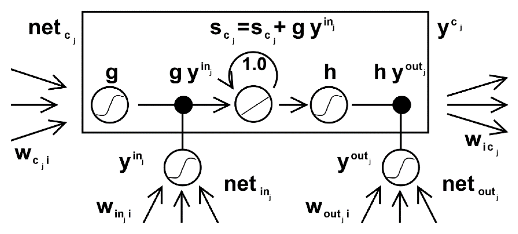
Long term short-term memory networks (LSTM) are extensions of recurrent neural networks, which basically extend their memory. Therefore, it is very suitable to learn from the important experience with a long time lag. The unit of LSTM is used as the building unit of the RNN layer, which is usually called the LSTM network. LSTM enables RNN to remember their input for a long time. This is because the LSTM includes their information in memory, much like the memory of a computer, because the LSTM can read, write, and delete information from memory. This memory can be regarded as a gating unit, which means that the unit decides whether to store or delete information (for example, whether it opens the door), which depends on the importance it gives information. The assignment of importance occurs in the weight, which is also learned by the algorithm. This simply means that it learns which information is important and which is not over time. The structure of LSTM neurons is shown in Figure 2.
The gates in LSTM are analog, in the form of S-shaped, meaning they range from 0 to 1, and being analog also allows them to propagate backwards. The problem of vanishing gradient can be solved by LSTM because it can keep the gradient steep enough, so the training is relatively short and the accuracy is high. The network structure of LSTM is shown in Figure 3.
Compared with the traditional cyclic neural network, LSTM is still based on xt and ht−1 to calculate ht, but the internal structure is designed more carefully. Three gates, i.e., input gate it, forgetting gate ft, output gate σt, and an internal memory unit ct are added. The input gate controls how much the new state of the current calculation is updated to the memory unit; the forgetting gate controls how much the information in the previous memory unit is forgotten; the output gate controls how much the current output depends on the current memory unit. In the classical LSTM model, the updated calculation is Formulas (3)–(6) of the t layer.
The calculation formula of the input door is shown in Formula (3):
The calculation formula of the forgetting gate is shown in Formula (4):
The calculation formula of the output gate is shown in Formula (5):
The calculation formula of the candidate layer is shown in Formula (6):
In a trained network, when there is no important information in the input sequence, the value of the forgetting gate of LSTM is close to 1, and the value of the input gate is close to 0. At this time, the past memory will be saved, so as to realize the long-term memory function. When there is important information in the input sequence, LSTM should store it in memory, and the value of the input gate will be close to 1. When the previous memory is no longer important, the value of the input gate is close to 1, and the value of the forgetting gate is close to 0, so the old memory is forgotten and the new important information is remembered. After such a design, the whole network more easily learns the long-term dependence between sequences.
2.2.4. RNN (Recurrent Neural Network) Model Construction
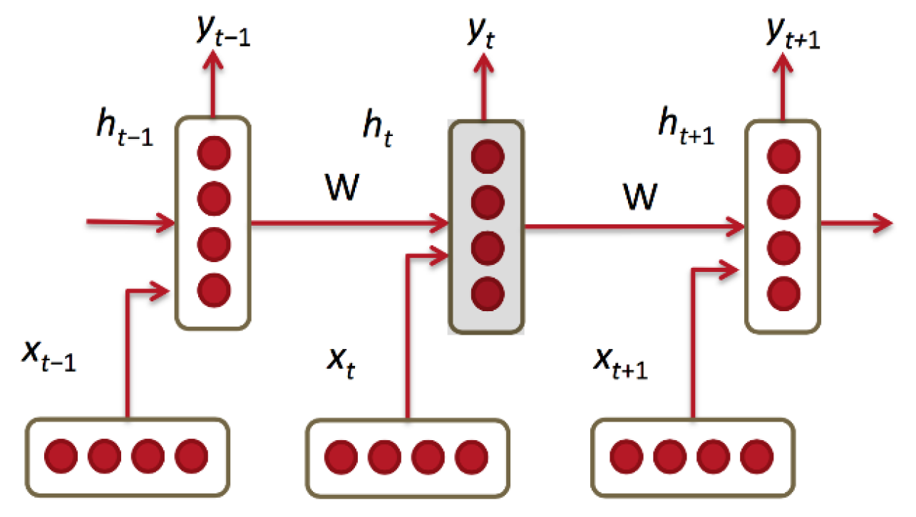
The training sample data in the CNN network is IID data (independent and identically distributed data), and the problem to be solved is also a classification problem, a regression problem, or a feature expression problem. However, more data does not meet IID, such as language translation and automatic text generation. They are a sequence problem, including time series and space series. At this time, the RNN network is used. The structure of the RNN is shown in Figure 4. RNN can not only process sequence input, but also get sequence output. The sequence here refers to the sequence of vectors. RNN learns a program; it can also be said to be a state machine, not a function. Taking sequence prediction as an example, the RNN network is introduced below:
- (1)
- The input is a time-varying vector sequence xt−2, xt−1, xt, xt+1, xt+2.
- (2)
- Estimated by model at time t as Formula (7):
- (3)
- It needs to take the current x as input and the previous hidden layer as input to get the output y.
2.2.5. Whale Optimization Algorithm (WOA)
In the behavior of whale hunting, we can see that it uses the strategy of contracting and encircling and spiraling. In order to simulate the behavior of this colleague, we refer to p. When the value of p is greater than 0.5, the spiral formula strategy is used. When p is less than 0.5, the formula strategy of encircling prey is used. In the process of encircling the sidetracking, it is necessary to judge whether the absolute value of vector a is greater than 1 to determine whether the current optimal solution is the one with the minimum use value or the current optimal solution of randomly selecting a seat. It can update the number of iterations plus the location of each search agent so as to constantly update the position of whales, and then calculate the fitness value of each whale according to the time when the whales to be searched are all updated once, and then select the whale with the smallest fitness value as the current “best result” and then update each iteration with different formulas by randomly generating the value of p until the number of iterations is satisfied.
Humpback whales can identify and surround prey. Since the position of the optimal design in the search speed is not known a priori, the WOA algorithm assumes that the current optimal candidate solution is the target prey or close to the optimal solution. After the best search agent is defined, other search agents attempt to update their location to the best search agent. This behavior is represented by Formulas (7) and (8):
where t represents the current iteration, A and C are the coefficient vectors, X* is the position vector of the best solution obtained at present, the X vector is the position vector. It is worth mentioning here that if there is a better solution, then X* should be updated in each iteration. Where vectors a and C are calculated as follows Formulas (9) and (10):
3. Results
3.1. VAR Model Analysis Results
Impulse response is an important aspect of the dynamic characteristics of the VAR model system. Based on the VAR (4) model, the generalized impulse response function is used to analyze the impulse response of satisfaction to PM2.5, PM10, HUM and TPM, to study the short-term dynamic relationship between public environmental satisfaction and them, and select 1–14 lag periods. The results are shown in Figure 5.
From the above analysis, it can be concluded that a positive impact of standard deviation on PM2.5 and HUM is exerted, and satisfaction shows a negative growth in the early stage. With the passage of time, this impact tends to be stable gradually, indicating that PM2.5 and HUM have a negative overall impact on satisfaction, and PM2.5 and HUM need to be reduced to improve satisfaction.
In order to further analyze the impact of PM2.5, PM10, HUM and TMP on satisfaction, select 1–10 lag periods, and decompose the variance of satisfaction based on VAR(4) model. The results are shown in Table 8. It can be seen from Table 4 that satisfaction is only affected by itself in the first lag period. During the investigation period, the influence of PM2.5 and HUM changes on satisfaction is continuously strengthened, and reaches 0.449% and 0.518%, respectively, in the 10th lag period. In general, the changes of PM2.5 and HUM have a greater impact on satisfaction; that is, effective management of PM2.5 and improvement of temperature are conducive to improving public environmental satisfaction.
3.2. LSTM Model Analysis Results
The WOA algorithm based on the inverse learning algorithm is used to optimize the parameter C and kernel width δ of the LSTM neural network, thereby improving the prediction accuracy of the model. In the WOA algorithm, the initial population is generated randomly. The initial population is not evenly distributed in the solution space, which leads to low convergence accuracy and slow convergence speed of the algorithm.
By using the above-mentioned LSTM neural network and RNN neural network model, 2800 pieces of data from 4 October 2016 to 14 May 2017 in Lanzhou and Beijing were analyzed. The goodness of fit of LSTM neural network model was 0.6648, and the goodness of fit of RNN neural network model was 0.6192, which was ideal; the results of these prediction models are shown in Figure 6 and Figure 7. The prediction accuracy of the LSTM neural network model is 78.7%, while that of the RNN neural network model is 70.1%. The average relative errors of the LSTM neural network model and the RNN neural network model are 9.81% and 13.67% respectively, as shown in Figure 8 and Figure 9. When collecting the data of the test set, a group of users’ application data of a certain day are extracted. Fifty-seven sample data are collected as the data of the test set by this method, and the atmospheric environment data predicted on that day is taken as the prediction feature.
4. Discussion
Through the establishment of the VAR (4) model and the stability test of the model, we can see that although satisfaction, PM2.5, PM10, HUM and TMP are affected by various factors of themselves and the outside world, their system is a stable system. Granger causality test of lnSatisfaction based on VAR (4) shows that there is no Granger causality between TMP and satisfaction; that is, the change of TMP will not cause the change of public environmental satisfaction. The results of generalized impulse response function analysis show that PM2.5 and HUM have a negative effect on satisfaction, the increase of PM2.5 and HUM will reduce the public environmental satisfaction and the increase of PM2.5 and HUM needs to reduce PM2.5 and HUM.
The data collected through the “impression ecology” platform has a time span of one year and a total of 35,539 pieces of data. After VAR model construction, there are the unit root test, stability test, Granger causality test, generalized impulse response function analysis and variance decomposition analysis. Granger causality analysis shows that: (1) The test results reject the original hypothesis that lnPM2.5, lnPM10 and lnHUM are not Granger causes of lnSatisfaction, and show that the size of lnPM2.5, lnPM10 and lnHUM can provide effective information for predicting public environmental emotions, so the improvement of public environmental satisfaction can be started from these aspects; (2) the test structure accepts that lnTMP is not lnSatisfaction. The original hypothesis of action’s Granger cause shows that TMP has no Granger cause, although it is related to satisfaction, so improving TMP is not the key to improving public environmental satisfaction.
According to the prediction chart and the relative error chart of prediction results, the accuracy of the LSTM neural network prediction results is 78.7%, which has a high reference value for the prediction results of a batch of data with a given influence factor. The maximum value of relative error of prediction results is 0.232, and the minimum value of relative error is 0, which shows that after the fitting of the LSTM neural network prediction model, individual test data can be accurately predicted. From the prediction results of the RNN neural network, for the prediction accuracy of 72.1%, it also has a high reference value for the prediction results of a batch of data, but its accuracy is 6.6% lower than that of the LSTM neural network. From its relative error, the maximum relative error of the RNN neural network prediction model is 0.303, and the minimum is only close to 0.303 Zero, without accurate prediction of individual data. Therefore, by comparing the accuracy and relative error of the two neural network models, the accuracy of the LSTM neural network is higher than the RNN neural network, and the relative error between the real value and the predicted value is smaller.
5. Conclusions
Through the fitting of the VAR model to time series, the conclusion is as follows: (1) Considering the validity of the VAR model and the integrity of information, the optimal lag time of the VAR model is 4. (2) With a positive impact on PM2.5 and HUM, satisfaction showed a negative growth in the early stage. With the passage of time, the impact gradually stabilized, indicating that PM2.5 and HUM had a negative overall impact on satisfaction, and PM2.5 and HUM need to be reduced to improve satisfaction. (3) The effect of PM2.5 and HUM changes on satisfaction strengthens, and reaches 0.449% and 0.518%, respectively, in the 10th lag period. In general, the changes of PM2.5 and HUM have a greater impact on satisfaction; that is, effective management of PM2.5 and improvement of temperature are conducive to improving public environmental satisfaction.
After the establishment of the LSTM neural network and the RNN neural network model, the following conclusions are drawn from the prediction of public environmental sentiment level. The conclusions are as follows: (1) Finally, from the two prediction results, the LSTM neural network has higher accuracy and smaller relative error than the RNN neural network, which makes it more persuasive and representative for the user’s emotion perception prediction of the environment in this study. If more recent data of the residential areas are fitted with the LSTM neural network, then according to the local atmosphere of the day environmental prediction can determine the level of local residents’ emotional perception, and the accuracy of the prediction results is high, which has a certain reference value. (2) At present, the pollutants in the physical environment we live in are complex, and the psychological environment around us will change accordingly. In this study, PM2.5 and HUM, which are analyzed by VAR model in the early stage of the study, are used to predict the level of unknown public environmental emotions. Aiming at the research of user emotion perception, the expansion speed of radial basis function of the LSTM neural network is used in this study. Parameters such as number of neurons and training times are not necessarily optimal. If we can find the optimal parameter setting of the LSTM neural network under the public sentiment perception, the accuracy is expected to exceed 80%, so the fitted data model will provide more reference value for the sentiment level prediction data.
Author Contributions
Q.Z., Assistant Professor, Q.Z. presided over the completion of the project of the National Natural Science Foundation of China entitled “Early Warning and Simulated Regulation of Ecological Security in Key Ecological Functional Areas of the West China-Taking the Water Supply Ecological Functional Areas of the Yellow River in Gannan as an example”. He also presided over the project of the Ministry of Education entitled “Early Warning of Ecological Security in Key Ecological Functional Areas of the West China” Research: Take the Qilian Mountains Glacier and Water Conservation Eco-functional Area as an example, and more than 20 other projects. T.G., he is a graduate student of the College of Computer Science and Engineering. X.L., her main research interests include cryptographic and information security. Y.Z., she is a graduate student of the College of Computer Science and Engineering. Conceptualization, Q.Z.; Data curation, T.G. and Y.Z.; Formal analysis, T.G.; Funding acquisition, Q.Z.; Investigation, Q.Z.; Writing – original draft, X.L. All authors have read and agreed to the published version of the manuscript.
Funding
This research received no external funding.
Acknowledgments
This work was supported by the National Natural Science Foundation of China: Research on Public Environmental Perception and spatial-temporal Behavior Based on Socially Aware Computing (No. 71764025).
Conflicts of Interest
The authors declare no conflict of interest.
References
- Collins, A.; Galli, A.; Patrizi, N.; Pulselli, F.M. Learning and teaching sustainability: The contribution of ecological footprint calculators. J. Clean. Prod. 2018, 174, 1000–1010. [Google Scholar] [CrossRef]
- Sternthal, B.; Zaltman, G. Broadening the concept of consumer behavior. Adv. Consum. Res. 1974, 1, 488–496. [Google Scholar]
- Brunekreef, B.; Holgate, S.T. Air pollution and health. Lancet 2002, 360, 1233–1242. [Google Scholar] [CrossRef]
- Wong, C.W.Y.; Lai, K.H.; Cheng, T.C.E.; Lun, Y.H.V. The roles of stakeholder support and procedure-oriented management on asset recovery. Int. J. Prod. Econ. 2012, 135, 584–594. [Google Scholar] [CrossRef]
- Wong, C.W.; Lai, K.H.; Cheng, T.C.E.; Lun, Y.V. Impact of corporate environmental repsonsibility on operating income: Moderating role of regional disparities in China. J. Bus. Ethics 2016, 144, 1–20. [Google Scholar]
- Dai, L.; Zanobetti, A. Associations of Fine Particulate Matter Species with Mortality in the United States: A Multicity Time-Series Analysis. Environ. Health Perspect. 2014, 122, 837–842. [Google Scholar] [CrossRef]
- David, B.; Andrew, J. Environmental Policy: Protection and Regulation. International Encyclopedia of the Social & Behavioral Sciences, 2nd ed.; Wright, J.D., Ed.; University of Central Florida: Orlando, FL, USA, 2015; pp. 778–783. [Google Scholar]
- Carlsson, F.; Johansson-Stenmana, O. Willingness to pay for improved air quality in Sweden. Appl. Econ. 2000, 32, 661–669. [Google Scholar] [CrossRef]
- Morgeson, F.P.; Hofmann, D.A. The structure and function of collective constructs: Implications for multilevel research and theory development. Acad. Manag. Rev. 1999, 24, 249–265. [Google Scholar] [CrossRef]
- Wang, H.; Mullahy, J. Willingness to pay for reducing fatal risk by improving air quality: A contingent valuation study in Chongqing, China. Sci. Total Environ. 2006, 367, 50–57. [Google Scholar] [CrossRef]
- Héroux, M.E.; Anderson, H.R. Quantifying the health impacts of ambient air pollutants: Recommendations of a WHO/Europe project. Int. J. Public Health 2015, 60, 619–627. [Google Scholar] [CrossRef] [Green Version]
- Lai, K.H.; Wong, C.W.; Cheng, T.C.E. Ecological modernisation of Chinese export manufacturing via green logistics management and its regional implications. Technol. Forecast. Soc. Change 2012, 79, 766–770. [Google Scholar] [CrossRef]
- Wang, K.; Yin, H.; Chen, Y. The effect of environmental regulation on air quality: A study of new ambient air quality standards in China. J. Clean. Prod. 2019, 215, 268–279. [Google Scholar] [CrossRef]
- Mark, J.; Machina, W.; Kip, V. Handbook of the Economics of Risk and Uncertainty; Elsevier: Amsterdam, The Netherlands, 2014; pp. 602–643. [Google Scholar]
- López-Mosquera, N. Gender differences, theory of planned behavior and willingness to pay. J. Environ. Psychol. 2016, 45, 165–175. [Google Scholar] [CrossRef]
- DiMaggio, P.J.; Powell, W.W. The iron cage revisited: Institutional isomorphism and collective rationality in organizational fields. Am. Sociol. Rev. 1983, 48, 147–160. [Google Scholar] [CrossRef] [Green Version]
- Schultz, P.W.; Nolan, J.M.; Cialdini, R.B.; Goldstein, N.J.; Griskevicius, V. The constructive, destructive, and reconstructive power of social norms. Psychol. Sci. 2007, 18, 429–434. [Google Scholar] [CrossRef] [Green Version]
- Huy, Q.N. Emotional capability, emotional intelligence, and radical change. Acad. Manag. Rev. 1999, 24, 325–345. [Google Scholar] [CrossRef]
- Chan, R.Y.K. The effectivenes of environmental advertising: The role of claim type and the source of country green image. Int. J. Advert. 2000, 19, 349–375. [Google Scholar] [CrossRef]
- Rückerl, R.; Schneider, A.; Breitner, S.; Cyrys, J.; Peters, A. Health effects of particulate air pollution: A review of epidemiological evidence. Int. Forum Respir. Res. 2011, 23, 555–592. [Google Scholar] [CrossRef]
- Chan, T.Y.; Wong, C.W.; Lai, K.H.; Lun, V.Y.; Ng, C.T.; Ngai, E.W. Green service: Construct development and measurement validation. Prod. Oper. Manag. 2016, 23, 432–457. [Google Scholar] [CrossRef]
- Wei, W.; Wu, Y. Willingness to pay to control PM 2.5 pollution in Jing-Jin-Ji Region, China. Appl. Econ. Lett. 2017, 24, 753–761. [Google Scholar] [CrossRef]
- Wang, Y.; Sun, M.; Yang, X.; Yuan, X. Public awareness and willingness to pay for tackling smog pollution in China: A case study. J. Clean. Prod. 2016, 112, 1627–1634. [Google Scholar] [CrossRef]
- Wang, Y.; Zhang, Y. Air quality assessment by contingent valuation in Ji’nan, China. J. Environ. Manag. 2009, 90, 1022–1029. [Google Scholar] [CrossRef] [PubMed]
- Abdullah, S.; Hamid, F.F.A.; Ismail, M.; Ahmed, A.N.; Mansor, W.N.W. Data on Indoor Air Quality (IAQ) in kindergartens with different surrounding activities. Data Brief 2019, 25, 103969. [Google Scholar] [CrossRef] [PubMed]
- Yuan, X.; Chen, C.; Jiang, M.; Yuan, Y. Prediction interval of wind power using parameter optimized Beta distribution based LSTM model. Appl. Soft Comput. J. 2019, 82, 105550. [Google Scholar] [CrossRef]
- Wu, Q.; Lin, H. Daily urban air quality index forecasting based on variational mode decomposition, sample entropy and LSTM neural network. Sustain. Cities Soc. 2019, 50, 101657. [Google Scholar] [CrossRef]
- Smani, S.A.; Banik, B.K.; Ali, H. Integrating fuzzy logic with Pearson correlation to optimize contaminant detection in water distribution system with uncertainty analyses. Environ. Monit. Assess. 2019, 191. [Google Scholar]
- Atmosphere Research. New Atmosphere Research Study Results Reported from Institute of Geographic Sciences and Natural Resources Research (Improving Pm2.5 Forecasting and Emission Estimation Based on the Bayesian Optimization Method and the Coupled Flexpart-wrf Model). Sci. Lett. 2019. [Google Scholar] [CrossRef]
- Chen, L.; Jia, G. Environmental efficiency analysis of China’s regional industry: A data envelopment analysis (DEA) based approach. J. Clean. Prod. 2017, 142, 846–853. [Google Scholar] [CrossRef]
- Baasandorj, M.; Hoch, S.W.; Bares, R.; Lin, J.C.; Brown, S.S.; Millet, D.B. Coupling between chemical and meteorological processes under persistent cold-air pool Conditions: Evolution of wintertime PM2.5 pollution events and N2O5 observations in Utah’s Salt Lake Valley. Environ. Sci. Technol. 2017, 51, 5941–5950. [Google Scholar] [CrossRef]
- Karagulian, F.; Belis, C.A.; Dora, C.F.C.; Prüss-Ustün, A.M.; Bonjour, S.; Adair-Rohani, H.; Amann, M. Amann. Contributions to cities’ ambient particulate matter (PM): A systematic review of local source contributions at global level. Atmos. Environ. 2015, 120, 475–483. [Google Scholar] [CrossRef]
- Shuai, C.; Shen, L.; Jiao, L.; Wu, Y.; Tan, Y. Identifying key impact factors on carbon emission: Evidences from panel and time-series data of 125 countries from 1990 to 2011. Appl. Energy 2017, 187, 310–325. [Google Scholar] [CrossRef]
- Yang, X.; Wang, S.; Zhang, W.; Li, J.; Zou, Y. Impacts of energy consumption, energy structure, and treatment technology on SO2 emissions: A multi-scale LMDI decomposition analysis in China. Appl. Energy 2016, 184, 714–726. [Google Scholar] [CrossRef]
- Wang, H.; An, J.; Shen, L.; Zhu, B.; Pan, C.; Liu, Z. Mechanism for the formation and microphysical characteristics of submicron aerosol during heavy haze pollution episode in the Yangtze River Delta, China. Sci. Total Environ. 2014, 490, 501–508. [Google Scholar] [CrossRef] [PubMed]
Figure 1.
Model stability test—AR inverse root graph.

Figure 2.
LSTM (Long Short-Term Memory) neuron structure.

Figure 3.
The network structure of LSTM.

Figure 4.
The network structure of RNN (Recurrent Neural Network).

Figure 5.
(a–d) Model stability test—AR inverse root graph.

Figure 6.
LSTM prediction results.

Figure 7.
RNN prediction results.

Figure 8.
Relative error of LSTM model.

Figure 9.
Relative error of RNN model.


Table 1.
Environmental perception words of impression ecology.
| Id | Perceived Keywords | Id | Perceived Keywords |
|---|---|---|---|
| 1 | A world of ice and snow | 15 | Bird language floral |
| 2 | Severe haze | 16 | Hot |
| 3 | Stuffy | 17 | Warm |
| 4 | Dusky | 18 | Sand storm |
| 5 | Mild haze | 19 | Dry |
| 6 | Comfortable | 20 | Damp |
| 7 | Mountains and rivers | 21 | Greenery |
| 8 | Fresh | 22 | Desolate |
| 9 | Noisy | 23 | Blue sky |
| 10 | Quiet | 24 | Vibrant |
| 11 | Rain and rain | 25 | Pungent |
| 12 | Messy | 26 | Other |
| 13 | Clean | 27 | Cold |
| 14 | Thunder and lightning |
Table 2.
The example data of impression ecology.
| Number | Time | Citycode | Stationid | Log | Lat | Satisfaction | Label |
|---|---|---|---|---|---|---|---|
| 1 | 2016/10/1 10:00 | 101160101 | 1476A | 103.823 | 36.064 | 83 | 17,15,10,8 |
| 2 | 2016/10/2 10:00 | 101160101 | 1476A | 103.823 | 36.064 | 75 | 12,11,14 |
| 3 | 2016/10/3 10:00 | 101160101 | 1476A | 103.823 | 36.064 | 71 | 3,4,12,27 |
| … | … | … | … | … | … | … | … |
| 33,504 | 2017/09/30 16:37 | 101160101 | 1479A | 103.724 | 36.081 | 75 | 19,9,3,4,12 |
| 33,505 | 2017/09/30 18:22 | 101160101 | 1479A | 103.724 | 36.081 | 93 | 3,4,12,11 |
Table 3.
The result of public environment emotion.
| Emotional Level | Public Environmental Satisfaction Interval |
|---|---|
| Level 1 (Extremely good emotions) | [77,100] |
| Level 2 (Good emotion) | [61,76] |
| Level 3 (General emotion) | [48,60] |
| Level 4 (Bad emotion) | [22,47] |
| Level 5 (Terrible emotion) | [13,21] |
| Level 6 (The worst emotion) | [0,12] |
Table 4.
The key codes.
| def WilsonAvgP(n)://Definition of Wilson interval partition function |
| totalP = 0.0; totalN = 0 |
| p = 0.01…//At 99% confidence level |
| while True: |
| totalP += Wilson (p, n, 1); totalN += 1 |
| p += 0.01 |
| if p >= 1: break |
| return totalP/totalN |
| def Bayesian (C, M, n, s)://Bayes mean function definition |
| return (C*M + n*s)/(n + C) |
Table 5.
The sample data of atmospheric environment.
| TIME | PM2.5 | PM10 | TMP | HUM |
|---|---|---|---|---|
| 2016/10/1 10:00 | 59 | 140 | 20.6 | 47 |
| 2016/10/2 10:00 | 40 | 169 | 17.1 | 46 |
| 2016/10/3 10:00 | 78 | 212 | 19.3 | 38 |
| 2016/10/4 10:00 | 21 | 41 | 10.5 | 77 |
| …… | …… | …… | …… | …… |
| 2017/7/11 10:00 | 31 | 144 | 31.5 | 19 |
Table 6.
Unit root (ADF) test.
| Test Variables | ADF Test Value | 5% Significant Level | 10% Significant Level | Result |
|---|---|---|---|---|
| Satisfaction | −18.66115 | −3.410537 | −3.127039 | Stable |
| PM2.5 | −14.71814 | −3.410536 | −3.127038 | Stable |
| PM10 | −11.39725 | −3.410538 | −3.127039 | Stable |
| TMP | −10.39750 | −3.410536 | −3.127038 | Stable |
| HUM | −15.81615 | −3.410536 | −3.127038 | Stable |
Table 7.
Judgment results of model lag.
| Lagging Order | LogL | LR | FPE | AIC | SC | HQ |
|---|---|---|---|---|---|---|
| 0 | −14964.6 | NA | 1.65 × 10¹⁴ | 46.92622 | 46.93170 | 46.92812 |
| 1 | −12524.3 | 38842.60 | 2.94 × 10¹¹ | 40.59789 | 40.63076 | 40.60929 |
| 2 | −12557.1 | 1931.069 | 2.17 × 10¹¹ | 40.29076 | 40.35102 | 40.31166 |
| 3 | −12378.1 | 357.0028 | 2.06 × 10¹¹ | 40.24058 | 40.32822 * | 40.27098 |
| 4 | −12313.0 | 129.7075 * | 2.03 × 10¹¹ * | 40.22752 * | 40.34254 | 40.26742 * |
LogL is the log likelihood function, LR is the likelihood ratio statistic, FPE is the final prediction error statistic, AIC is the Schwartz information statistic, SC is the information criterion statistic and HQ is the information criterion statistic, * Signs that determine the optimal order.
Table 8.
Statistical analysis of variance results.
| Period | S.E. | SATISFACTION | PM2.5 | PM10 | HUM | TMP |
|---|---|---|---|---|---|---|
| 1 | 20.77152 | 100.0000 | 0.000000 | 0.000000 | 0.000000 | 0.000000 |
| 2 | 20.87815 | 99.77266 | 0.052057 | 0.050109 | 0.118413 | 0.006763 |
| 3 | 20.98380 | 99.56363 | 0.094763 | 0.052648 | 0.278330 | 0.010633 |
| 4 | 21.05588 | 99.44039 | 0.108760 | 0.129805 | 0.277054 | 0.043993 |
| 5 | 21.11698 | 99.36503 | 0.179278 | 0.132505 | 0.278594 | 0.044592 |
| 6 | 21.19697 | 99.21567 | 0.243195 | 0.141552 | 0.350655 | 0.048923 |
| 7 | 21.21833 | 99.09763 | 0.304265 | 0.145429 | 0.400974 | 0.051702 |
| 8 | 21.23617 | 98.98624 | 0.357226 | 0.151061 | 0.448365 | 0.057107 |
| 9 | 21.25041 | 98.89014 | 0.404661 | 0.159295 | 0.483651 | 0.062253 |
| 10 | 21.26251 | 98.80480 | 0.448814 | 0.164124 | 0.518094 | 0.064165 |
© 2020 by the authors. Licensee MDPI, Basel, Switzerland. This article is an open access article distributed under the terms and conditions of the Creative Commons Attribution (CC BY) license (http://creativecommons.org/licenses/by/4.0/).
Share and Cite
MDPI and ACS Style
Zhang, Q.; Gao, T.; Liu, X.; Zheng, Y. Public Environment Emotion Prediction Model Using LSTM Network. Sustainability 2020, 12, 1665. https://0-doi-org.brum.beds.ac.uk/10.3390/su12041665
AMA Style
Zhang Q, Gao T, Liu X, Zheng Y. Public Environment Emotion Prediction Model Using LSTM Network. Sustainability. 2020; 12(4):1665. https://0-doi-org.brum.beds.ac.uk/10.3390/su12041665
Chicago/Turabian StyleZhang, Qiang, Tianze Gao, Xueyan Liu, and Yun Zheng. 2020. "Public Environment Emotion Prediction Model Using LSTM Network" Sustainability 12, no. 4: 1665. https://0-doi-org.brum.beds.ac.uk/10.3390/su12041665
Note that from the first issue of 2016, this journal uses article numbers instead of page numbers. See further details here.