Multi-Objective Optimal Allocation of Wireless Bus Charging Stations Considering Costs and the Environmental Impact

Abstract

In recent years, due to environmental concerns, there has been an increasing desire to develop alternative solutions to traditional energy sources. Since transportation is a significant fossil-fuel consumer, the development of electric vehicles, especially buses, has the potential to reduce fossil-fuel use and thus provide a better living environment. The aim of the current work was to develop an optimal allocation model for designing a system-wide network of wireless bus charging stations. The main advantages of wireless charging are the need for a much smaller battery and the fact that the charging process may occur under both static and dynamic (in-motion) conditions. The suggested approach consisted of a multi-objective model that selected the locations for the charging stations while (a) minimizing the costs, (b) maximizing the environmental benefit, and (c) minimizing the number of charging stations. The problem was formulated as a multi-objective non-linear optimization model with both deterministic and stochastic variations. An efficient genetic algorithm was introduced to solve the problem. A test case was used to demonstrate the model; accordingly, the decision-maker was provided with a solution set from which the best fit solution could be selected.

1. Introduction

In recent years, due to concerns about the environment, there has been an increasing perceived need to develop alternative solutions to traditional energy sources (e.g., fossil fuels). Since transportation is a significant source of the consumption of fossil fuels, the development of electric vehicles (EVs), especially electric buses, has the potential to reduce fossil-fuel use, thus providing a better living environment [1,2,3,4,5].

EVs use electric motors for propulsion and are powered through a collector system by electricity from (usually) rechargeable lithium-ion batteries (Li-Ions or LIBs). Lithium-ion batteries have a higher energy density, longer life span, and higher power density than most other practical batteries. In the case of electric buses, standard battery charging is performed mainly at the bus depot during long breaks and overnight. Thus, a high capacity battery is needed for the entire daily operation of the bus, which naturally increases the weight of the vehicle [6].

Kowalenko [7] and Ulrich [8] reported that charging a 24 kWh battery using a Level 2 charger (240 VAC, delivering 3.3 kW) in a Nissan LEAF (a popular EV available in the US, Japan, and some EU countries) took 7 h. However, this could be reduced to 30 min using a Level 3 charger (480 VDC, 50 kW).

The Korea Advanced Institute of Technology (KAIST) has developed a wireless charging electric vehicle system, called the on-line electric vehicle (OLEV), which can charge EV’s batteries wirelessly from power transmitters using an innovative non-contact charging mechanism, even when the EV is in motion. Accordingly, by providing sufficient charging times at certain locations, including fast wireless charging on the track (i.e., while the bus is operating), it becomes possible to reduce the battery capacity and, thus, the weight of the system. The main advantages of wireless charging are the need for a much smaller battery and the possibility of charging both in static and dynamic (in-motion) states. For comparison, the popular electric bus BYD K9 has a 324 kWh battery weighing 1500 kg with a range of 250 km and a charging time of 6 h [9], whereas the OLEV bus uses a 13 kWh battery weighing only 130 kg that can be charged in less than 5 min.

The aim of this work was to develop an optimal allocation model of a system-wide set of wireless charging stations. The problem of finding optimal locations of charging stations has already been studied; however, these studies have not focused on dynamic charging or on wireless charging that can take place at any stop on the route [10,11]. For example, in the models proposed in [10,11], several technologies (such as biodiesel, biogas, and electric) are considered, and the algorithms are structured so that whenever a particular technology is chosen for a route, all stops on the route (as well as those on routes in the opposite direction) use the same technology. Two objective functions are considered by these models—minimization of total costs and minimization of total energy consumption—however, the optimization does not consider both of these objectives at the same time. Compared to previously presented models, which considered only a single route [12,13] or a given network [10,11,14], the suggested model was a multi-objective model that selected the locations of the charging stations so as to simultaneously minimize the costs (i.e., charging-station installations and batteries), the number of charging stations, and the environmental impact. Each charging station can be installed either along a bus route or at a bus stop. In the former case, the charging is proportional to the charger size (length) and bus speed, whereas, in the latter case, the charging is proportional to the dwell time. This approach provides the decision-maker (DM) with the opportunity to select which bus routes should be converted to a wireless bus system. More specifically, given that the budget is limited, the DM is required to choose which routes should be converted by considering the associated benefits. Moreover, the model enables the DM to prioritize the order in which routes are converted, as a route must be fully converted before wireless buses can start operating. Figure 1 provides insights into the benefits of selecting multiple routes for conversion as shared stops will use the same charging station. For demonstration purposes, a grid network with stops near each intersection is presented. A charging station is to be installed at every second stop. The network on the left-hand side illustrates the allocation of charging stations for each of the two routes separately. In this case, nine stations are required for the solid-line route, and 13 for the dashed-line route, making a total of 22 stations. However, as illustrated in the network on the right-hand side, a joint allocation would lead to just 16 stations, with seven of them jointly used by both routes.

The remainder of the paper is structured as follows. Section 2 presents a literature review concerning wireless charging and optimization methods for selecting the locations of charging stations. In Section 3, a mathematical multi-objective model is formulated for the optimal locations of charging stations, considering costs, the number of charging stations, and the environmental impact. In Section 4, an efficient genetic algorithm capable of solving large problems is designed, while Section 5 demonstrates the implementation of the model with public transportation (PT) system consisting of 10 routes. Section 6 introduces a stochastic variation of the model. Since the stochastic problem results in a much larger set of solutions, Section 7 provides a method for ranking such solutions. Finally, Section 8 concludes.

2. Literature Review

2.1. Wireless Charging

Public bus systems provide people with an economical and sustainable travel mode and help to reduce traffic congestion and exhaust emissions [15]. Due to vehicle technology limitations, diesel-powered buses still dominate today’s bus fleet [14]. Electric buses reduce fossil-fuel use and thus provide a better living environment; however, range limitations associated with on-board batteries, as well as problems of battery size, cost, and life, have limited the popularity of electric buses [14].

Wireless power transmission technology was first invented by Nikola Tesla in the late 19th century, and since then, it has been used in numerous applications. Among them is wireless charging, including wireless charging of EVs. Wireless charging in EVs was first introduced by Bolger, et al. [16]. An inductive charger placed beneath the roadway generates a magnetic field. The EV’s power pickup device then converts the magnetic field into electrical power.

The primary issue for wireless charging of EVs concerns the loss of efficiency caused by the large air gap between the charger and the EV’s power pickup device. Therefore, much of the research has attempted to improve charging efficiency across the air gap. Esser [17] achieved 92% charging efficiency with a 0.2 mm air gap. In more recent research, Ayano, et al. [18] achieved 91% charging efficiency with a 10 mm air gap.

New inductive power transfer systems were presented by Wu, et al. [19] and by Budhia, et al. [20], while Huang, et al. [21] proposed an improved design of the power regulator. Both of these developments have improved the efficiency of vehicles that use wireless power transfer technology.

The on-line electric vehicle (OLEV) system, developed by the Korea Advanced Institute of Technology (KAIST), is the first successfully commercialized EV wireless charging system [13,22,23]. The OLEV system consists of shuttle buses (similar to conventional EVs) and a charging infrastructure comprising a set of power transmitters that can charge the shuttles’ batteries wirelessly using an innovative non-contact charging mechanism while the shuttles are moving over the charging infrastructure.

Table 1. Current wireless charging research-and-development initiatives.

Company	Description	URL
VEDECOM	Established as part of the French government’s “Investment for the future”, with the collaboration of Renault and PSA	http://www.vedecom.fr/veh-06/?lang=en
INTIS	A subsidiary of the IABG mbH in Germany	http://www.intis.de/wireless-power-transfer.html
OLEV- WiPowerOne	A KIAST (Korean) spin-off company	http://www.wipowerone.com/
Witricity	A US-based company led by MIT researchers	https://witricity.com/
Utah university	A US university research project	https://research.usu.edu/techtransfer/electric-vehicle-wireless-power-transfer/
Momentum dynamic	A Pennsylvania (US)-based company	https://momentumdynamics.com/
Wave	WAVE (Wireless Advanced Vehicle Electrification), a Utah-based company	https://waveipt.com/
Magment	Development of a concrete with magnetic properties in Germany	https://www.magment.de/en-dynamic-wireless-charging
Electreon	An Israeli-based company with projects in Sweden and Israel	https://www.electreon.com/

summarizes current wireless charging initiatives. As can be seen, the technology is not yet fully deployed; however, the large number of players indicates the potential.

Later research dealt with infrastructure design for EVs. Ip, et al. [24] divided electric vehicle users into two main groups: (1) users who primarily charge their vehicles at home, in their private garages; (2) users who live in crowded regions with reduced access to home charging who must, therefore, rely on public charging. In their research, Ip, Fong, and Liu [24] used hierarchical clustering performed on data from urban areas in which installing private charging stations in each garage was not a viable proposition. Similarly, Ge, et al. [25] used a genetic algorithm combined with a grid partition-based approach for determining both the locations and sizes of the charging stations. Various other aspects of electrical charging systems have also been studied, including the market price of electrical charging facilities [26], cost minimization [27], and optimal energy control [28].

Liu and Song [14] proposed both deterministic and robust models for determining the optimal locations of the charging facilities and the optimal battery sizes. The models were demonstrated using a real-world bus system. It was shown that it is possible to effectively determine the allocation of charging facilities and the battery sizes of electric buses for an electric bus system.

Riemann, et al. [29] also studied the problem of finding the optimal locations of charging facilities for electric buses. In their problem, given a set of candidate facility locations, the objective was to locate a given number of wireless charging facilities for EVs in order to capture the maximum traffic flow on a network. Similarly, Liu and Wang [30] developed a model in which the objective was to assist government planners in optimally locating multiple types of charging facilities to satisfy the needs of different EV types within a given budget such that the total cost is minimized.

2.2. Multi-Objective Optimization Methods

The various methods for solving multi-objective optimization problems can be classified into four groups [31]: (1) Methods with a priori articulation of preferences (such as the weighted sum [32] and lexicographic [33] methods); (2) Methods with a posteriori articulation of preferences (such as the normal boundary intersection (NBI) [34,35] and normal constraint (NC) [36] methods); (3) Methods with no articulation of preferences (such as the min-max method [37]); (4) Genetic algorithms, which can be divided into two groups: non-elitism multi-objective genetic algorithms, in which the best solutions of the current population are not preserved when the next generation is created (such as the VEGA, MOGA, NPGA, and NSGA methods), and elitism multi-objective genetic algorithms, in which the best individuals are preserved from one generation to another such that the best individuals found during the optimization process are never lost (such as the PAES, SPEA2, PDE, NSGA-II, and MOPSO methods) [38].

Genetic algorithms (GAs), which, as mentioned above, are suitable for solving multi-objective optimization problems and can also be used for stochastic optimization problems. Genetic algorithms usually assume a stable environment for solving an optimization problem. A typical GA usually starts with an initial population—a random set of individuals or solutions. Next, an iterative session starts. At each iteration, each individual from the current population is assigned a fitness value (using a fitness function that takes into consideration all objective functions), which indicates its “goodness”. Next, two solutions from the current population are selected based on their fitness value, on whom crossover and mutation operations are performed to create two new solutions for the generation of a new population. This operation is repeated until the new population is equal in size to the current population. This method usually yields a population in which the individuals are better than those of the current population. The current population is replaced with the new population, and the process continues until a stop condition is met (number of iterations, specific run time, etc.) [39].

Given that the fitness function expresses the fitness of the individual, for a stochastic optimization problem, the fitness function fluctuates according to the stochastic distribution-functions for the stochastic variables. In each generation, the fitness function is determined by a random number generated according to the stochastic distribution-functions; therefore, the frequencies of individuals associated with solutions are investigated through all generations. With the roulette wheel selection strategy for choosing parent solutions for creating new solutions, suitable individuals are selected in proportion to their fitness function value. Moreover, since roulette wheel selection allows sampling with replacement, the selection pressure is relatively high. Therefore, by using this technique, it is expected that the higher the expected value, the higher the individual frequency through all generations [39].

2.3. Multi-Criteria Decision-Making

Usually, the result of a multi-objective optimization problem is a set of non-dominated solutions (in which no solution is better than all the others concerning all the objectives), from which the DM has to choose his/her preferred alternative. The task of selecting a preferred alternative is not trivial; therefore, multi-criteria decision-making (MCDM) methods—automated methods for selecting a preferred solution from a set of solutions having conflicting criteria—have been developed [40,41].

Formally, a multi-criteria decision problem contains two sets: A—a set of actions or solutions, and F—a set of criteria, which is consistent with the DM’s preferences and which can be used to evaluate set A. Moreover, no correlation exists between the various criteria domains, and the domains of all criteria are disjointed [40,42].

Various MCDM methods have been developed. The following are some examples of these methods. The max-min and the min-max methods are decision rules, which can be used when the DM wants to maximize the value of the weakest (minimal) criterion (max-min) or minimize the value of the strongest (maximal) criterion (min-max). The ideal and negative ideal solutions are artificial solutions that consist of the upper bound (ideal solution - for maximization) and lower bound (negative ideal solution - for maximization) of the criteria set. These two artificial solutions are used by various MCDMs. For example, compromise programming identifies the solution for which the distance from the ideal solution is minimal. The TOPSIS (Technique for Order of Preference by Similarity to Ideal Solution) method [43] assumes that the preferred solution should be closest to the ideal solution and, at the same time, farthest from the negative ideal solution. For every solution, TOPSIS calculates an index that is based on its position with respect to the ideal and negative ideal solutions. The alternative that maximizes this index value is the preferred alternative (the TOPSIS method can be used for ranking the various alternatives).

The ELECTRE (ELimination and Choice Expressing REality) method [44] is a family of MCDMs developed in the mid-1960s. Using outranking relationships, the ELECTRE method tries to eliminate dominated alternatives. ELECTRE I provides the DM with a set of alternatives (the kernel) from which the preferred solution is selected, while ELECTRE II ranks the set of alternatives.

In some cases, the utility function that the DM tries to optimize is not known at the beginning of the decision process. In these cases, multi-attribute utility theory (MAUT) [45] can be used. The utility function is used to assess the global utility of each alternative and is based on the various criteria. More specifically, the utility function is based on scores given to each criterion by the DM, which are combined to yield a single global score. Each alternative is evaluated using the utility function, which results in the ranking of all alternatives from best to worst.

In many cases, the various criteria are not equally important. Some MCDMs take this fact into consideration by assigning weights to the various criteria. One of the easiest ways for ranking criteria is the “weights from ranks” method. Using this method, the most important criterion is ranked as 1, the second most important criterion is ranked as 2, and so on. Next, based on this ranking, each criterion, c_i, is assigned a weight λ_i, where ${\lambda }_i=(k+r_{\mathrm{i}}+1)/{\sum }_{j=1}^k(k+r_{\mathrm{i}}+1)$, k is the number of criteria, and r_i is the ranking of criterion i. Due to the nature of the ranking mechanism, this method does not capture the strength of preference information [46].

For a large number of criteria, the pairwise ranking should be considered, as used by the analytic hierarchy process (AHP) proposed by Saaty [47,48]. AHP structures the decision problem according to hierarchal levels. The goal of the problem is located at the top level. The subsequent levels represent criteria, sub-criteria, and so on, while the last level represents the decision alternatives.

Next, value judgments concerning the alternatives with respect to the next higher-level sub-criteria are calculated based on available measurements or pairwise comparison. Thereafter, composite values are determined, using weighted average values across all levels of the hierarchy.

In cases where more complex interrelationships among the decision levels and attributes exist, the analytic network process (ANP), which is a generalization of the AHP method, can be used [49]. The ANP process develops a “supermatrix” used to obtain composite weights existing due to interdependence among elements.

3. Mathematical Model

The problem of finding the optimal locations of charging stations, considering the costs, number of charging stations, and environmental impact, can be mathematically formulated as a multi-objective model, with the following assumptions:

• All routes are clustered into cycles, i.e., each cycle is composed of a set of routes, where each route starts from the terminus of the previous route, and the last route terminates at the first stop of the first route. This assumption is reasonable as a bus can either operate on a single route (inbound and outbound) or on a set of routes, which would include dead-heading ($DH$) on the segments that connect routes. An example of a cycle might be $R_1\left(s_1, s_2, s_3\right)-R_2\left(s_4, s_5, s_6\right)-DH-R_3\left(s_7, s_8, s_1\right)$, in which the cycle starts with route $R_1$ (composed of stops $s_1$, $s_2$, and $s_3$), continues with route $R_2$, and then travels empty to operate on route $R_3$, which terminates at the start of route $R_1$. As the dead-heading path is known, it can be considered as an artificial route.
• A bus is fully charged when starting a cycle. Due to the small battery, charging only takes a few minutes; hence, even during a short layover between runs, the battery will be fully charged.
• Each bus must remain within a certain level of energy throughout the trip.
• Vehicle costs are omitted. It is assumed that the authority is responsible for funding the charging stations, while once a route can be operated using wireless electric buses, the operator will have the incentive to procure wireless electric buses or to convert electric buses to wireless charging. Nonetheless, the model can be easily adjusted to include the costs of the vehicles.
• Battery weight is omitted. As the batteries are light-weight (100–150 kg), the selection of a larger battery is unimportant as it is equivalent to a variation of one to two passengers.
• A charging station can be located anywhere along the route. The locations are pre-selected by a team of professionals, given other infrastructures, construction costs, traffic, and urban constraints. A charging station can be at a bus stop, in which case its size must correspond to the size of the existing bay (for a single bus or multiple buses) or along a road section. In both cases, the model requires the location, installation costs, and energy charge per unit time. Herein, the locations for charging stations are referred to as “bus stops”, even though, as just described, they may not be a physical stop, but rather an artificial point along a road section.
• The environmental impact of a route is associated with its various characteristics, such as length, terrain, road type, bus and engine type, driving speed, acceleration, and deceleration. This can be assessed by measuring pollution-related indicators of each route, based on in-vehicle sensors either in a laboratory or on-road.
• Energy consumption between consecutive potential charging stations can be obtained either by directly monitoring the energy consumption of vehicles traversing the routes or based on mathematical models considering the terrain, road conditions, vehicle type, etc.

Table 2. Variables and notations used by the mathematical model.

Variable/Notation	Description
$ℳ$	Number of bus routes
$R=\left\{1, 2, . . . , \mathcal{M}\right\}$	Set of bus routes
$𝒩$	Number of bus stops
$S=\left\{1, 2, . . . , \mathcal{N}\right\}$	Set of bus stops
$R_i$	The ordered set of bus stops on bus route $i$, i.e., $R_i\subseteq S$
$ℱ$	Number of charging facility configurations
$F=\left\{1,2,\dots \mathcal{F}\right\}$	Set of charging facility configurations
$C_f^{Facility}$	Cost of charging facility of configuration $f$ ($f\in F$)
$F_f^{charge}\left(t\right)$	The charging capability of charging facility of configuration $f$ ($f\in F$), which is time-dependent, where $t$ denotes the dwell time or the time taken to pass over the charging station
$ℬ$	Number of battery types
$B=\left\{1,2,\dots ,\mathcal{B}\right\}$	Set of battery types
$B_b^{Size}$	Size (in kWh) of a battery of type $b$ ($b\in B$)
$C_b^{Battery}$	Cost of a battery of type $b$ ($b\in B$)
$k_i$	The number of buses serving route i
$u_i$	The environmental benefit due to converting route i
${\overline{B}}_{j-1,j}^{Consumption}$	The energy consumption for driving from station $\mathrm{j}-1$ to $\mathrm{j}$
$E_{i,j}$	The energy level of a bus on route $i$ arriving at bus stop $j$
$Y_i$	A decision variable that is equal to 1 if route i can be fully operated using electric buses
$y_{i,j}$	Denotes an auxiliary decision variable that is equal to 1 if the remaining energy of a bus on route i traveling to bus stop $j$ is sufficient, and 0 otherwise
$b$	A decision variable that represents the battery type used by the fleet of buses
$x_j$	A decision variable equal to 0 if no charging facility is placed at bus stop j, or equal to f if charging facility of configuration f$(f\in F)$ is placed at bus stop j

summarizes the various variables and notations used by the mathematical model.

Following the above assumptions, consider an electric public bus system with $ℳ$ bus routes in $R=\left\{1, 2, . . . , \mathcal{M}\right\}$ and $𝒩$ bus stops in $S=\left\{1, 2, . . . , \mathcal{N}\right\}$ along the bus routes. To simplify the presentation, let $R_i$ denote the ordered set of bus stops on bus route $i$, i.e., $R_i\subseteq S$. Charging stations can be located at each stop.

Due to the different locations of bus stops and the different numbers of bus routes passing through each one, they may each have different recharging requirements. It is, therefore, assumed that there is a fixed number, $ℱ$, of configurations of charging facilities, $F=\left\{1,2,\dots \mathcal{F}\right\}$, that can be installed at each bus stop $s_i\in S$, and that a configuration of type $f=0$ represents a configuration in which there are no charging facilities. The cost of installing a charging facility of type $f\in F$ at any bus stop is denoted by $C_f^{Facility}$. Based on the definitions above, $C_0^{Facility}=0$. Further, $F_f^{Charge}$ is defined as the charging capability of charging facility $f\in F$, and it is a time- and length-dependent function such that $F_f^{Charge}\left(t\right)=0$ and $F_f^{charge}\left(t\right)>0 \forall f\in F\backslash 0$, where $t$ denotes the dwell time or the time taken to pass over the charging station, given its size.

Electric buses use batteries as their source of power. Let us assume that an electric bus can be operated by $ℬ$ battery types, $B=\left\{1,2,\dots ,\mathcal{B}\right\}$, where each battery $b\in B$ has a different size, $B_b^{Size}$ (in kWh), and a different cost, $C_b^{Battery}$. Assume further that in the case of the public bus system, all electric buses are operated using a battery of the same size. Accordingly, let $b$ denote a decision variable that represents the battery type used by the fleet.

Let $k_i$ be the number of buses serving route i, and let $u_i$ be the environmental benefit (e.g., the reduction in air pollution and fuel consumption) due to converting route i (dependent on the route length).

Let $x_j$ denote a decision variable that is equal to 0 if no charging facility is placed at bus stop $j$, equal to 1 if a charging facility of type $f=1$ is placed at bus stop $j$, equal to 2 if a charging facility of type $f=2$ is placed at bus stop $j$, and so on.

Let $E_{i,j}$ denote the energy level of a bus on route $i$ arriving at bus stop $j$. Let $Y_i$ denote a decision variable that is equal to 1 if route i can be fully operated using electric buses, and let $y_{i,j}$ denote an auxiliary decision variable that is equal to 1 if the remaining energy of a bus on route i traveling to bus stop $j$ is sufficient, and 0 otherwise.

In the studied problem, there are three objective functions, which are simulatnously optimized.

The first objective function, denoted by Equation (1), involves minimizing the total cost of the charging stations and the batteries. In this definition, the first term is the total cost of the charging facilities installed, and the second term is the total cost of the batteries required to operate the entire fleet of buses.

$$\min Z_1={\displaystyle \sum }_{j\in S}{C}_{x_j}^{Facility}+{\displaystyle \sum }_{i\in R}{Y}_i{k}_i{C}_b^{Battery}$$

(1)

The second objective function, denoted by Equation (2), involves maximizing the total environmental contribution achieved by routes that can be operated using electric buses.

$$\max Z_2={\displaystyle \sum }_{i\in R}{Y}_i{u}_i$$

(2)

The third objective function, denoted by Equation (3), involves minimizing the number of stations to be installed.

$$\min Z_3={\displaystyle \sum }_{j\in S}\min \left(1,x_j\right)$$

(3)

There are some constraints that must be satisfied as described next.

Equation (4) calculates the energy level at bus stop $j$ for bus route $i$ as follows: the energy level upon arrival at the previous bus stop, $E_{i,j-1}$, plus the energy due to charging at the previous bus stop (if a charging station is installed), $F_{x_{j-1}}^{Charge}\left({\overline{w}}_{i,j-1}\right)$, where ${\overline{w}}_{i,j-1}$ denotes the average dwell time at bus stop $j-1$ (the previous bus stop) for bus route $i$, minus the average energy consumption for driving from bus stop $j-1$ to bus stop $j$, denoted as ${\overline{B}}_{j-1,j}^{Consumption}$. The charging level is limited by battery capacity. Moreover, the energy level can be negative, which implies that the supplied energy is insufficient to reach the bus stop.

$$E_{i,j}=\min \left(E_{i,j-1}+F_{x_{j-1}}^{Charge}\left({\overline{w}}_{i,j-1}\right),B_b^{Size}\right)-{\overline{B}}_{j-1,j}^{Consumption}\hspace{1em}\hspace{1em}\forall i\in R,j\in R_i,b\in B$$

(4)

Constraint (5) defines whether sufficient energy is available to reach bus stop $j$.

$$y_{i,j}=\{\begin{array}{cc}1& E_{i,j}>0\\ 0& otherwise\end{array}$$

(5)

Constraint (6) determines whether all stops along route $j$ have sufficient energy, i.e., whether electric buses can operate along this route.

$$Y_i={\displaystyle \prod }_{j\in R_i}{y}_{i,j} \forall i\in R$$

(6)

Finally, constraints (7), (8), and (9) define the acceptable values for the various variables.

$$Y_i, y_{i,j}\in \left\{0,1\right\}\hspace{1em}\hspace{1em}\hspace{1em}\forall i\in R, j\in R_i$$

(7)

$$x_j\in \left\{0,1,\dots C\right\}\hspace{1em}\hspace{1em}\hspace{1em}\forall j\in S$$

(8)

$$b\in B$$

(9)

4. Heuristic Approach

The vector evaluated genetic algorithm (VEGA) [50,51] is probably the first multi-objective evolutionary algorithm (MOEA) developed. Compared to the single-objective optimization GA, which uses a fitness function that returns a scalar as its fitness value, VEGA uses a fitness function that returns a vector, equal in size to the number of objective functions, as its fitness value. VEGA splits the population into subpopulations; each optimizes toward a different part of the vector (different objective function). This approach causes VEGA to converge to solutions close to local optima with regard to each individual objective.

A common approach in single-objective genetic algorithms is the use of elitism, which guarantees that the best solutions found in each generation are not lost when creating the next generation. This can be simply done by copying the best solutions from the current generation directly into the new generation. The original VEGA algorithm, however, does not use elitism; therefore, this paper presented and used an improved version of the VEGA method.

Consider two feasible solutions, x₁ and x₂. $x_1$ dominates $x_2$ if x₁ is at least as good as x₂ with respect to all objective functions and is better than x₂ with respect to at least one objective function. $x_1$ is said to be a non-dominated solution if there is no feasible solution that dominates $x_1$. When solving a multi-objective optimization problem, it is common that the solution to the problem is a set of non-dominated feasible solutions.

When comparing to single-objective optimization, the “best solutions” for a multi-objective optimization are given by the set of non-dominated solutions obtained in all generations. In this case, elitism is defined as the preservation of non-dominated solutions from one generation to another. The process of the improved VEGA algorithm and the implementation of elitism is presented in Algorithm 1.

Algorithm 1. Pseudocode of the improved VEGA algorithm.
Input:		$P_C$—$\mathrm{Probability} \mathrm{for} \mathrm{crossover}, P_M$—$\mathrm{Probability} \mathrm{for} \mathrm{mutation}, P_{Size}$—Population size, N—Number of objective functions
Output:		Set of non-dominated solutions
1	$P\leftarrow \varnothing$
2	$E\leftarrow \varnothing$
3	$\mathrm{Add} P_{Size}$ randomly created feasible individuals to P
4	$\mathrm{For} \mathrm{each} \mathrm{individual} p\in P$$, \mathrm{evaluate} f_{pk}$, which is the fitness value of individual p in regard to objective function k, for all $k\in N$
5	$E\leftarrow$ all non-dominated solutions in P
6	While stop condition is not met do
7	$M\leftarrow \varnothing$
8	While the size of $M < P_{Size}$
9	$k\leftarrow 1$
10	$\mathrm{Select} P_{Size}/N$ individuals from P, based on the fitness value of each individual calculated for objective function k, fpk and add them to M
11	$k\leftarrow k+1$.
12	$M\leftarrow M\cup E$
13	Shuffle $M$
14	$P_{New}\leftarrow \varnothing$
15	$\mathrm{While} \mathrm{the} \mathrm{size} \mathrm{of} P_{New}$$\mathrm{is} \mathrm{less} \mathrm{than} P_{Size}$
16	$\mathrm{Randomly} \mathrm{select} p_1$$\mathrm{and} p_2$ from M
17	$\mathrm{Apply} \mathrm{crossover} \mathrm{operation}, \mathrm{with} \mathrm{probability} P_C$$, \mathrm{on} p_1$$\mathrm{and} p_2$$\mathrm{to} \mathrm{create} c_1$$\mathrm{and} c_2$
18	$\mathrm{Apply} \mathrm{mutation} \mathrm{operation}, \mathrm{with} \mathrm{probability} P_M$$, \mathrm{on} c_1$
19	$\mathrm{Apply} \mathrm{mutation} \mathrm{operation}, \mathrm{with} \mathrm{probability} P_M$$, \mathrm{on} c_2$
20	$P_{New}\leftarrow P_{New}\cup c_1\cup c_2$
21	$P\leftarrow P_{New}$
22	$\overline{E}\leftarrow \varnothing$
23	$\overline{E}\leftarrow$$\mathrm{all} \mathrm{non-dominated} \mathrm{solutions} \mathrm{in} P\cup E$
24	$E\leftarrow$$\overline{E}$
25	$\mathrm{Return}$

For the problem studied in this paper, each candidate solution must specify a set of charging stations and a battery size. This information is coded by an integer array (i.e., a chromosome), with a size equal to the number of bus stops plus the number of digits needed for the representation of an index corresponding to the different battery sizes. For each bus stop represented in the chromosome, a value of “1” and above indicates the existence of a charging facility at that bus stop along with its configuration, while a value of “0” indicates that a charging facility does not exist. As for the battery, assuming that there are a number of batteries available for use, an integer value is used to code the index for these batteries. The resulting chromosomes are subjected to a set of genetic operations as follows: Two-parent chromosomes are selected using roulette wheel selection and subjected to a two-site crossover operator to produce two new chromosomes. These represent new combinations of charging stations. The resulting chromosomes are further mutated to increase the diversity of the solution population and to prevent trapping in local minima.

For each new generation, raw fitness values are calculated for each individual on the basis of the information encoded in its chromosome. The algorithm was coded in Python 3.7—an object-oriented, interpreted, high-level, general-purpose programming language, which emphasizes code readability and makes notable use of significant whitespace.

5. Experimental Results

As the large-scale deployment of electric bus systems is not yet common, a synthetic network was used for demonstration purposes. The network was composed of 10 routes, each with inbound and outbound directions. The road network occupied a 5 km by 5 km grid, as depicted in Figure 2, with a 500 m distance between each block. For simplicity, stops were evenly spaced at the near side of each intersection, as illustrated at the bottom of Figure 2.

In order to select the locations for the charging stations such that the environmental contribution of the routes (determined, in this case, by the lengths of the routes) that can be operated by wireless charging buses is maximized while, at the same time, minimizing costs, the improved VEGA algorithm was used with the following assumptions and parameters.

Assumptions and Parameters

• The length of each route is the proxy for the environmental impact, i.e., electrifying a longer route has higher benefits than a shorter route. This assumption is reasonable, given that the same bus operates on all routes, stops are evenly spaced, and the terrain is flat.
• Five types of battery can be used with the electric buses: 5 kWh, 10 kWh, 15 kWh, 20 kWh, and 25 kWh. The costs of these batteries are 1000$, 1500$, 2000$, 2500$, and 3000$, respectively.
• The optimal operating condition of the batteries is achieved when the battery charge is between 20% and 90% of its maximum capacity. Therefore, in the analysis, it is assumed that a battery cannot be charged beyond the 90% limit, while if the charge of a battery decreases below the 20% limit, the battery is considered empty.
• Three types of charging stations, different in size, can be used: 25 meters, 50 meters, and 75 meters long. The costs of installing the various charging stations are 4500$, 7000$, and 9500$, respectively.
• The charging time at each charging station is in the range of 20–40 s. For each bus stop, the charging time is randomly selected. The charging time includes the dwell time (which is 15 s on average), as well as the time during which the bus is maneuvering to and from the bus stop (which is on average 5 s for the 25 m charging stations, 10 s for the 50 m charging stations, and 15 s for the 75 m charging stations).
• For each of the ten bus routes, both the length of the route in km (which serves as the environmental contribution) and the number of buses allocated, are given. The corresponding values are U = (8,8,8,8,15,19,15,8,8,15) and K = (4,4,4,4,6,8,6,4,4,6), respectively.

Since the problem is solved as a multi-objective optimization problem, the result of the improved VEGA algorithm for the test network was a set of non-dominated solutions, which is summarized in

Table 3. Non-dominated solutions for the test network.

Solution	Total Length (km) (Env. Impact)	Cost ($)	Number of Routes	Battery Size (kWh)	Routes	Number of Charging Stations
1	0	0	0	-	-	0
2	8	67,500	1	10	7	5
3	16	100,000	2	10	0, 7	10
4	48	114,000	6	15	0, 1, 2, 3, 7, 8	12
5	63	178,000	7	20	0, 1, 2, 3, 4, 7, 8	19
6	78	210,000	8	20	0, 1, 2, 3, 4, 6, 7, 8	25
7	93	217,500	9	25	0, 1, 2, 3, 4, 6, 7, 8, 9	15
8	93	217,500	9	25	0, 1, 2, 3, 4, 6, 7, 8, 9	15
9	112	271,000	10	25	0, 1, 2, 3, 4, 5, 6, 7, 8, 9	23

. The decision-maker could then select a single solution from this set based on a set of preferences.

As could be seen, the set of non-dominated solutions contained nine different solutions. For each solution, the following information was given: (1) Cost—the cost of the charging stations plus the cost of the batteries for the buses. (2) Total length—the total length of all bus routes that would be operated with electric buses. Since the experimental results were based on a syntactic network, and there was no actual way to measure the environmental impact of using electric buses, total length was used instead. Since there was a positive correlation between the environmental impact and the length of the routes, maximizing the total length would also maximize the environmental impact. (3) The number of routes—the number of bus routes that would be operated with electric buses. (4) Battery size—the battery size used in the given solution. (5) Bus routes—the indices of the bus routes that would be operated with electric buses. (5) The number of charging stations—the number of bus stops containing charging facilities in the given solution.

The first solution was a trivial solution in which there were no charging stations. In this case, the cost, total length, and the number of routes were zero. As for the remaining eight solutions, they could be divided into four groups. The first group had two solutions, both of which used a 10 kWh battery. In the second group, there was one solution that used a 15 kWh battery. The third group had two solutions, both of which used a 20 kWh battery. Finally, the fourth group contained the remaining three solutions, all using a 25 kWh battery. It could be seen that the cost of each solution was dependent on the number of bus stops installed with charging stations and the number of routes (which affected the cost of batteries).

For example, in solution number 6, which used a 20 kWh battery, the total number of bus routes that could be operated with electric buses was eight, the total length of the electric bus routes was 78 km, and the total cost was 210,000$. The locations of the charging stations used in this solution are presented in Figure 3 (left-hand side). It could be seen that there were 25 charging stations, twenty of which were 25 m long, three of which were 50 m long, and two of which were 75 m long. For solution number nine, which used a 25 kWh battery and for which the total number of bus routes that could be operated with electric buses was 25, the total length of the electric bus routes was 112 km, and the total cost was 271,000$. This was achieved by selecting a different set of charging stations, as illustrated in Figure 3 (right-hand side). In this solution, there were 23 charging stations, eighteen of which were 25 m long, three of which were 50 m long, and the remaining two were 75 m long. The decision-maker, when choosing between these two solutions, would need to decide whether to use a 25 kWh battery with 23 charging stations costing 271,000$ or a 20 kWh battery with 25 charging stations costing 210,000$.

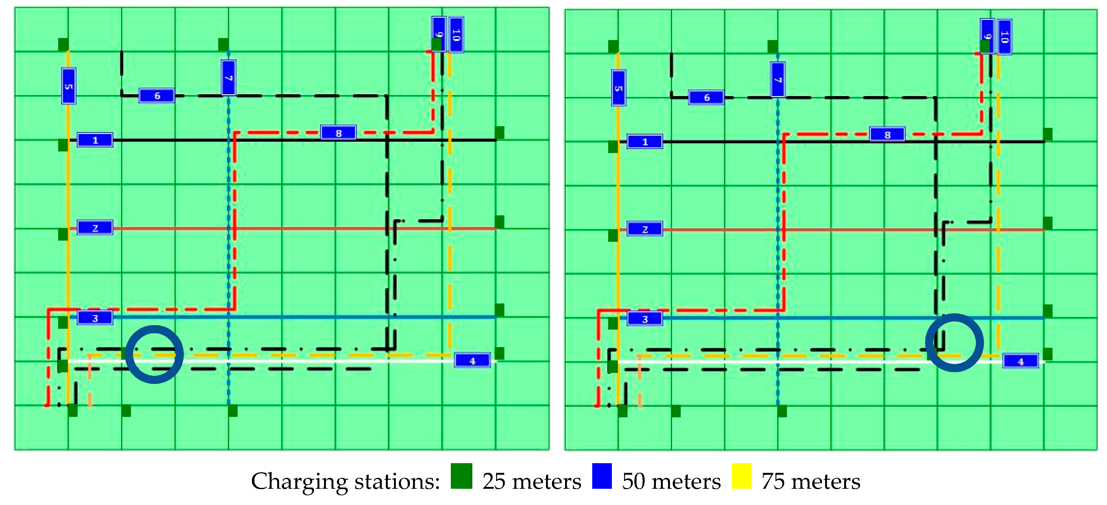
On the other hand, solutions 7 and 8 both used a 25 kWh battery, had the same cost (217,500$), and had the same total length of the electric bus route (93 km). The locations of the charging stations used in solutions 7 and 8 are presented in Figure 4 (solution 7—left, solution 8—right). As could be seen, in both solutions, there were 15 charging stations, with all charging stations being 25 m long. The difference between the two solutions lied in the location of one of the charging stations (marked with a circle in Figure 4). When choosing between these solutions, the decision-maker could further investigate the locations of the charging stations and could take into consideration other parameters that were difficult to integrate within the model (such as the likelihood of illegal parking at the bus stops).

6. Stochastic Variation of the Model

The term stochasticity refers to some source of randomness in a system. When considering a public transport system, there are several stochastic properties that should be considered. The two main stochastic properties that affect public-transport travel time are (1) traffic congestion and (2) dwell time.

Traffic congestion is a condition that is characterized by slower speeds, longer trip times, and increased vehicular queueing, and it occurs when the volume of traffic is greater than the available road capacity. For a given road, changes in traffic congestion are caused mainly by changes in the number of vehicles (due to weather conditions, car accidents, time of day, etc.). Dwell time refers to the length of time a public-transport bus spends at a scheduled stop without moving, usually for the boarding or alighting of passengers.

Since the calculations for the model presented above assumed average travel and dwell times, it is clear that due to the stochastic nature of traffic conditions and passenger behavior, in some cases, the discharge rate between two charging facilities will be higher than expected, while, in other cases, it will be lower. Consequently, the charging time at a specific charging facility may vary as well. That is, in the case where the power consumption is higher than expected, the bus driver may have to wait an additional length of time at some charging facilities. This, of course, may disrupt the bus schedule, increase the total travel time, and decrease reliability. In other cases, it is possible that the battery will be “overcharged”. This may happen when the power consumption is less than expected and/or the charging is higher than expected (e.g., due to a very long dwell time). This situation will lead to under-utilization of the charging facility. In such cases, the decision-maker may ask for solutions in which the additional dwell time and the total “overcharge” electric power are minimized. For that purpose, two additional objective functions were included in the model:

$$\begin{array}{ll}\min Z_4=& {\displaystyle \sum }_{i\in R}{\displaystyle \sum }_{j\in S}(\max \left(0,{\overline{w}}_{i,j}-w_{i,j}\right):F_{x_j}^{Charge}\left(\max \left(0,{\overline{w}}_{i,j}-w_{i,j}\right)\right)\\ & =\max (B_{i,j-1,j}^{Consumption}-{\overline{B}}_{i,j-1,j}^{Consumption},0)) \forall B_{i,j-1,j}^{Consumption}\\ & >{\overline{B}}_{i,j-1,j}^{Consumption}\end{array}$$

(10)

$$\min Z_5={\displaystyle \sum }_{i\in R}{\displaystyle \sum }_{j\in S}\max \left(E_{i,j}+F_{x_j}^{Charge}-B_b^{Size},0\right)$$

(11)

Suppose that $B_{i,j,k}^{Consumption}$ is the actual power consumed, and ${\overline{B}}_{i,j,k}^{Consumption}$ is the average power consumed for a bus on route $i$ traveling from bus stop $j$ to the next bus stop $k$. Using this notation, both $B_{i,j,0}$ and ${\overline{B}}_{i,j,0}$ are always equal to 0, where bus stop $0$ denotes the first bus stop on the route. Similarly, suppose that $w_{i,j}$ is the actual dwell time, and ${\overline{w}}_{i,j}$ is the average dwell time for a bus on route $i$ picking up passengers at bus stop $j$. To make sure that the energy level will be sufficient to arrive at the next charging facility, it is assumed that whenever $B_{i,j-1,j}^{Consumption}>{\overline{B}}_{i,j-1,j}^{Consumption}$ or $w_{i,j}<{\overline{w}}_{i,j}$, the driver, at bus stop $j$, waits an extra $t=\max \left(0,{\overline{w}}_{i,j}-w_{i,j}\right)$ seconds, such that $B_f^{Charge}\left(\max \left(0,w_{i,j}-{\overline{w}}_{i,j}\right)\right)=\max (B_{i,j-1,j}^{Consumption}-{\overline{B}}_{i,j-1,j}^{Consumption},0)$, where $f$ denotes the type of charging facility installed at bus station $j$. This notation is used by the first new objective, objective four, denoted by Equation (10), which minimizes the total added waiting time.

As mentioned above, $E_{ij}$ denotes the energy level of a bus on route $i$ arriving at bus stop $j$. Adding the amount of energy that is charged at bus stop $j$, $F_{x_j}^{Charge}\left(w_{i,j}\right)$, to $E_{i,j}$ yields the energy level of the battery of the bus on route $i$ when it leaves bus stop $j$. However, in the case where the battery cannot be overcharged, the term $E_{i,j}+F_{x_j}^{Charge}-B_b^{Size}$ has a positive value, compared to the regular negative or zero value. This notation is used by the second new objective, objective five, denoted by Equation (11), which minimizes the total “overcharging”.

It has been explained above that genetic algorithms are suitable for solving multi-objective optimization problems; however, they can be used for stochastic optimization problems as well.

Despite the ability of genetic algorithms to handle stochastic problems naturally, the approach used in this study was a little bit different. The first three objective functions were evaluated using the deterministic properties of the problem, while objective functions four and five were evaluated using the stochastic properties of the problem. To obtain realistic estimates of the values of objective functions four and five, these objectives were calculated a large number of times, using stochastic values of the travel time and the dwell time (which is different for every bus stop). The final values of the objectives were then taken to be the highest (i.e., worst case) values among those calculated.

The example problem described in Section 5 was solved twice: First, only with objectives one to four (without the consideration of the “overcharge” objective), and second, with all the objective functions. The result obtained using objective functions one to four was a Pareto set that included 456 non-dominated solutions.

Table 4. Sample of the non-dominated solutions for the test network.

Solution	Total Length (km) (Env. Impact)	Cost ($)	Number of Routes	Battery Size (kWh)	Total Waiting Time (s)	Number of Charging Facilities
						25 m	50 m	75 m
1	97	123,500	9	20	34,213	6	1	1
2	97	128,000	9	20	28,291	7	1	1
3	97	130,000	9	20	25,178	9	0	1
4	97	130,500	9	20	24,451	6	2	1
5	97	132,500	9	20	23,556	8	1	1
6	97	134,500	9	20	21,384	10	0	1
7	97	142,000	9	20	15,071	7	3	1
8	97	146,500	9	20	15,775	8	3	1
9	97	151,500	9	20	14,116	6	5	1
10	97	153,500	9	20	12,734	8	4	1
11	97	157,500	9	20	10,656	12	2	1
12	97	165,000	9	20	7180	9	5	1

provides a sub-set of the non-dominated solutions obtained for the test network. As could be seen, a sub-set had been chosen in which the total length of all solutions was 97 km, the number of routes that could be operated by electric buses was nine, and the battery size was 20 kWh. However, the total waiting time varied, and it was clear that it was negatively correlated with the cost of the solution; that is, the higher the cost of the solution, the lower the total waiting time (due to the additional charging capacity as a result of the additional costs).

7. Solution Set Ranking

Since the Pareto set of solutions is very large, multi-criteria decision-making techniques can be used to assist the decision-maker in ranking the solutions and selecting a preferred solution based on his/her preferences. Accordingly, the entire solution is comprised of the following steps, as described in Figure 5.

• Identify possible locations for charging facilities. This step also includes data collection about dwell time at each possible location and discharging rates between two consecutive locations.
• Apply the multi-objective genetic algorithm on previously collected data to determine the optimal locations of charging facilities.
• Apply MCDM on the result of the genetic algorithm to rank the solutions according to the DM preferences.
• Provide the results to the DM.

The TOPSIS (Technique for Order of Preference by Similarity to Ideal Solution) method [43] is a multi-criteria decision analysis method based on the assumption that the preferred solution should be closest to the ideal solution, $H^{*}$, and, at the same time, farthest from the negative ideal solution, $L_{*}$. For each alternative solution, the TOPSIS method calculates an index that is based on its position with respect to the ideal and negative ideal solutions. The alternative solution that maximizes this index value is the preferred alternative.

Given an evaluation matrix, $\theta$, consisting of n alternative solutions and m criteria, the first step of the TOPSIS method is the creation of a normalized matrix, R, from $\theta$, such that $r_{ij}={\theta }_{ij}/{\left(\sum _i{\theta }_{ij}^2\right)}^{0.5}$. Next, a weighted normalized decision matrix, $Q$, is computed such that $q_{ij}={\lambda }_j{r}_{ij}$, where ${\lambda }_j$ is the relative importance weight of the $j$^th criteria. The next step is to determine the ideal solution, $H^{*}$, and the negative ideal solution, $L_{*}$. The ideal solution is defined as $H^{*}=\left\{q_j^{*},j=1,2,\dots ,n\right\}=\left\{Max q_{ij},\forall i,j=1,2,\dots ,n\right\}$, while the negative ideal solution is defined as $L_{*}=\left\{q_j^{*},j=1,2,\dots ,n\right\}=\left\{Min q_{ij},\forall i,j=1,2,\dots ,n\right\}$. Based on the ideal and negative ideal solutions for each alternative solution, a separation measure, $P_i^{*}$, is calculated, such that $P_i^{*}={\left[\sum _i{\left(q_{ij}-q_j^{*}\right)}^2\right]}^{0.5}, i=1,2,\dots m$. Finally, based on the separation measure for each alternative solution, a similarity index, $D_i$, is calculated, such that $D_i=P_{*i}/\left(P_{*i}+P_i^{*}\right), i=1,2,\dots ,m$. A solution with a higher index value is preferred over one with a lower index value.

Assuming that all criteria are equally important (have the same weight), applying the TOPSIS method to the set of non-dominated solutions obtained for the test network ranks the solutions according to their relative importance.

Table 5. Best and worst solutions in the set of non-dominated solutions (objectives 1–4 only) for the test network based on TOPSIS (Technique for Order of Preference by Similarity to Ideal Solution).

Solution	Total Length (km) (Env. Impact)	Cost ($)	Number of Routes	Battery Size (kWh)	Total Waiting Time (s)
1	48	87,000	6	15	0
2	93	170,500	9	25	0
3	63	125,500	7	25	0
4	55	113,500	6	25	0
5	55	113,500	6	25	0
6	55	113,500	6	25	0
7	32	78,000	4	15	0
8	32	78,000	4	15	0
9	24	73,500	3	15	0
10	24	73,500	3	15	0
…
453	85	110,000	8	10	111,182
454	59	78,000	6	15	79,383
455	74	85,000	7	15	86,589

provides the top-ten best solutions (solutions 1 to 10) and the three worst solutions (solutions 453–455) according to the TOPSIS ranking, for the set of non-dominated solutions obtained for the test network in the case where objectives one to four were invoked. Similarly,

Table 6. Best and worst solutions in the set of non-dominated solutions (all five objectives) for the test network based on TOPSIS.

Solution	Total Length (km) (Env. Impact)	Cost ($)	Number of Routes	Battery Size (kWh)	Total Waiting Time (s)	Total Over-Charge (kWh)
1	24	104,500	3	25	0	0
2	24	104,500	3	25	0	0
3	24	104,500	3	25	0	0
4	32	109,000	4	25	0	0
5	32	109,000	4	25	0	0
6	32	109,000	4	25	0	0
7	32	109,000	4	25	0	0
8	32	109,000	4	25	0	0
9	40	116,000	5	25	0	0
10	40	116,000	5	25	0	0
…
4764	104	124,000	9	15	125,952	25,272
4765	39	67,500	4	10	67,309	13,984
4766	104	124,000	9	15	128,844	25,217

provides the top-ten best solutions (solutions 1 to 10) and the three worst solutions (solutions 4764–4766) according to the TOPSIS ranking for the case where all five objectives were invoked. As could be seen from Table 5 and Table 6, the TOPSIS method ranked solutions for which the total waiting time and total over-charge were equal to zero as the best solutions.

8. Conclusions

A multi-objective model for the allocation of wireless bus charging stations was proposed. The model development was motivated by the increasing popularity of wireless charging in transportation. For example, the Israeli start-up company Electreon developed a dynamic wireless electrification system for electric transportation. Their initial focus was on public transport and heavy trucks, as these vehicles usually operate on fixed, known routes. The company manages projects both in Israel and Sweden.

Unlike previous models that deal with a single objective and consider either a single route or the whole network, the current model introduced several objective functions that provided the decision-maker with the flexibility to decide which routes to electrify. Moreover, with such a tool, it is possible to prioritize the electrification phases of the whole network, which is beneficial, given that such a project can take considerable time. Finally, the model took into consideration the environmental contribution of the electrification based on pollution and noise reduction; hence, the prioritization is not based solely on costs, but also on sustainability.

Further research could consider a more detailed analysis of the charging characteristics of online and offline bus stops, as well as priority lanes. Furthermore, actual data related to energy consumption, speed, and costs could be used by collecting data from the operation of electric shuttles at the Bar-Ilan University campus and electric buses operating in Israel.

References

- Lebeau, K.; Van Mierlo, J.; Lebeau, P.; Mairesse, O.; Macharis, C. Consumer attitudes towards battery electric vehicles: A large-scale survey. Int. J. Electr. Hybrid Veh. 2013, 5, 28–41. [Google Scholar] [CrossRef]
- Hui, S.Y.; Lee, C.K.; Wu, F.F. Electric springs—A new smart grid technology. IEEE Trans. Smart Grid 2012, 3, 1552–1561. [Google Scholar] [CrossRef] [Green Version]
- Dyke, K.J.; Schofield, N.; Barnes, M. The impact of transport electrification on electrical networks. IEEE Trans. Ind. Electron. 2010, 57, 3917–3926. [Google Scholar] [CrossRef]
- Wu, G.; Boriboonsomsin, K.; Barth, M.J. Development and evaluation of an intelligent energy-management strategy for plug-in hybrid electric vehicles. IEEE Trans. Intell. Transp. Syst. 2014, 15, 1091–1100. [Google Scholar] [CrossRef]
- Rigas, E.S.; Ramchurn, S.D.; Bassiliades, N. Managing electric vehicles in the smart grid using artificial intelligence: A survey. IEEE Trans. Intell. Transp. Syst. 2014, 16, 1619–1635. [Google Scholar] [CrossRef]
- Sinhuber, P.; Rohlfs, W.; Sauer, D.U. Study on power and energy demand for sizing the energy storage systems for electrified local public transport buses. In Proceedings of the 2012 IEEE Vehicle Power and Propulsion Conference, Seoul, South Korea, 9–12 October 2012; pp. 315–320. [Google Scholar]
- Kowalenko, K. Going Electric: Things to Consider; IEEE-The Institute: Piscataway, NJ, USA, 2011. [Google Scholar]
- Ulrich, L. State of charge. IEEE Spectr. 2012, 49, 56–59. [Google Scholar] [CrossRef]
- Wikipedia Contributors. BYD K9 Official Specifications. Available online: https://en.wikipedia.org/wiki/BYD_K9#Official_specifications (accessed on 31 July 2019).
- Xylia, M.; Leduc, S.; Patrizio, P.; Silveira, S.; Kraxner, F. Developing a dynamic optimization model for electric bus charging infrastructure. Transp. Res. Procedia 2017, 27, 776–783. [Google Scholar] [CrossRef] [Green Version]
- Xylia, M.; Leduc, S.; Patrizio, P.; Kraxner, F.; Silveira, S. Locating charging infrastructure for electric buses in Stockholm. Transp. Res. Part C Emerg. Technol. 2017, 78, 183–200. [Google Scholar] [CrossRef]
- Jang, Y.J.; Jeong, S.; Ko, Y.D. System optimization of the on-line electric vehicle operating in a closed environment. Comput. Ind. Eng. 2015, 80, 222–235. [Google Scholar] [CrossRef]
- Jang, Y.J.; Suh, E.S.; Kim, J.W. System architecture and mathematical models of electric transit bus system utilizing wireless power transfer technology. IEEE Syst. J. 2015, 10, 495–506. [Google Scholar] [CrossRef]
- Liu, Z.; Song, Z. Robust planning of dynamic wireless charging infrastructure for battery electric buses. Transp. Res. Part C Emerg. Technol. 2017, 83, 77–103. [Google Scholar] [CrossRef]
- Song, Z. Transition to a transit city: Case of Beijing. Transp. Res. Rec. 2013, 2394, 38–44. [Google Scholar] [CrossRef]
- Bolger, J.; Kirsten, F.; Ng, L. Inductive power coupling for an electric highway system. In Proceedings of the 28th IEEE Vehicular Technology Conference, Denver, CO, USA, 22–24 March 1978; pp. 137–144. [Google Scholar]
- Esser, A. Contactless charging and communication for electric vehicles. IEEE Ind. Appl. Mag. 1995, 1, 4–11. [Google Scholar] [CrossRef]
- Ayano, H.; Yamamoto, K.; Hino, N.; Yamato, I. Highly efficient contactless electrical energy transmission system. In Proceedings of the IEEE 2002 28th Annual Conference of the Industrial Electronics Society. IECON 02, Sevilla, Spain, 5–8 November 2002; pp. 1364–1369. [Google Scholar]
- Wu, H.H.; Boys, J.T.; Covic, G.A. An AC processing pickup for IPT systems. IEEE Trans. Power Electron. 2009, 25, 1275–1284. [Google Scholar] [CrossRef]
- Budhia, M.; Covic, G.A.; Boys, J.T. Design and optimization of circular magnetic structures for lumped inductive power transfer systems. IEEE Trans. Power Electron. 2011, 26, 3096–3108. [Google Scholar] [CrossRef]
- Huang, C.-Y.; Boys, J.T.; Covic, G.A.; Budhia, M. Practical considerations for designing IPT system for EV battery charging. In Proceedings of the 2009 IEEE Vehicle Power and Propulsion Conference, Dearborn, MI, USA, 7–10 September 2009; pp. 402–407. [Google Scholar]
- Lee, S.; Huh, J.; Park, C.; Choi, N.-S.; Cho, G.-H.; Rim, C.-T. On-line electric vehicle using inductive power transfer system. In Proceedings of the 2010 IEEE Energy Conversion Congress and Exposition, Atlanta, GA, USA, 12–16 September 2010; pp. 1598–1601. [Google Scholar]
- Shin, J.; Shin, S.; Kim, Y.; Ahn, S.; Lee, S.; Jung, G.; Jeon, S.-J.; Cho, D.-H. Design and implementation of shaped magnetic-resonance-based wireless power transfer system for roadway-powered moving electric vehicles. IEEE Trans. Ind. Electron. 2013, 61, 1179–1192. [Google Scholar] [CrossRef]
- Ip, A.; Fong, S.; Liu, E. Optimization for allocating BEV recharging stations in urban areas by using hierarchical clustering. In Proceedings of the 2010 6th International Conference on Advanced Information Management and Service (IMS), Seoul, South Korea, 30 November–2 December 2010; pp. 460–465. [Google Scholar]
- Ge, S.; Feng, L.; Liu, H. The planning of electric vehicle charging station based on grid partition method. In Proceedings of the 2011 International Conference on Electrical and Control Engineering, Yichang, China, 16–18 September 2011; pp. 2726–2730. [Google Scholar]
- Kristoffersen, T.K.; Capion, K.; Meibom, P. Optimal charging of electric drive vehicles in a market environment. Appl. Energy 2011, 88, 1940–1948. [Google Scholar] [CrossRef]
- Steinmauer, G.; Del Re, L. Optimal control of dual power sources. In Proceedings of the 2001 IEEE International Conference on Control Applications (CCA’01)(Cat. No. 01CH37204), Mexico City, Mexico, 7 September 2001; pp. 422–427. [Google Scholar]
- Tate, E.D.; Boyd, S.P. Finding ultimate limits of performance for hybrid electric vehicles. SAE Trans. 2000, 2437–2448. [Google Scholar]
- Riemann, R.; Wang, D.Z.; Busch, F. Optimal location of wireless charging facilities for electric vehicles: Flow-capturing location model with stochastic user equilibrium. Transp. Res. Part C Emerg. Technol. 2015, 58, 1–12. [Google Scholar] [CrossRef]
- Liu, H.; Wang, D.Z. Locating multiple types of charging facilities for battery electric vehicles. Transp. Res. Part B Methodol. 2017, 103, 30–55. [Google Scholar] [CrossRef]
- Marler, R.T.; Arora, J.S. Survey of multi-objective optimization methods for engineering. Struct. Multidiscip. Optim. 2004, 26, 369–395. [Google Scholar] [CrossRef]
- Zadeh, L. Optimality and non-scalar-valued performance criteria. Autom. Control IEEE Trans. 1963, 8, 59–60. [Google Scholar] [CrossRef]
- Stadler, W. Fundamentals of multicriteria optimization. In Multicriteria Optimization in Engineering and in the Sciences; Springer: Berlin/Heidelberg, Germany, 1988; pp. 1–25. [Google Scholar]
- Das, I.; Dennis, J. An improved technique for choosing parameters for Pareto surface generation using normal-boundary intersection. In Proceedings of the Short Paper Proceedings of the Third World Congress of Structural and Multidisciplinary Optimization, Buffalo, NY, USA, 17–21 May 1999; pp. 411–413. [Google Scholar]
- Das, I.; Dennis, J.E. Normal-boundary intersection: A new method for generating the Pareto surface in nonlinear multicriteria optimization problems. SIAM J. Optim. 1998, 8, 631–657. [Google Scholar] [CrossRef] [Green Version]
- Messac, A.; Ismail-Yahaya, A.; Mattson, C.A. The normalized normal constraint method for generating the Pareto frontier. Struct. Multidiscip. Optim. 2003, 25, 86–98. [Google Scholar] [CrossRef]
- Yu, P.-L. A class of solutions for group decision problems. Manag. Sci. 1973, 19, 936–946. [Google Scholar] [CrossRef]
- Coello, C.A.C.; Lamont, G.B.; Van Veldhuizen, D.A. Evolutionary Algorithms for Solving Multi-Objective Problems; Springer-Verlag New-York Inc.: New York, NY, USA, 2007. [Google Scholar]
- Yoshitomi, Y.; Ikenoue, H.; Takeba, T.; Tomita, S. Genetic algorithm in uncertain environments for solving stochastic programming problem. J. Oper. Res. Soc. Jpn. 2000, 43, 266–290. [Google Scholar] [CrossRef] [Green Version]
- Żak, J.; Kruszyński, M. Application of AHP and ELECTRE III/IV methods to multiple level, multiple criteria evaluation of urban transportation projects. Transp. Res. Procedia 2015, 10, 820–830. [Google Scholar] [CrossRef] [Green Version]
- Ehrgott, M. Multicriteria Optimization; Springer: Berlin/Heidelberg, Germany, 2005. [Google Scholar]
- Roy, B. Decision-aid and decision-making. Eur. J. Oper. Res. 1990, 45, 324–331. [Google Scholar] [CrossRef]
- Hwang, C.L.; Yoon, K. Multiple Attribute Decision Making: Methods and Applications A State-of-the-Art Survey; Springer: New York, NY, USA, 1981; Volume 13. [Google Scholar]
- Roy, B. The outranking approach and the foundations of ELECTRE methods. Theory Decis. 1991, 31, 49–73. [Google Scholar] [CrossRef]
- Keeney, R.L.; Raiffa, H.; Rajala, D.W. Decisions with multiple objectives: Preferences and value trade-offs. IEEE Trans. Syst. Man Cybern. 1979, 9, 403. [Google Scholar] [CrossRef]
- Masud, A.S.M.; Ravindran, A.R. Multiple Criteria Decision Making. In Operations Research and Management Science Handbook; Ravindran, A.R., Ed.; Taylor & Francis Group, LLC: Abingdon, UK, 2008. [Google Scholar]
- Saaty, T.L. A scaling method for priorities in hierarchical structures. J. Math. Psychol. 1977, 15, 234–281. [Google Scholar] [CrossRef]
- Saaty, T.L. Decision making with the analytic hierarchy process. Int. J. Serv. Sci. 2008, 1, 83–98. [Google Scholar] [CrossRef] [Green Version]
- Saaty, T.L. Analytic network process. In Encyclopedia of Operations Research and Management Science; Springer: Berlin/Heidelberg, Germany, 2001; pp. 28–35. [Google Scholar]
- Schaffer, J.D. Multiple objective optimization with vector evaluated genetic algorithms. In Proceedings of the 1st international Conference on Genetic Algorithms, Pittsburgh, PA, USA, 24–26 July 1985; pp. 93–100. [Google Scholar]
- Schaffer, J.D.; Grefenstette, J.J. Multi-objective learning via genetic algorithms. In Proceedings of the Ninth International Joint Conference on Artificial Intelligence, Los Angeles, CA, USA, 19–23 August 1985; pp. 593–595. [Google Scholar]
Figure 1.
Separate (left) versus joint (right) allocation of charging stations.
Figure 2.
The public transport (PT) network.
Figure 3.
Locations of the charging stations for solutions 6 (left) and 9 (right).
Figure 4.
Location of the charging stations for solutions 7 (left) and 8 (right).
Figure 5.
Flowchart describing the process of finding optimal locations of charging facilities.