Analysis of the Habitat Fragmentation of Ecosystems in Belize Using Landscape Metrics


1
Department of Bioenvironmental Systems Engineering, National Taiwan University, Taipei 10617, Taiwan
2
School of Natural and Environmental Sciences, Newcastle University, Newcastle upon Tyne NE17RU, UK
*
Author to whom correspondence should be addressed.
Sustainability 2020, 12(7), 3024; https://0-doi-org.brum.beds.ac.uk/10.3390/su12073024
Submission received: 9 March 2020
/
Revised: 5 April 2020
/
Accepted: 8 April 2020
/
Published: 9 April 2020
(This article belongs to the Special Issue Landscape Fragmentation and Sustainable Environmental Assessment)
Abstract
:Landscape metrics have been of game changing importance in the analysis of ecosystems’ composition and landscape cohesion. With the increasing urban and agricultural expansion, the natural flora and fauna of many highly diverse areas have been degraded. Fragmentation of ecosystems and habitats have stressed the biodiversity of Belize. To understand the dynamics of this change, a study was conducted using three moderately separate years of ecosystem landscape data. The metrics used for the analysis were area-weighted mean shape index (AWMSI), mean shape index (MSI), edge density (ED), mean patch size (MPS), number of patches (NUMP), and class area (CA). These metrics were produced for the years 2001, 2011, and 2017. The classes of agricultural use, lowland savannas, mangroves and littoral forests, urban, and wetlands were the subjects for analysis. Using the GIS extension Patch Analyst, parametric runs were performed. From these results, a one-way ANOVA test of the NUMP, Tukey HSD test, and Scheffé Multiple Comparison test were performed. The results indicate that there has been significant habitat fragmentation, especially from the years 2001 to 2011. Agricultural areas increased by 19.37% in just 10 years, with the NUMP of some habitats increasing by 284%. The results also show fluctuation in ED and a decrease in overall MPS, all indicating high fragmentation. These changes have been mostly induced due to the expansion of agricultural activities and urbanization, especially in the northern parts of Belize. It is imperative that additional policies be implemented to deter the effects of habitat fragmentation upon the existing ecosystems of Belize and elsewhere.
1. Introduction
1.1. Habitat Fragmentation
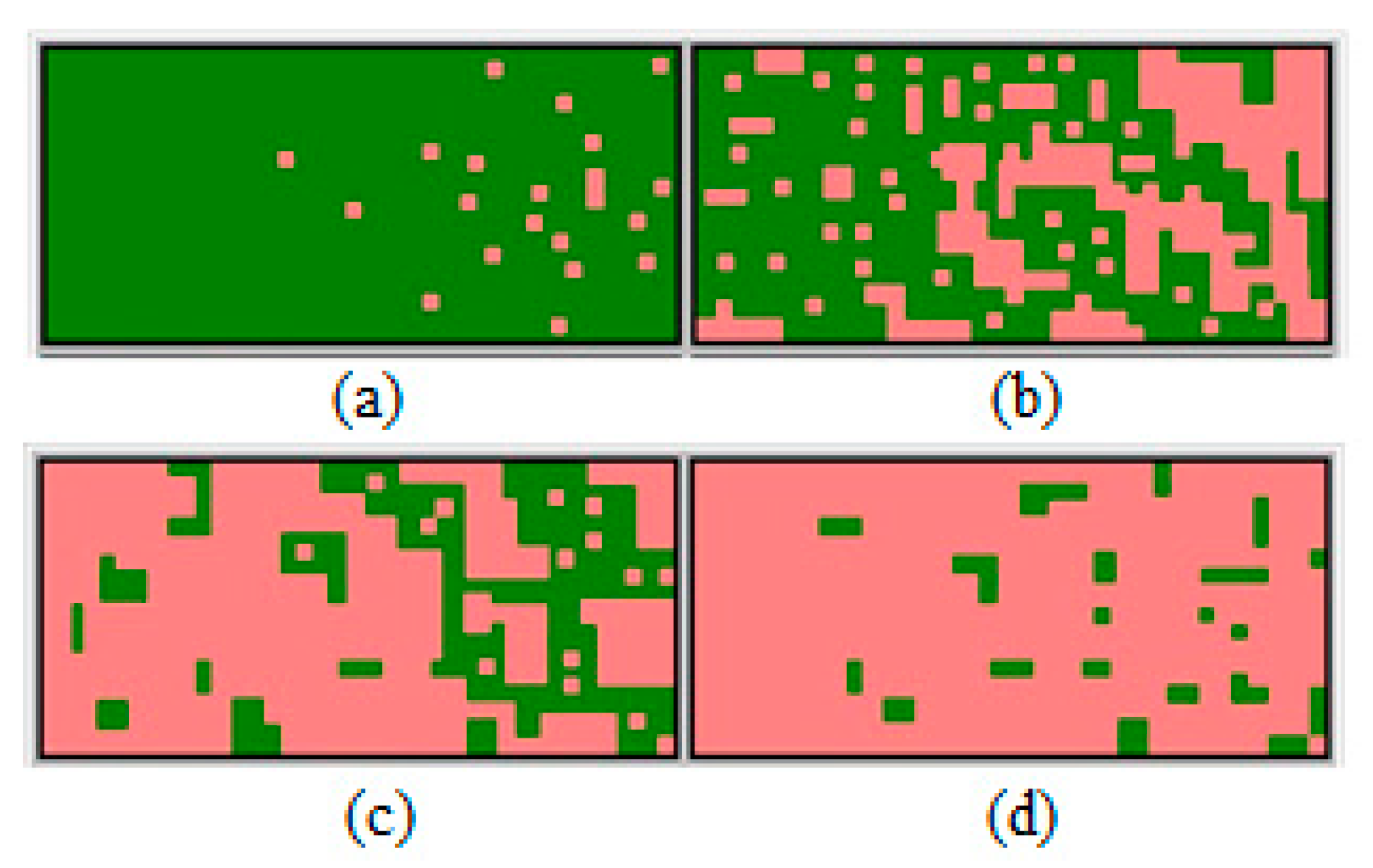
When natural habitat is altered, both its composition and configuration change. This change is called fragmentation [1]. Habitat breakages or the degree of patchiness of a habitat is a result of anthropogenic activities [2]. These activities can result in higher probabilities of local extinction with lower probabilities of recolonization [3]. As anthropogenic pressures continuously contract habitual areas, the ecosystems within these areas become drastically disrupted and degraded. The process of this degradation can be summarized in four stages: perforation, dissection, dissipation, and shrinkage (Figure 1). These impacts are mainly influenced by the increment of land use [4]. This use refers to all components of change in the quantity and quality of land cover types as habitats for organisms and productive land for humans [5]. Several models developed have indicated that there exists a negative effect on species population growth rate, which dictates that decreasing trends in abundance are more likely to occur in areas with high habitat loss [6,7]. Although there has been considerable focus on the global status of these species, true importance lies in the longevity and security of these ecosystems in the changing environments, which depend on local biodiversity [8]. This local diversity can be assessed and studied with landscape pattern analysis, which measures the arrangement and composition of habitats and ecosystems [9]. Some studies (such as [10,11,12,13]) have conducted studies about deforestation and diversity in Belize. However, these studies did not employ the use of landscape metrics to assess habitat fragmentation. This research employed landscape metrics in studying the habitat fragmentation variations to provide a different perspective on the status of Belize ecosystems.
1.2. Landscape Metrics
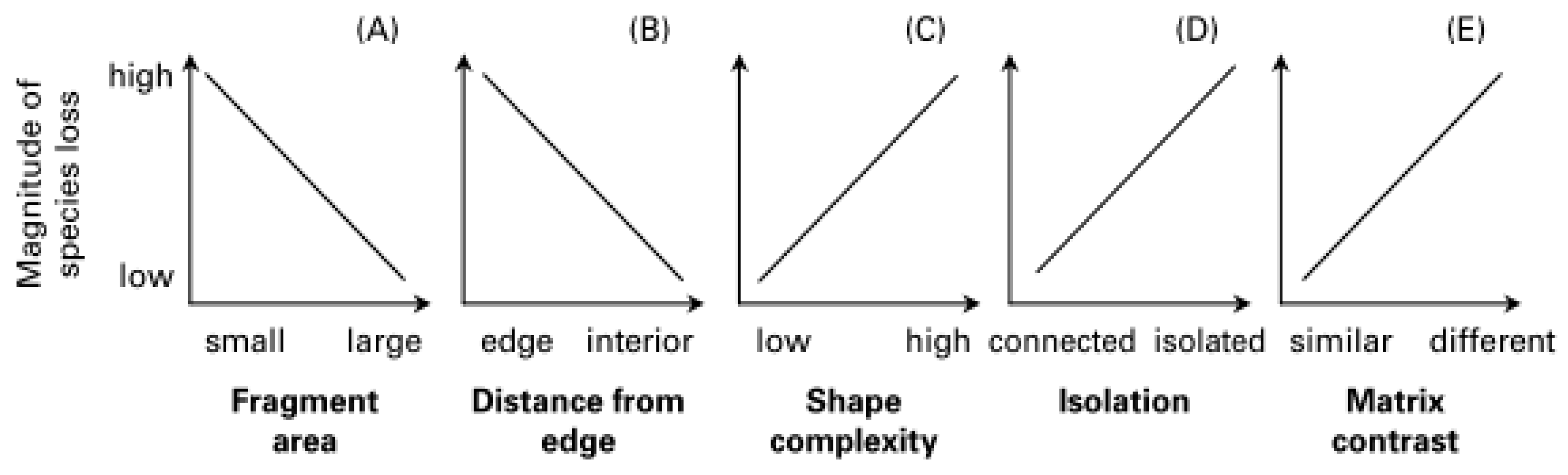
Spatial pattern metrics are used to measure the organization of habitats within a landscape. Such studies as [10] have allowed ecologists to establish tangible relationships between very important landscape indices, and thus, have become important tools in ecological research [11]. Landscape metrics are also important in understanding the dynamics of anthropogenic interaction with natural habitats and urban expansion [12,13]. Their speed of calculation and their simplicity have been some of the main advantages of landscape metrics [14]. In the process of understanding the dynamics of landscapes, there have been developments and well-established generalizations concerning the response of ecosystems to habit fragmentation [15,16]. These responses, as observed in Figure 2, either represent an increase or a decrease in the magnitude of species loss. Metrics such as class area (CA) and mean patch size (MPS) describe the area of a patch or fragment within a landscape. Decreases in the area of patches are synonymous with increases in habitat fragmentation. To describe shape complexity of patches, there are several indices. Some of these include shape index (SHAPE), mean shape index (MSI), area-weighted mean shape index (AWMSI), landscape shape index (LSI), just to name a few. These metrics describe how complex patches are, where an increase in complexity leads to an increase in fragmentation. Like shape complexity, high numbers in distance from the edge of a habitat indicate a fragmented ecosystem. Metrics such as edge density (ED) describe the distance of an ecosystem from its centroid, meaning the center of the patch.
1.3. Study Area and Aim
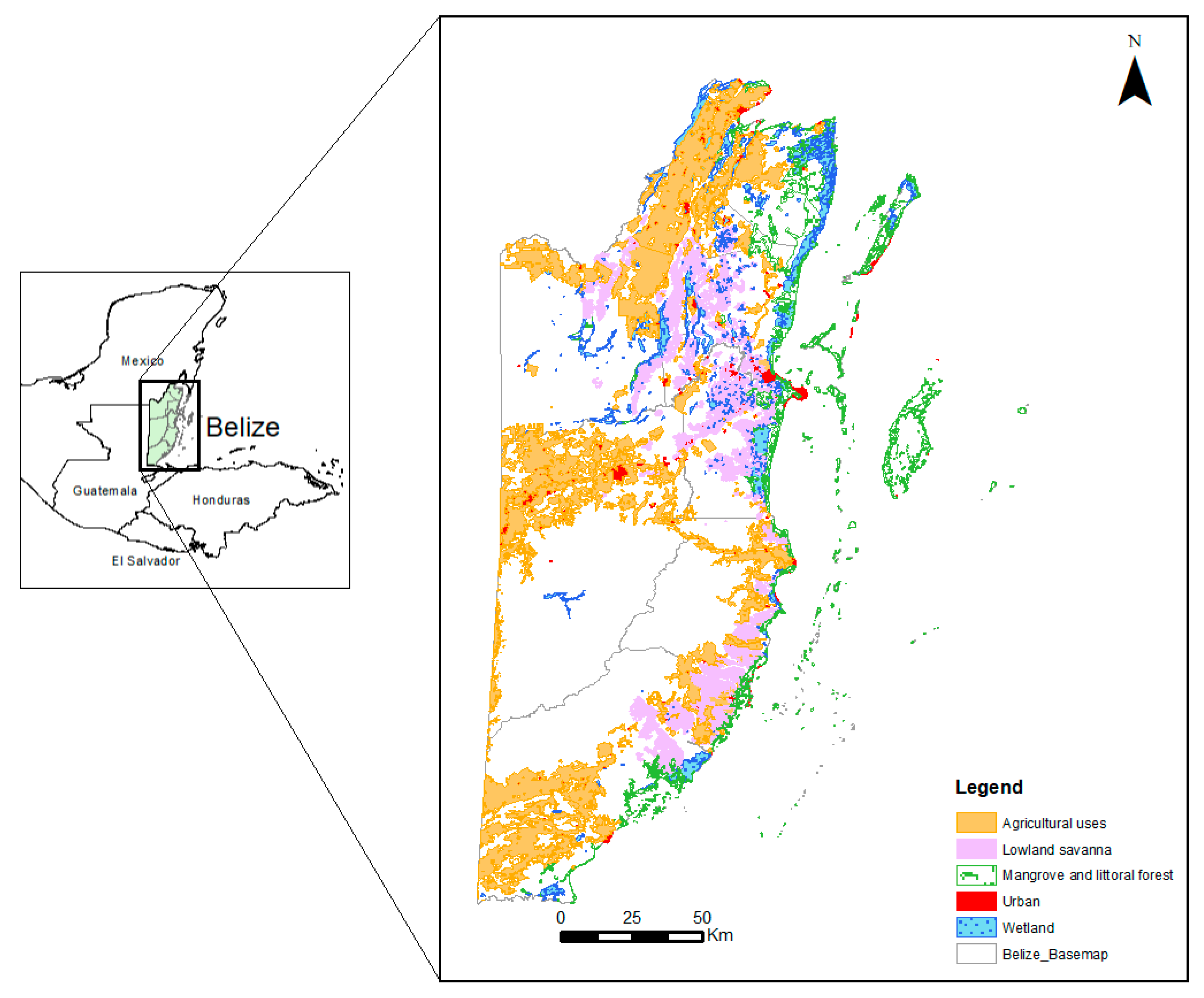
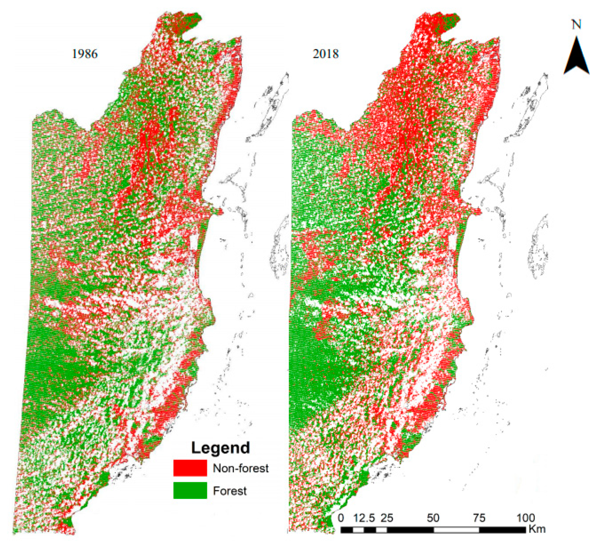
Anthropogenic activities have plagued most existing ecosystems, and such has been the case in Central America, particularly Belize. Over 60% of Belize’s land surface is covered by forest [18]. Around 20% of the country’s land is covered by cultivated land (agriculture) and human settlements, while the savannas, scrublands, and wetlands constitute the remainder of Belize’s land cover [19]. This can be observed in Figure 3. Settlement and agricultural land expansion have caused heavy pressure to be put upon the ecosystems of Belize [20,21]. A notable change in the forest area can be seen in Figure 4 which shows the forest cover in Belize in 1986 and in 2018. The images were created by the authors in [22] and were derived from Landsat data. The figure shows forest cover over the entire country. The 1984 images were collected by the Thematic Maper (TM) aboard Landsat 5, the 2018 images were by the Enhanced Thematic Mapper (ETM+) Plus aboard Landsat 7. Both images are at a resolution of 30 m. The figure on the right (Figure 4b) resembles the first and second phases of fragmentation, perforation, and dissection, respectively. The total protected areas in Belize, both terrestrial and aquatic, amount to some 47%, including the Belize Barrier Reef [23]. As Belize consists of habitats that host endangered and threatened species, habitat fragmentation has been especially challenging to conservation efforts [24]. A few studies have been done that focus on the fragmentation of ecosystems in Belize, such as [25], but these studies did not employ the use of landscape metrics. Therefore, the aim of this study is to analyze habitat fragmentation in Belize using different landscape indices from the years 2001, 2011, and 2017. The results will aid in understanding the transformation of the Belize landscape throughout the stated years, in addition to exploring what type of transformations have taken place throughout that time. It is also our aim to determine which factors have led to the change in the landscapes, and if there has been fragmentation, by how much has it increased or decreased through the years. It is essential to this study to determine the aforementioned in hope that it represents a practical assessment of the conditions of the Belize landscape and of the efficacy of the protection policies previously implemented to stop habitat fragmentation.
2. Materials and Methods
2.1. Spatial Data
The shapefiles that represented the ecosystems of Belize for the years of 2001, 2011, and 2017 were produced at different times and with different accuracies and resolutions. The map which represented the ecosystems for the year 2001 was produced by Meerman and Sabido in 2001. The map was essentially an update of a vegetation map produced in 1995. The map for 2011 was an update of the map produced in 2001. Some changes made to update the map included using fieldwork data gathered by the authors from 2001 to 2004, updated Landsat TM images, revised vegetation classification, climatological data attained from the MET department and a geology map of Belize produced by Cornec in 2003 [19]. The map that represents ecosystems in Belize for 2017 was basically an improvement of the maps produced the previous years. This version, however, was based on February 2017 Landsat 8 imagery augmented with numerous online high-resolution imageries. The trend has been as previous iterations, to improve the resolution and accuracy [26].
The shapefiles are in reference to the Universal Transverse Mercator (UTM) with the geodetic datum being the North American Datum of 1927 (NAD27) Zone 16 North [26]. The Digital Elevation Model (DEM) data for Belize was attained from the Caribbean Handbook on Risk Information Management (CHARIM) GeoNode [27]. The spatial resolution of the DEM was 90 m. To determine the extent of breakage in the biological corridor, the Patch Analyst 5.2 was used. The Patch Analyst is a program extension in the ArcGIS® software system that is a part of the Spatial Ecology section developed by the Centre for Northern Forest Ecosystem Research (CNRER) in Canada. It facilitates the spatial analysis of landscape patches and the modeling of attributes associated with patches [28]. To initiate the process, the BERDS shapefiles were loaded into ArcGIS 10.1 [29] and prepared for patch analysis. After the analysis type was defined, the program was executed. Individual fragmentation analysis were done for the years 2001, 2011 and 2017 in the Patch Analyst 5.2 [28]. All runs were done at the ‘class level’, which serves to quantify the landscape composition and configuration of landscapes [30]. The fragmentation metrics that were of particular interest were chosen based upon their correspondence to the evaluation of ecosystem fragmentation and their use by authors in studies briefly mentioned in Section 1.2. These metrics are further explained in Section 2.2.
2.2. Fragmentation Metrics and Landscape Classes Used in the Study
The classes or patch types that were selected from the shapefiles with the ecosystem polygons were agricultural uses (AU), lowland savanna (LS), mangrove and littoral forests (MLF), urban (URB), and wetlands (WL). Although the BERDS data bank contains several shapefiles with extensive spatial data, there was a slight hiccup with the representation of the classes across the years. Some classes were present in some years which were not present in the other years. LS, MLF, and WL were chosen as the biotic landscape classes because they were present in all 3 shapefiles for the respective years. The remaining 2 classes, AU and URB, were selected specifically for their independence. Since these 2 classes expanded and were expected to do so dramatically with time, it is possible that they marginalized and edged the surrounding ecosystems. This can be particularly so for LS since its terrain and fertility facilitate good farming.
As previously stated, the most important categorical landscape metrics for determining habitat fragmentation are habitat area, edge effects, and shape complexity [31]. It was imperative to select metrics that fit these categories. For habitat or fragment area, the CA and the MPS were selected. The CA and MPS are measured in hectares. For shape complexity, the AWMSI and MSI were used. Both metrics are similar in that they are equal to 1 when the patches of corresponding patch type are circular or square, but the AWMSI is weighted by patch area so the larger patches will weigh more than smaller ones [32]. To determine the edge effects, the ED metric was used. The ED indicates the amount of edge relative to the landscape area. The final metric selected was number of patches (NUMP). This was perhaps one of the most important metrics since its determination is clear and straightforward. An increase or decrease in the NUMP would indicate an increase or decrease in habitat fragmentation, respectfully.
The following subsection discusses each metric, presents its formula and provides a brief description as to their relation to landscape metric analysis. The metrics are presented here as they were originally presented by McGarigal et al. in 1995 for the development of FRAGSTATS (Spatial Pattern Analysis for Program for Quantifying Landscape Structure) [32].
2.2.1. ED (Edge Density)
The formula for ED is shown below as Equation (1). The ED equals the sum of the lengths (m) of all edge segments that correspond the particular patch type, divided by the total landscape area (m2), and by 10,000 (to convert to hectares).
where is the total length (m) of the edge in the landscape involving patch type (class) which includes landscape boundary and background segments involving patch type , and is the total landscape area (m2). The value of ED can be 0, which signifies that there is no edge in the landscape class. The value is non-zero when there is change in class edge. ED is measured in meters/hectare (m/ha).
2.2.2. MPS (Mean Patch Size)
The mean patch size is equal to the sum of all patches of the corresponding patch type, of the particular patch metric values, divided by the number of patches of the same type, divided by 10,000 (to convert to hectares),
where is the number of patches in the landscape of patch type (class) , and is the area of patch . The mean patch size has a unit of hectares and is a non-zero value with no limit.
2.2.3. NUMP (Number of Patches)
The NUMP simply equals the number of patches of the corresponding patch type (class) and is represented as Equation (3). The number of patches of a particular patch type is a simple measure of the extent of subdivision or fragmentation of the patch type. The NUMP = 1 when the landscape contains only 1 patch. This number has no units and no limits.
2.2.4. AWMSI (Area-Weighted Mean Shape Index)
The AWMSI is equivalent to the sum, across all patches of the corresponding patch type, of each patch perimeter (m) divided by the square root of patch area (m2), adjusted by a constant to adjust for a circular standard (vector) multiplied by the patch area (m2) divided by total class area (sum of patch area for each patch of the corresponding patch type). The AWMSI, in other words, is the average shape index of the corresponding patch type, weighted by size so that larger patches weigh more than smaller ones. This is represented as Equation (4).
where is the perimeter (m) of patch . The AWMSI is 1 when all the patches of the corresponding patch type are circular (when vector, as in our study) or square (when raster). The AWMSI has no unit and no limit. Equation (4) differs slightly if the spatial data are represented as raster.
2.2.5. MSI (Mean Shape Index)
The MSI is equal to the sum of the patch perimeter (m) divided by the square root of patch area (m2) for each patch of the corresponding patch type, adjusted the same way as the AWMSI described in Section 2.2.4. The MSI is represented as:
where known variables are the same as those stated in Section 2.2.4. The MSI is equal to 1 when all of the patches of the corresponding patch are circular (when vector, as in our study) or square (when raster). The same applies as in Section 2.2.4, where Equation (5) would differ slightly were the data are represented as raster. The MSI = 1 when all patches of the corresponding patch type are circular (vector, in our study), and has no limit or unit.
2.2.6. CA (Class Area)
The class area equals the sum of the areas (m2) of all patches of the corresponding patch type, divided by 10,000; that is, the total class area. The formula of the CA is represented as Equation (6),
where is the area (m2) of patch . The CA approaches zero as the patch type becomes increasingly rare in the landscape. The larger the CA, the more unified the patch type. The CA has the unit of hectares (ha) and no limit.
2.3. Data Analysis
A one-way analysis of variance (ANOVA) test was done with the NUMP [33]. This method of analysis was chosen following a study of similar direction [33]. The NUMP was chosen as the primary source of data for the ANOVA since it is the most indicative metric relative to fragmentation. The NUMP also has the quality of simplicity. Either it increases or decreases as the other metrics do, but its direction provides a prelude to the condition of the habitat. The ANOVA was ‘between groups’ across the 3 years of metrics data gathered from the Patch Analyst evaluation. The analysis of the NUMP ‘between groups’ indicates that the source of the variation in the ANOVA was obtained from the comparison of the values by years, not individual landscape type or class. Therefore, values from 2001, 2004, and 2017 were compared as groups. Although change is visible (as previously observed in Figure 4) and there was a high expectation that there was change, a comparison of the variance of these groups was necessary to consolidate this expectation. It was necessary to determine which pairing expressed the most significant difference.
A post-hoc test is usually used to uncover specific differences between three or more group means when the ANOVA test proves to be significant. There are several types of post-hoc tests. A few are used with more regularity than others. Some post-hoc tests are Tukey’s honest significance test (Tukey HSD), Duncan, Student-Newman-Keuls (SNK), least significant difference (LSD), and Scheffé Multiple Comparison. The Scheffé Multiple Comparison test is the most protective against Type 1 error [34]. For this, this test was deemed appropriated. A Tukey HSD test was also done to have high confidence in the results.
3. Results
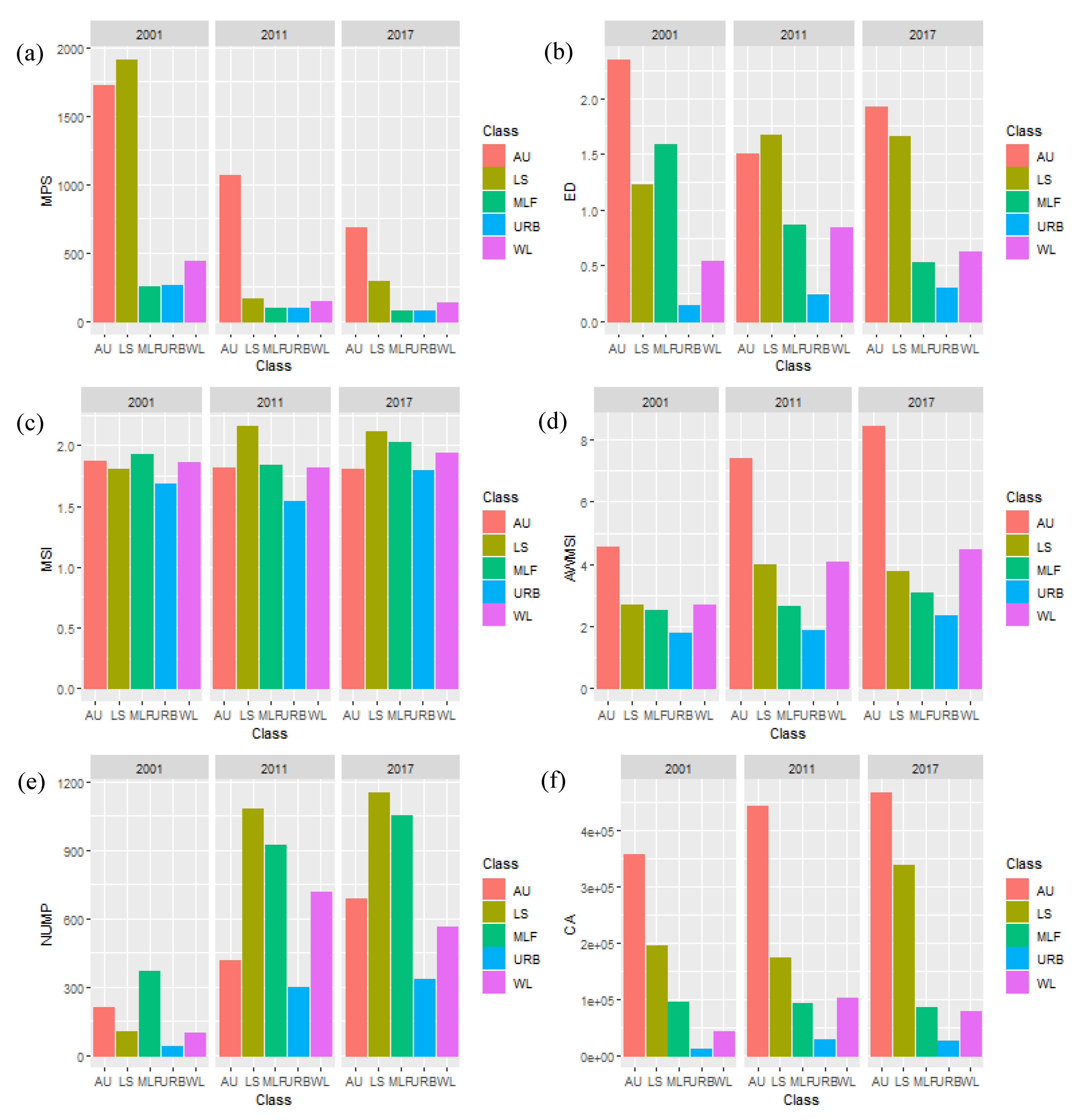
All results were from the Patch Analyst runs for the years 2001, 2011, and 2017. The results can be seen in Figure 5. Since the runs were done year by year, the results were grouped as such. A value was generated for each metric under every class for each year. Were the landscape static, these numbers would remain roughly the same throughout the years. The hyper-change of the values of almost all metrics indicate that there has been habitat modification. Although some of the metric values that are indicative of habitat cohesion are close to 1, any slight variation in their numbers indicates a large difference. The most numerically significant is the CA, as expected, since it represents area. A change in CA, as can has been explained in Section 2.2, is synonymous with changes in landscape composure. To have a more visual understanding of this, the results from the runs in the Patch Analyst were summarized graphically in Figure 5. The exact values of the key metrics can be seen in Table A1 in the Appendix A. The results are shown as such that for every metric, the results are for every year of every class. This was done so that the increase or decrease in each metric is easily decipherable.
The results of the ANOVA are presented in Table 1. For a p-value of 0.0120, the results indicate that there is a significant difference between the number of patches of the classes through the years between 2001, 2011, and 2017. To determine where the difference was most drastic or statistically significant, it is necessary to look at the post-how results summarized in Table 2. Both the Tukey HSD test and Scheffé multiple comparison generated the same results, which indicate that the most drastic change was between the years 2001 and 2011. The year-pairs 2011 vs. 2017, however, showed that the change was insignificant. This was also the result for both post-hoc tests, as is observed in Table 2.
4. Discussion and Conclusions
The results show that there was a significant change for all the biotic classes from the years 2001 to 2017. They indicate overall fragmentation in all classes. The ANOVA results attained from the test between groups of years showed that the populations from datasets of years 2001 and 2011 were significantly uneven. This result coincides with the variation that is seen in CA and NUMP from these respective years. Notably, the CA. The total area of agricultural uses increased by 19.37% in 10 years. This accounts for a yearly expansion of 1.94%. The urban areas also increased double-fold since 2001, clearly showing an increase in population and settlements. However, changes in the mangrove and the littoral forest in respect to CA were not too notable, depicting some level of consistency with a slight decrease of about a few hundred meters squared. The NUMP of the mangroves and littoral forest, however, increased by 682 patches, which is equivalent to an increase of 284%. Again, despite the steady total area, the number of patches has increased dramatically. This is due to the breakage in the habitat. Although some mangrove forests located in the coastal areas may be unreachable, the NUMP of the MLF indicate that there was habitat fragmentation. This is possibly due to urban development and tourism-related accommodation in areas such as Placencia, San Pedro, Caye Caulker, and other smaller atolls in the reef.
As it pertains to the size of the patches, the MPS for the different patch types across the study period decreased dramatically. The smallest decrease in the average patch size was for wetlands from the years 2011 to 2017. The average size of the patches decreased 4.23%. The largest decrease in the size of the average patch was for lowland savannas from 2001 to 2011. The average patch sizes were 1912.9 hectares in 2001 and decreased to 161.8 hectares in 2011. The mean patch size decreased by more than 10-fold. The average decrease in MPS from 2001 to 2011 was more than four times the original patch size value. Transitioning from 2011 to 2017, however, indicated that this almost exponential decrease halted to indicate an average decrease of about 18.4% across patch types. It is important to also note that the MPS for the LS patch type increased by 54.8% from 2011 to 2017. The results from a study of urbanization in Bangalore, India observe that there was a large-scale conversion of small patches to a large single patch, which is evidence of urbanization [35]. In this study, the case is that despite general social improvement, urbanization is still expanding in an unplanned and dispersed manner. If this was not the case, the patches of URB would aggregate as observed by the recently mentioned study. It is important to also note that the MPS for the LS patch type increased by 54.8% from 2011 to 2017. This was the only case which showed an increase in patch size. Despite this increase, the NUMP of the LS still increased.
The fluctuation of ED, as emphasized by McGarigal, et al. [36], incur a major reduction in the spatial heterogeneity of the landscape. This has been the case for the class LS in the northern part of Belize (1.22 in 2001, and 1.66 in 2017). The high ED indicates that for this particular landscape, there is little to no presence of central tendency in the ecosystem. Daye and Healey (2015) [37] also found that the increase in ED from the six forests they analyzed was a result from incursions and disturbances. The forests were also isolated within an isolated agricultural matrix. The increasing complexity in the shape of the patches can be observed in Figure 5c. As they indicate the degree of irregularity of patches, these values are especially descriptive for ecosystems that are close to pastures or agricultural lands. The NUMP values were also correspondingly higher for these savannas, showing an increase by more than 10-fold.
The AWMSI, which indicates the perimeter–area relationship of the patches, shows distinct differences in all classes. For wetlands, savannahs, and littoral forests, this value increased by 40%, 28.9%, and, 18.6%, respectively. Usually, a higher perimeter–area relationship characterizes the rapid rate of fragmentation underlying the landforms. The drastic increase in AWSMI in AU throughout the study period indicates that the expansion of agricultural lands may be unplanned and informal. A similar conclusion was derived by [38] in their analysis of changes in the urban landscape composition in Turkey. This also explains the high ED values. Although the AU is not a biotic class, its high ED indicates that the polygons that represent land-use for agriculture are irregular.
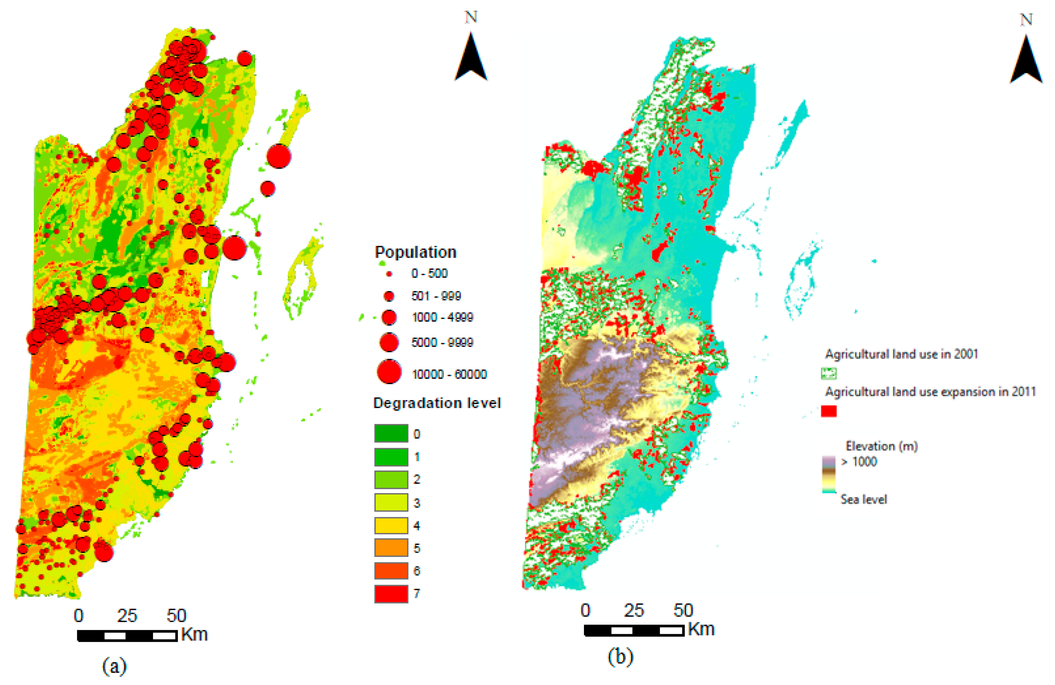
The data generally indicate that fragmentation has affected the ecosystems, especially those in the Orange Walk and Corozal Districts. The expansion of agricultural land use and urbanization has likely led to deforestation. In Figure 6a, the land degradation level shows the highest value in the central portion of Belize, which is the largest forest reserve in the country. This high degradation is likely due to illegal logging, slash and burn, and riparian farms [39]. This degradation (Figure 6a), can also be seen as a bio-economic map, of some sort. The decrease in lowland savannas accommodates for agricultural land use expansion. It is also in this area that the country has seen a drastic increase in population and settlement size [35]. Figure 6b depicts the agricultural expansion (red) in the most significant years, 2001 to 2017. AU increased by more than 800 km2, which is quite large considering the small size of Belize. The most expansion has been in the northern districts, where we have so noted the most drastic decrease in lowland savannah.
A countermeasure of the government has been to concentrate on the protected areas in central Belize. It is possible that this countermeasure is responsible for the fall in fragmentation metric rates from the year 2011 to 2017, (insignificant variance which the post hoc tests and the ANOVA indicate). Whether or not the pace of the countermeasure can ensure the sustainability of the natural flora and fauna is another matter. However, based upon the results, it is highly recommended that some extra measures need to be put in place in addition to the existing, to mitigate the current effects of urbanization and population expansion. There is a need to optimize the mitigation measures that can deter further fragmentation of ecosystems in Belize.
Habitat fragmentation has been a global problem that has been of imperative focus for the conservation and preservation of flora and fauna. As population, urbanization, and agricultural farming increase, they cause biological stress on existing ecosystems, as has been the case in Belize. Landscape metrics were developed to understand and analyze the interaction and response of natural habitats to environmental stress. These metrics offer quick and easy markers that are descriptive of the conditions of a habitat and its biological composition. This study aimed to explain the changes of three Belizean ecosystems using landscape metrics as they are pressed by anthropogenic expansion. These were some of the findings of the study:
- The total area of agricultural uses increased by 14.37% in just 10 years. Overall, there has been an increase of more than 800 km2 in agricultural lands between the study years 2001 and 2011.
- The total area of mangrove and the littoral forest seemed unaffected, as is indicated by the constant CA value. However, the number of patches increased by 284%, which shows that fragmentation can occur irrespective of the total landscape area.
- The changes in ED between years showed a reduction in the heterogeneity of the landscapes, especially for lowland savannahs in the northern part of Belize, which coincides with the agricultural expansion in that area for the cultivation of sugar cane. The MSI also displayed similar behavior, showing that the increasing ED also increased the complexity of the patch shapes, which is indicative of habitat fragmentation.
- The AWMSI values of the AU decreased during the study period. This indicates that although agriculture has been expanding, it is possible that a dominating percentage of this expansion maybe unplanned and informal. This result coincided with the results of ED from AU.
- The MPS for all biotic landscapes decreased, showing that the biota has been fragmented and degraded. The decrease in average patch size ranged from 4.3% to 1182% indicating a massive increase in fragmentation in just 10 years. This was also observed graphically in the land degradation map overlapped with population size and dispersion.
There were also several limitations in this study that could have improved the quality of the results. These limitations also reflect areas where future studies can be improved. Only five landscape classes were used, which limited the analysis of the response of ecosystems to habitat fragmentation in Belize. Moreover, only six landscape metrics were used. These metrics mainly focused on patch shape, area, and distance from edge. However, there are several other types of landscape metric that can provide additional information such as variability, diversity, contagion and interspersion metrics such as those in [40]. Another limitation is that due to the available data, the study period was quite short. As the study stands, there is only a gap of 16 years from the first ecosystem study to the most recent, 2017. It is advisable that a larger time span is used in the future study for analyzing and revealing the habitat variation over times in Belize.
Author Contributions
Conceptualization, B.F. and K.-T.H.; methodology, B.F. and K.-T.H.; software, G.O.A.; formal analysis, B.F.; resources, G.O.A.; data curation, B.F. and G.O.A.; writing—original draft preparation, B.F. and K.-T.H; writing—review and editing, K.-T.H.; visualization, B.F. and G.O.A.; supervision, K.-T.H.; All authors have read and agreed to the published version of the manuscript.
Funding
This research received funding from the Ministry of Science and Technology, Taiwan under project No. MOST107-2221-E-002-049-MY2 to make the publishing of this article possible.
Conflicts of Interest
The authors declare no conflict of interest.
Appendix A

Table A1.
Patch Analyst simulation results for wetlands (WL), urban (URB), mangrove and littoral forest (MLF), lowland savanna (LS), and agricultural use (AU) for the year 2001, 2011, and 2017 in classes AWMSI, MSI, ED, MPS, NUMP, and CA.
Table A1.
Patch Analyst simulation results for wetlands (WL), urban (URB), mangrove and littoral forest (MLF), lowland savanna (LS), and agricultural use (AU) for the year 2001, 2011, and 2017 in classes AWMSI, MSI, ED, MPS, NUMP, and CA.
| Class | 2001 | ||||
| WL | URB | MLF | LS | AU | |
| AWMSI | 2.67 | 1.78 | 2.50 | 2.68 | 4.54 |
| MSI | 1.86 | 1.68 | 1.93 | 1.81 | 1.87 |
| ED | 0.54 | 0.14 | 1.59 | 1.22 | 2.35 |
| MPS | 443.34 | 259.81 | 253.96 | 1912.90 | 1,718 |
| NUMP | 95.00 | 39.00 | 370.00 | 102.00 | 208 |
| CA | 42,117 | 10,132 | 93,965 | 195,116.00 | 357,463 |
| Class | 2011 | ||||
| AWMSI | 4.07 | 1.88 | 2.64 | 3.98 | 7.39 |
| MSI | 1.82 | 1.54 | 1.84 | 2.16 | 1.82 |
| ED | 0.84 | 0.24 | 0.87 | 1.67 | 1.50 |
| MPS | 143.18 | 92.53 | 101.21 | 161.80 | 1,068 |
| NUMP | 716.00 | 298.00 | 922.00 | 1080.00 | 415 |
| CA | 102,518 | 27,574 | 93,312 | 174,746 | 443,317 |
| Class | 2017 | ||||
| AWMSI | 4.45 | 2.35 | 3.07 | 3.77 | 8.45 |
| MSI | 1.93 | 1.79 | 2.03 | 2.11 | 1.81 |
| ED | 0.62 | 0.30 | 0.53 | 1.66 | 1.92 |
| MPS | 137.32 | 78.86 | 81.17 | 295.26 | 683.37 |
| NUMP | 565 | 335 | 1052 | 1151 | 684 |
| CA | 77,588 | 26,420 | 85,394 | 339,846 | 467,422 |
References
- Michigan Forests Forever Teachers Guide. Process of landscape fragmentation. In Michigan Forests Forever Teachers Guide; clark_figure3_ksm.jpg, Ed.; Nature Education: Michigan, MI, USA, 2010; Available online: www.nature.com/ (accessed on 7 May 2019).
- Fahrig, L. How much habitat is enough? Biol. Conserv. 2001, 100, 65–74. [Google Scholar] [CrossRef]
- Miller, K.; Brennan, L.; Perotto-Baldivieso, H.; Hernández, F.; Grahmann, E.; Okay, A.; Wu, X.; Peterson, M.; Hannusch, H.; Mata, J.; et al. Correlates of habitat fragmentation and northern bobwhite abundance in the gulf prairie landscape conservation cooperative. J. Fish Wildl. Manag. 2019, 10, 3–18, e1944-1687X. [Google Scholar] [CrossRef] [Green Version]
- Jackson, S.T.; Hobbs, R.J. Ecological restoration in the light of ecological history. Science (N. Y.) 2009, 325, 567–569. [Google Scholar] [CrossRef] [PubMed] [Green Version]
- Hanski, I. Habitat loss, the dynamics of biodiversity, and a perspective on conservation. Ambio 2011, 40, 248–255. [Google Scholar] [CrossRef] [Green Version]
- Bascompte, J.; Sole, R.V. Habitat fragmentation and extinction thresholds in spatially explicit models. J. Anim. Ecol. 1996, 65, 465–473. [Google Scholar] [CrossRef]
- Donovan, T.M.; Flather, C.H. Relationships among north american songbird trends, habitat fragmentation, and landscape occupancy. Ecol. Appl. 2002, 12, 364–374. [Google Scholar]
- Pimm, S.L.; Jenkins, C.N.; Abell, R.; Brooks, T.M.; Gittleman, J.L.; Joppa, L.N.; Raven, P.H.; Roberts, C.M.; Sexton, J.O. The biodiversity of species and their rates of extinction, distribution, and protection. Science (N. Y.) 2014, 344, 1246752. [Google Scholar] [CrossRef]
- Wang, X.; Blanchet, F.G.; Koper, N. Measuring habitat fragmentation: An evaluation of landscape pattern metrics. Methods Ecol. Evol. 2014, 5, 634–646. [Google Scholar] [CrossRef]
- Fu, B.-J.; Hu, C.-X.; Chen, L.-D.; Honnay, O.; Gulinck, H. Evaluating change in agricultural landscape pattern between 1980 and 2000 in the loess hilly region of ansai county, china. Agric. Ecosyst. Environ. 2006, 114, 387–396. [Google Scholar] [CrossRef]
- O’Neill, R.V.; Krummel, J.R.; Gardner, R.H.; Sugihara, G.; Jackson, B.; DeAngelis, D.L.; Milne, B.T.; Turner, M.G.; Zygmunt, B.; Christensen, S.W.; et al. Indices of landscape pattern. Landsc. Ecol. 1988, 1, 153–162. [Google Scholar] [CrossRef]
- Luck, M.; Wu, J. A gradient analysis of urban landscape pattern: A case study from the phoenix metropolitan region, arizona, USA. Landsc. Ecol. 2002, 17, 327–339. [Google Scholar] [CrossRef]
- Ramachandra, T.V.; Bharath, H.A.; Sreekantha, S. Spatial metrics based landscape structure and dynamics assessment for an emerging indian megalopolis. Int. J. Adv. Res. Artif. Intell. 2012, 1, 48–57. [Google Scholar]
- Uuemaa, E.; Mander, Ü.; Marja, R. Trends in the use of landscape spatial metrics as landscape indicators: A review. Ecol. Indic. 2013, 28, 100–106. [Google Scholar] [CrossRef]
- Ewers, R.M.; Didham, R.K. Confounding factors in the detection of species responses to habitat fragmentation. Biol. Rev. Camb. Philos. Soc. 2006, 81, 117–142. [Google Scholar] [CrossRef] [PubMed]
- Pimm, S.; Askins, R. Forest losses predict bird extinctions in Eastern North-America. Proc. Natl. Acad. Sci. USA 1995, 92, 9343–9347. [Google Scholar] [CrossRef] [PubMed] [Green Version]
- Didham, R.K. Ecological consequences of habitat fragmentation. In Els; John Wiley & Sons, Ltd.: Perth, WA, Australia, 2001. [Google Scholar]
- Cherrington, E.; Ek, E.; Cho, P.; Howell, B.F.; Hernández Sandoval, B.; Anderson, E.; Flores, A.; Garcia, B.C.; Sempris, E.; Irwin, D. Forest Cover and Deforestation in Belize: 1980–2010; SERVIR-Mesoamerica: Panama City, Panama, 2010. [Google Scholar]
- Meerman, J.C.; Sabido, W. Biodiversity in Belize—Ecosystem Map. Available online: http://biological-diversity.info/Ecosystems.htm (accessed on 12 March 2018).
- Tilman, D.; Clark, M.; Williams, D.R.; Kimmel, K.; Polasky, S.; Packer, C. Future threats to biodiversity and pathways to their prevention. Nature 2017, 546, 73. [Google Scholar] [CrossRef]
- Day, M. Resource use in the tropical karstlands of central belize. Environ. Geol. 1993, 21, 122–128. [Google Scholar] [CrossRef]
- Folkard-Tapp, H. Deforestation in belize-what, where and why. bioRxiv 2020. [Google Scholar] [CrossRef]
- UNEP. Protected Area Profile for Belize from the World Database of Protected Areas, March 2018 ed.; Protected Plant: Cambridge, UK, 2018.
- Vogelmann, J.E. Assessment of forest fragmentation in southern new england using remote sensing and geographic information systems technology. Conserv. Biol. 1995, 9, 439–449. [Google Scholar] [CrossRef]
- Schüepp, C. Effects of Habitat Fragmentation and Disturbance on Biodiversity and Ecosystem Functions; Universität Bern: Bern, Switzerland; BORIS: Bern Open Repository and Information System: Bern, Switzerland, 2014. [Google Scholar]
- Meerman, J.; Clabaugh, J. Biodiversity and Environmental Resource Data System of Belize; BERDS: Cayo, Belize, 2017. [Google Scholar]
- CHARIM. Belize 90m bare earth dem. In Caribbean Handbook on Risk Information Management GeoNode, 11th ed.; CHARIM: Enschede, The Netherlands, 2016. [Google Scholar]
- Rempel, R.S.; Kaukinen, D.; Carr, A.P. Patch Analyst and Patch Grid, 5.2; Center for Northern Forest Ecosystem Research, Ontario Ministry of Natural Resources: Thunder Bay, ON, Canada, 2012.
- ESRI. Arcgis Desktop; Release 10.1; Environmental Systems Research Institute: Redlands, CA, USA, 2013. [Google Scholar]
- Turner, M.G.; Gardner, R.H. Landscape Ecology in Theory and Practice: Pattern and Process, 2nd ed.; Springer: New York, NY, USA, 2015; p. 482. [Google Scholar]
- Peng, J.; Wang, Y.L.; Zhang, Y.; Wu, J.S.; Li, W.F.; Li, Y. Evaluating the effectiveness of landscape metrics in quantifying spatial patterns. Ecol. Indic. 2010, 10, 217–223. [Google Scholar] [CrossRef]
- McGarigal, K.; J Marks, B. Fragstats—Spatial Pattern Analysis Program for Quantifying Landscape Structure; University of Massachusetts: Amherst, MA, USA, 1995. [Google Scholar]
- Choi, J.; Lee, S.; Ji, S.; Jeong, J.-C.; Lee, P. Landscape analysis to assess the impact of development projects on forests. Sustainability 2016, 8, 1012. [Google Scholar] [CrossRef] [Green Version]
- Wiedmaier, B. The Sage Encyclopedia of Communication Research Methods; SAGE Publications: Thousand Oaks, CA, USA, 2017. [Google Scholar]
- Ergen, M. Relationship between population and agricultural land in amasya. In Urban Agriculture; IntechOpen: Cairo, Egypt, 2016. [Google Scholar]
- McGarigal, K.; Cushman, S.A.; Neel, M.; Ene, E. Fragstats; University of Massachusetts: Amherst, MA, USA, 2002. [Google Scholar]
- Daye, D.D.; Healey, J.R. Impacts of land-use change on sacred forests at the landscape scale. Glob. Ecol. Conserv. 2015, 3, 349–358. [Google Scholar] [CrossRef] [Green Version]
- Kowe, P.; Pedzisai, E.; Gumindoga, W.; Rwasoka, D.T. An analysis of changes in the urban landscape composition and configuration in the sancaktepe district of istanbul metropolitan city, turkey using landscape metrics and satellite data. Geocarto Int. 2014, 30, 1–14. [Google Scholar] [CrossRef]
- Young, C.A. Belize’s ecosystems: Threats and challenges to conservation in belize. Trop. Conserv. Sci. 2008, 1, 18–33. [Google Scholar] [CrossRef] [Green Version]
- Monmany, A.C.; Yu, M.; Restrepo, C.; Zimmerman, J.K. How are landscape complexity and vegetation structure related across an agricultural frontier in the subtropical chaco, nw argentina? J. Arid Environ. 2015, 123, 12–20. [Google Scholar] [CrossRef]
Figure 1.
Illustration of the process of landscape fragmentation. The process of fragmentation can be summarized in 4 phases: (a) perforation, which sees initial small openings; (b) dissection, illustrates larger intrusions of change, often along with physical features; (c) dissipation, which is the spread and coalescing of alteration, and eventually, (d) shrinkage, which results in the reduction in patch size and attrition [1].

Figure 2.
Widely-held generalizations of how species in ecosystems react to habitat fragmentation. The five main components of the spatial context of habitat fragments are seen in conjunction with species loss. The predictions are derived from studies in fragmentation effects [17].
Figure 2.
Widely-held generalizations of how species in ecosystems react to habitat fragmentation. The five main components of the spatial context of habitat fragments are seen in conjunction with species loss. The predictions are derived from studies in fragmentation effects [17].

Figure 3.
Ecological and political map of Belize in 2011 that illustrates the 5 landscapes that will be the focus of this study [19].
Figure 3.
Ecological and political map of Belize in 2011 that illustrates the 5 landscapes that will be the focus of this study [19].

Figure 4.
(Left) Landscape of the forest cover in 1986; (Right) landscape of the remaining forest in 2018.
Figure 4.
(Left) Landscape of the forest cover in 1986; (Right) landscape of the remaining forest in 2018.

Figure 5.
Landscape metrics variability in number of patches (a), area-weighted mean shape index (b), mean shape index (c), edge density (d), mean patch size (e), and class area (f) in the years 2001, 2011, 2017. The classes are AU—agricultural use, LS—lowland savanna, MLF—mangrove and littoral forest, URB—urban, and WL—wetlands.

Figure 6.
(a) A map of land degradation coupled with settlements and population size as they are drivers to fragmentation. Larger circles indicate larger population sizes, and the coloration of degradation is from green to red-green (0–1) being least degraded and red (7) meaning most degraded; (b) agricultural land expansion from 2001 up to 2017. The total area of the expansion was approximately 858.54 km2 [26].

Table 1.
One-way ANOVA of the NUMP for each land scape metric class for the years 2001, 2011, and 2017.
Table 1.
One-way ANOVA of the NUMP for each land scape metric class for the years 2001, 2011, and 2017.
| Ecosystem/Class | Patch Number (NUMP) | Source of Variation | p-Value | Inference | ||
|---|---|---|---|---|---|---|
| Groups | Between years/Groups | 0.0120 | Significant | |||
| 2001 | 2011 | 2017 | ||||
| Wetlands (WL) | 95 | 716 | 565 | |||
| Urban (URB) | 39 | 298 | 335 | |||
| Mangroves and Littoral Forests (MLF) | 370 | 922 | 1052 | |||
| Lowland savanna (LS) | 102 | 1080 | 1151 | |||
| Agricultural use (AU) | 208 | 415 | 684 | |||
Note: The result is significant at p ≤ 0.05.
Table 2.
Post-hoc tests of number of patches (NUMP) for all 3 years.
| Group Pair | Inference | |
|---|---|---|
| Tukey HSD Test | 2001 vs. 2011 | significant |
| 2001 vs. 2017 | significant | |
| 2011 vs. 2017 | insignificant | |
| Scheffé Multiple Comparison | 2001 vs. 2011 | significant |
| 2001 vs. 2017 | significant | |
| 2011 vs. 2017 | insignificant |
Note: The result is significant at p ≤ 0.05.
© 2020 by the authors. Licensee MDPI, Basel, Switzerland. This article is an open access article distributed under the terms and conditions of the Creative Commons Attribution (CC BY) license (http://creativecommons.org/licenses/by/4.0/).
Share and Cite
MDPI and ACS Style
Flowers, B.; Huang, K.-T.; Aldana, G.O. Analysis of the Habitat Fragmentation of Ecosystems in Belize Using Landscape Metrics. Sustainability 2020, 12, 3024. https://0-doi-org.brum.beds.ac.uk/10.3390/su12073024
AMA Style
Flowers B, Huang K-T, Aldana GO. Analysis of the Habitat Fragmentation of Ecosystems in Belize Using Landscape Metrics. Sustainability. 2020; 12(7):3024. https://0-doi-org.brum.beds.ac.uk/10.3390/su12073024
Chicago/Turabian StyleFlowers, Bryon, Kuo-Tsang Huang, and Gerardo O. Aldana. 2020. "Analysis of the Habitat Fragmentation of Ecosystems in Belize Using Landscape Metrics" Sustainability 12, no. 7: 3024. https://0-doi-org.brum.beds.ac.uk/10.3390/su12073024
Note that from the first issue of 2016, this journal uses article numbers instead of page numbers. See further details here.