A System Dynamics Model of Supply-Side Issues Influencing Beef Consumption in Nigeria


1
Department of Agricultural Economics, University of Ibadan, Ibadan 200284, Nigeria
2
Department of Civil Engineering, George Fox University, Newberg, OR 97132, USA
3
MM-Five GmbH—Mobility, Futures, Innovation, Economics, Bahnhofstr. 46, 76137 Karlsruhe, Germany
*
Authors to whom correspondence should be addressed.
Sustainability 2020, 12(8), 3241; https://0-doi-org.brum.beds.ac.uk/10.3390/su12083241
Submission received: 31 January 2020
/
Revised: 10 April 2020
/
Accepted: 13 April 2020
/
Published: 16 April 2020
(This article belongs to the Special Issue Global Engineering and Sustainable Development)
Abstract
:The per capita consumption of beef in Nigeria is reducing amidst a rising population that is dependent on beef as a major source of animal protein. In this paper, a system dynamics (SD) model was developed with the aim of testing exploratory policies aimed at reversing this trend. The simulations of various policy tests showed that, of all the policies tested, having a higher carcass yield seems to be the most efficient solution, but its feasibility faces some steep biological and ecological challenges. However, a combination of policies that cuts across the land–cattle–market nexus is necessary to obtain a consumption level that almost meets the World Health Organization (WHO) standards for recommended animal protein intake. Complex inter-linked systems, like beef production and consumption, require a systemic approach that considers dynamic feedback to avoid fixes that fail or shift the burden when making policy decisions.
1. Introduction
Low levels of animal protein intake among Nigerians result from a low level of beef consumption per capita (BCPC). This low level of beef consumption is strongly linked to malnutrition, especially among children in developing countries [1,2,3,4]). Several studies recommend a supply-side approach to meet consumption needs, such as increasing herd size, livestock density and supply chain efficiency, while noting the negative impacts on land and environment [5,6,7,8,9]. The emerging issues of sustainable food systems, and the effect of climate change on increased livestock production, as studied by Herrero and Thornton [10] and Nardone et al. [11], have led to a call for more sustainable and ethical beef consumption [12,13,14]. According to the Food and Agriculture Organization of the United Nations (FAO), the total stock of cattle and total annual cattle slaughtered in Nigeria increased from 13.9 million head and 144,000 head in 1990, respectively, to 20 million head and 321,000 head in 2017, respectively. However, the carcass yield of indigenous cattle reduced from 141 kg/animal in 1991 to 116 kg/animal in 2017 [15].
Beef consumption is inherently dependent on several interlinked and dynamic systems (e.g., land resource, cattle production and the beef market), with feedback from multiple dependent variables instead of a single, static, linear system [16,17,18,19]. We posit that policies that consider these systemic and dynamic multi-variable feedback interactions will yield the greatest overall increase in beef supply and consequently consumption. One such methodology for modeling the interaction between system and subsystem factors is System Dynamics (SD) modeling. SD modeling provides a means to conceptualize and simulate dynamic interaction and feedbacks between endogenous and exogenous factors observed in the sector, and offers insight into key leverage points in order to influence policy-making and action to optimize impact [20]. Here, we apply SD modeling to understand the key structural drivers of Nigerian beef consumption. The overarching questions that this research seeks to address are: (i) what structure is responsible for low beef consumption among Nigerians? and (ii) how might beef consumption be increased? The related objectives that guided this research are, therefore: (i) to determine the key drivers for Nigerian beef consumption levels, and (ii) to explore how these drivers interact as a system and thus propose potentially effective ways to improve beef consumption levels.
To achieve our research objectives, we first developed a causal loop diagram (CLD) to model the interaction of drivers hypothesized to influence beef consumption in Nigeria. The CLD was based on an intellectual model skewed towards modeling consumption from a market supply-based standpoint, without recourse to other socioeconomic characteristics aside from income, which influences consumer demand. This CLD was then used to build a stock and flow (SF) SD model to simulate various policy solutions and identify leverage points for recommended interventions The ensuing models and diagrams are particularly applicable to the typical Nigerian livestock system and are potentially generalizable for free-grazing systems, a pasture-based production system practiced in communal grazing lands that is constrained by seasonality in feed availability following rainfall and typical of most other African countries.
It is important to note that the model and policy tests ran using the model are intended to provide “exploratory” analyses to help determine which policies are worth assessing in future research. Additionally, modifications would need to be made to the model to fit semi-intensive or farm-style livestock systems. Semi-intensive livestock systems are partly confined systems where cattle are allowed to graze freely or under paddocking with the provision of feed supplements and constrained by seasonal changes in water and pasture availability. Farm systems are intensive systems with a high level of feed and resource management that can be constrained by high feed and veterinary service costs due to the risk of disease spread from the close confinement of cattle.
The following sections start with a review of protein intake and beef consumption levels in Nigeria and then a review of the literature on livestock sector dynamics and their limitations. We then discuss the challenges facing the beef industry in Nigeria and detail how this study aims to address these challenges with the results of SD-based policy analysis. Finally, based on the findings of the study, we offer recommendations for policy and practice in the Nigerian livestock industry to improve BCPC in Nigeria and identify potential areas for future research to expand upon these findings. To encourage model replication, this paper utilizes a narrative method to portray the model description and building process. To this end, a link is provided in Appendix A to access the Stella Architect model, and all assumptions and the underlying mathematical equations used are shown in Appendix B.
2. Literature Review
In this section, we summarize the literature that focuses on (i) protein consumption in Nigeria, (ii) the broader dynamic drivers of beef production, (iii) the past application of system dynamics modeling to elucidate and understand these drivers, and (iv) the challenges specific to the Nigerian livestock context. Based on this summary, we elucidate gaps in knowledge that we propose to address within our study.
2.1. Protein Consumption in Nigeria
The Recommended Dietary Allowance (RDA) for protein consumption has been estimated by the WHO at 0.8 g/kg/day [21]. This amounts to 56 g/capita/day or 20.4 kg/capita/year for an adult weighing 63.5 kg. It is important to note that the minimum recommended level, or “recommended intake”, is not necessarily the ideal level of protein intake, but the one below which health conditions deteriorate. For instance, the FAO recommendation for daily protein consumption is 60 g per person, of which 30 g is expected to be from an animal source. Data from the FAO shows that the average per capita protein intake for Nigeria in 2013 was 63.8 g, of which only 10 g came from animal sources. This is in contrast with figures from developed countries, where the average per capita protein intake was over 80 g, with more than 55 g of animal protein [22].
It has been estimated that the daily minimum crude protein requirement of an adult in Nigeria varies between 65 g and 85 g per person. However, it is recommended that 30 g of this minimum requirement should be obtained from animal products [23] in order to enrich the dietary quality with other nutrients and amino acids obtained from other sources. A review of the data on food supplies available for consumption in different countries shows that the per capita protein intakes (especially from animal sources in developing countries) is directly and indirectly related to various health-related issues like stunted growth, low strength and acute protein malnutrition, especially among children. Not only is the total protein supply deficient in these contexts but the quality of dietary protein available is inferior to that consumed in developed countries [24]. Figures on the average crude protein consumption per day in Nigeria fall short of the recommendations of the FAO [25]. In Nigeria, a few varieties of plant, including cowpea, groundnut and millet, supply most of the dietary protein consumed [26]. The low level of animal protein consumption in Nigeria, as reported by the FAO, revealed that the diet of an average Nigerian contains 33 percent less than the recommended requirement, showing that the average Nigerian diet is deficient of other basic nutrients like iron, lysine and niacin [21]. These data for Nigeria also showed a 6.7% rate of undernourishment in 2013, which rose to 11.5% in 2017 [15]. Furthermore, income level distribution can serve as a proxy for protein consumption (because of high meat prices), analyzed using the Gini coefficient [27,28,29,30], even as Nigeria’s BCPC aligns with this proxy.
2.2. Modeling Livestock Sector Dynamics
SD models have been used to evaluate livestock production systems [31,32,33,34] as well as the sustainability of these systems [35]. In addition, SD models of beef production systems, although high level in nature, have been built for various purposes. These models mainly provide isolated views of the larger complex system, and not of the drivers of, and patterns regarding, beef consumption. For instance, in the study by Kahn and Lehrer [36], the authors focus on the issues related to the reproductive performance of cows [36]. A study by Sobrosa Neto et al. offered an integrative approach to a sustainable beef cattle production model that was limited to the water, energy and food (WEF) nexus, while neglecting the pressure on land as a resource [37]. Similarly, Li et al. considered the trade-offs between water, energy, land and food, with an optimized dynamic model being developed for agricultural cropping systems [38]. Pang et al. used a dynamic deterministic approach to model beef cattle production systems. Their model considered economics, herd inventory, nutrient requirement and forage production as sub-models, yet it was only able to evaluate production traits and management strategies on the production system’s efficiency and lacked validation due to the unavailability of a suitable data set [39]. A system dynamics model by Turner et al., considered cattle production dynamics based on financial incentives for a farm system, and served as a decision-making tool at the farm level [40]. However, their modeling concept has little application to Nigeria, as Nigerian cattle are mainly free rangers and only very few are kept on farms where the bulls and cows can be separated. In contrast, Ash et al., looked at the production and financial consequences for northern Australian beef farms via several technological changes in nutrient supplement, feed base and carcass yield through genetic modification. This particular study, while addressing productivity issues, was more concerned about the viability of beef enterprises [41].
Through model simulation, Guimarães et al., show that small changes in reproduction and mortality rates can considerably affect goat herd dynamics, as they relate to production outputs and profitability [42]. In a study by Gebre et al., increased body weight in sheep through genetic improvement resulted in a lower herd size requirement for mutton production [43], thereby reducing the pressure on land resources. The simulation from the study also demonstrates that breeding for heavier body weight was considerably more profitable than the baseline scenario.
2.3. Challenges Facing the Nigerian Beef Industry
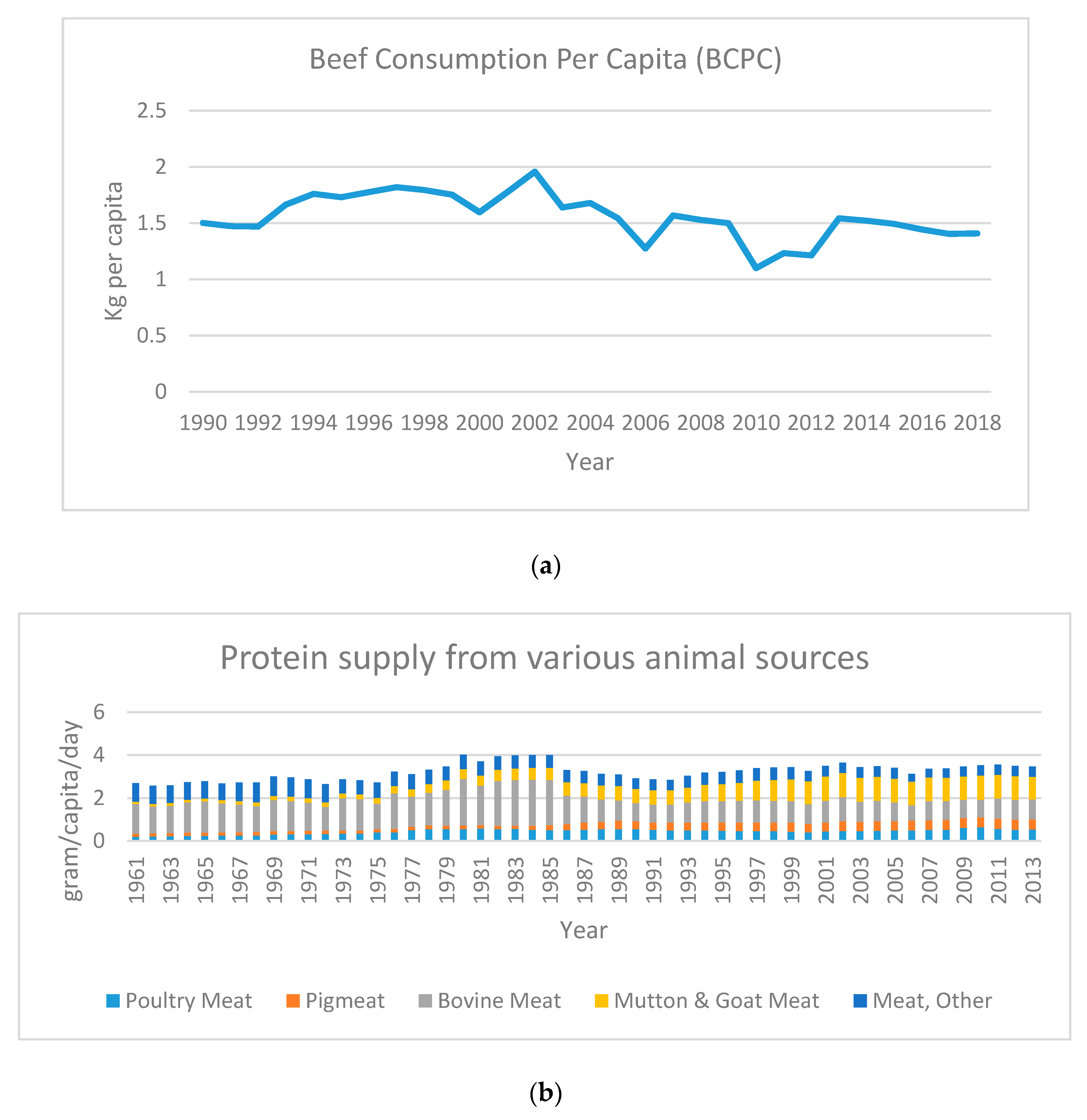
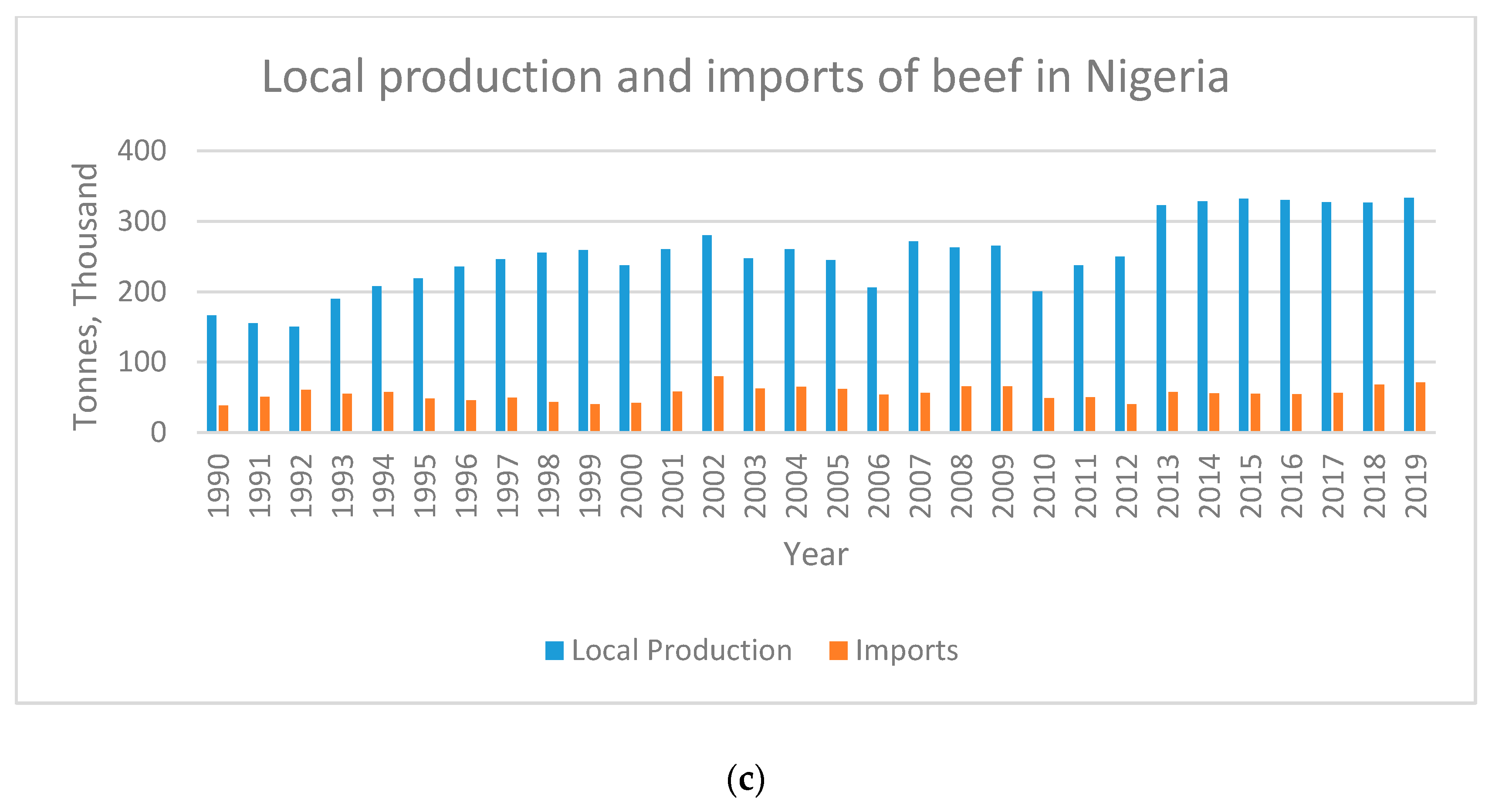
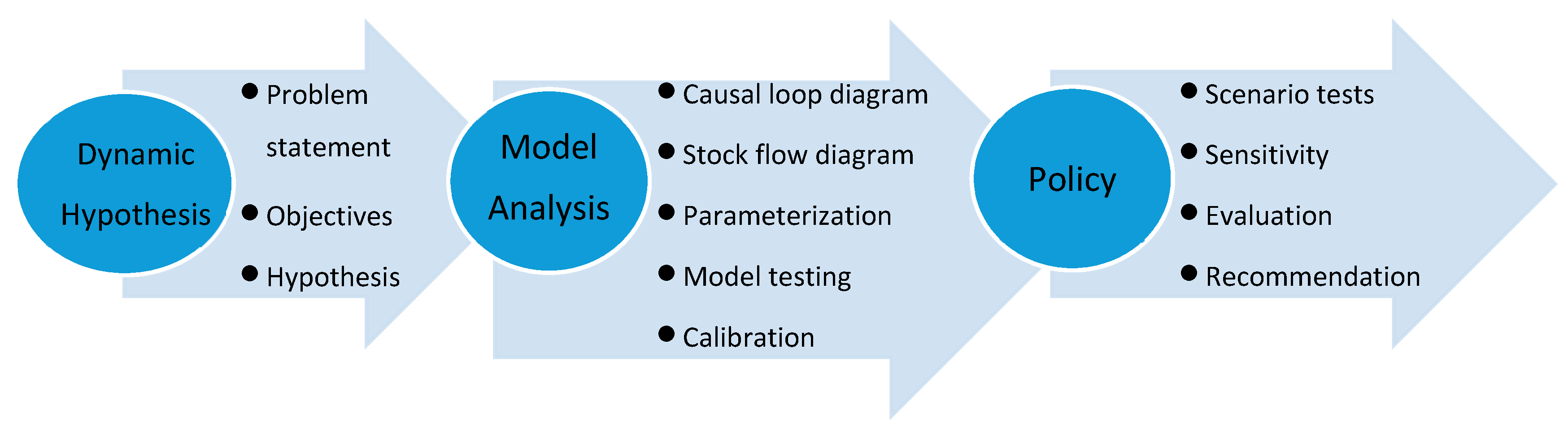
The beef sector in Nigeria has historically been small and slow relative to the growing population [44,45]. Figure 1a show that BCPC has been rising on average from 1993–2013 and since then has been falling with a downward trend from 2004–2018. Figure 1b shows that, although protein supply from cattle is higher than other animal sources, it has been declining over time. This trend in BCPC was used as the reference mode to calibrate the stock and flow SD model used in this study. It has been reported that with Lagos consuming over 8000 cattle daily, along with having a calving rate that is below the consumption rate, the area may suffer scarcity of beef in the future [46]. The livestock industry also plays a significant role in Nigeria’s economy, contributing 5–6% of the country’s total gross domestic product (GDP) and 15–20% of the agricultural GDP [47]. Figure 1c shows the proportion of imported versus local beef production in Nigeria. A rapidly growing population, combined with rising middle-class income, beef supply deficit, currency devaluation, and high transport cost and security challenges in the northeast of the country, have all contributed to Nigeria having the highest cost of beef in Africa. [48]. Concurrently, there is a dearth of cohesive stakeholder interventions in the livestock industry, with no working breeding or herd improvement programs [49]. The problem is further exacerbated by poor infrastructure, with minimal and poor strategic investments in cold storage rooms, processing facilities, and rail and road systems for beef transportation [50]. There is also the challenge of managing natural resources, especially in the face of adverse climatic and environmental conditions [51]. In sum, it is extremely challenging to provide a sustainable supply of beef to meet rising consumption in Nigeria [51,52]. Without a systemic process that leads to understanding the root causes of the problems faced by the beef industry, consumption levels will remain inadequate.
2.4. Point of Departure
The aforementioned literature review points to three gaps: (i) a lack of research that focuses on beef consumption rates, (ii) the need for a model that is fit for purpose for Nigeria’s specific cattle system, and (iii) a need for livestock system models that consider various multi-sector policies to increase BCPC. In addressing these three gaps, our study seeks to develop a deeper understanding of the key drivers of sustained beef consumption through the beef supply system in Nigeria. By modeling the interactions between closely related subsectors within the Nigerian cattle and beef system, we make recommendations to increase beef consumption.
3. Materials and Methods
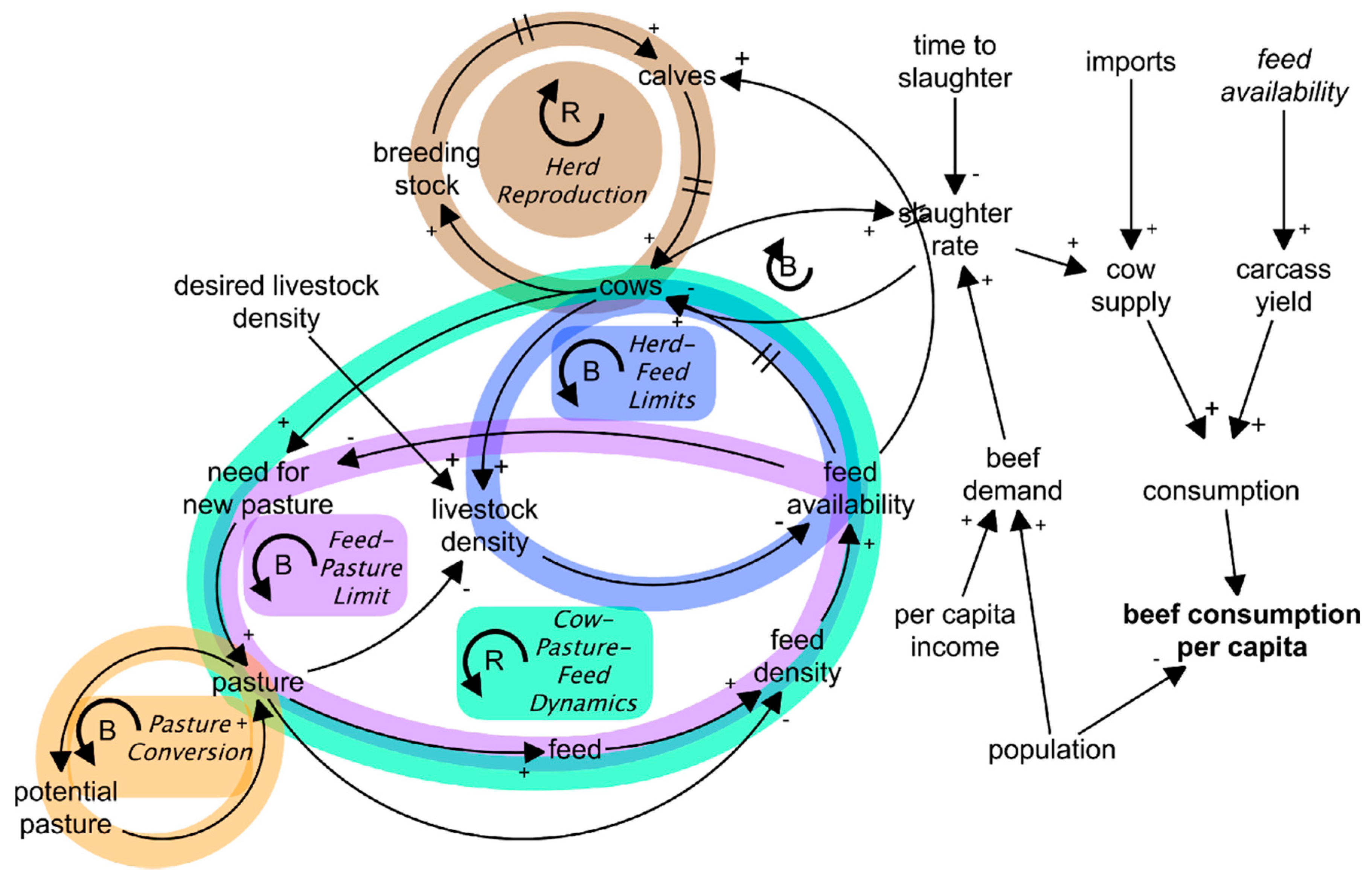
SD model creation began with the development of a causal loop diagram. This CLD qualitatively represented our mental models of system interactions, based on the reviewed literature and from informal interviews with livestock producers. The feedback loops that emerged in the CLD model helped us to develop a more representative and credible model of the real interconnected system, wherein feedback loops drive dynamic model behavior [20,54,55]. In analyzing the CLD, we considered the influence between two variables linked by an arrow bearing a link polarity (“+”: a change in a variable causes a change in the same direction in a variable it is influencing; and “–“: a change in a variable causes a change in the opposite direction in a variable it is influencing). Following the link polarities around a closed feedback loop, it is possible to characterize a loop as reinforcing or balancing by summing the number of negative polarities—where an even sum of negative polarities implies reinforcing, and an odd sum implies balancing. By reasoning through the potential interaction of a several feedback loops, it is possible to hypothesize emergent system behavior, whether growing, decaying or oscillating (involving at minimum two delays). An arrow that is marked with two parallel lines in the middle indicates a causal connection with substantial delays between cause and effect. The CLD offered higher-level consideration and characterization of the feedback loops that drive system behavior, thereafter guiding further analysis and insight through SF diagram-based simulation. Within the SF model, it was then possible to consider policy scenarios that might improve the system behavior of interest, which we define as higher BCPC. The overall process for model development, simulation and testing is presented in Figure 2.
The SF model was set to simulate from the year 1990 to 2030. Secondary, quantitative data for model parameterization and calibration for the Nigerian context was obtained using Knoema [56], a free-to-use public and open data platform from the FAO and the Organization for Economic Cooperation and Development, with data ranging from 1990–2018. The available data informed the model creation, even as suitable historic data on socioeconomic characteristics, as well as other demand-side information, were largely unavailable. The simulation end date was set at 2030, corresponding with the termination date of the Sustainable Development Goals (SDGs). It is assumed that realizing an increased BCPC to the recommended level by this date will contribute to achieving SDG 2: “End hunger, achieve food security and improved nutrition and promote sustainable agriculture” [57]. The model was calibrated using a partial model calibration method [58,59], where key variables in the various modules (model subsystems) were adjusted to fit the trend of real historic data by adjusting constants within the acceptable range. A module-by-module approach was used for calibration. This allowed us to fit each module to its observable trend before linking the subsystems. This process increased the likelihood of the parameter values being close to reality by reducing the degrees of freedom. In addition, it made the overall calibration process easier and gave us a better understanding of the underlying causes of model behavior. Estimates of the parameter values were obtained from a literature review in combination with our best judgement. Time series data used for the calibration of endogenous variables, such as slaughter rate, pasture, herd stock, along with exogenous variables, such as population and per capita GDP, were obtained from international organization sources including the United Nations Conference on Trade and Development (UNCTAD) and the World Bank (see Table A1 in Appendix B).
4. Results and Discussion
This section offers a description of the simulation results, their interpretation, and the recommendations that can be drawn from these results.
4.1. Causal Loop Diagram
The development of the CLD, shown in Figure 3, reveals several balancing and reinforcing feedback loops, which we name on the diagram. The CLD was developed based on our understanding of the system driving beef consumption in Nigeria, and was then iteratively modified after additional insights gained through the completion and simulation of the SF model. The Herd Reproduction loop represents the cattle herd population growth, which is a reinforcing (R) feedback loop. In this loop, having a larger herd size will usually translate into a larger calf population, which in turn leads to an even higher herd size over time. The delay mark indicates that the reproduction and maturation process take significant time and impose a potential oscillatory response in the overall livestock production system. The reinforcing loop (R) Cow-Pasture-Feed Dynamics loop indicates that having a larger herd size will increase the need for new pasture, concurrently increasing pasture for grazing purposes to increase feed. Increasing feed increases the feed density as well as feed availability, providing nourishment for an increasing cattle herd size. The increasing herd size due to growing feed availability is not instantaneous but delayed by maturation time and reproduction time. With adequate feed available, the herd size will increase, thereby further increasing the demand for pasture. The balancing loop (B), Herd-Feed Limits, depicts a structure that counteracts herd size growth. This takes place through the balancing mechanism of desired livestock density. A larger cattle herd size leads to a higher livestock density, which means that the cattle will have less feed to consume per animal, with a concurrent decline of herd size growth. For the Feed-Pasture Limit balancing loop (B), feed availability (together with the herd size) requires an increasing need for new pasture where the pasture is increased through the conversion of new lands (potential pasture). This results in increased feed and feed density, which increases feed availability and thus decreases the need for new pasture. Finally, Pasture Conversion is a balancing loop (B), where an increase in pasture stock leads to a depletion of the potential pasture stock, which ultimately limits further increases in pasture.
While the CLD enables the identification of key drivers of system behavior, it is alone insufficient for evaluating which feedback loop is the most dominant and when. In addition, a CLD does not offer explicit consideration of policies and the measurable effects of these policies. As such, the next step in understanding how system structure drives behavior was to develop a quantitative model (parameterized SF model) to evaluate the loops found in the CLD with numerical values and to test model outputs.
4.2. Stock Flow (SF) Analysis
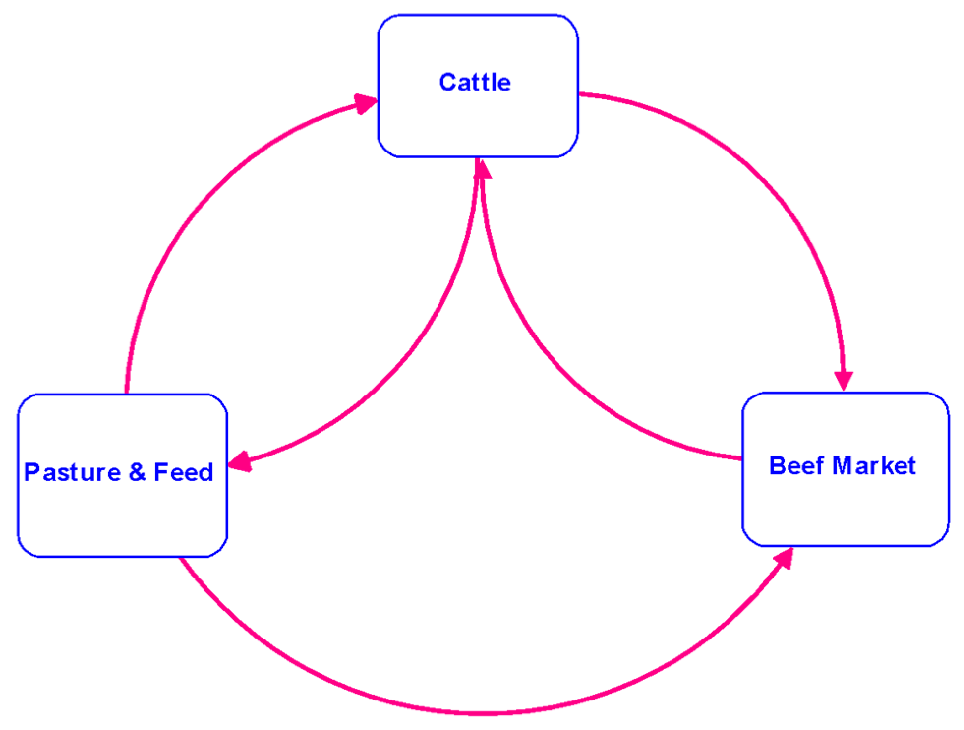
We used Stella Architect modeling software [60] for developing both the CLD and SF models presented here. To offer high-level insight into key model dynamics and to avoid visual clutter, the SF diagram was divided into three interconnected subsystem modules including cattle, pasture/feed and beef market, shown in Figure 4. The top-level module structure necessarily mirrors the overall causal structure hypothesized in the CLD (Figure 3). Figure 4 shows a feedback loop between the Pasture & Feed and Cattle modules, indicating that, as cattle herd size increases, feed from pasture reduces, and vice versa. There is also a feedback loop between the Cattle and Beef market modules: as cattle stock increases, the quantity of beef supplied to the market increases, and the rising demand provides an incentive for higher cattle production. The stock of beef in the beef market is also increased by the effect of available feed on carcass yield (see beef market module for details, Figure 5). The SF structures used within each of the subsystem modules are explained below.
4.2.1. Pasture and Feed Module
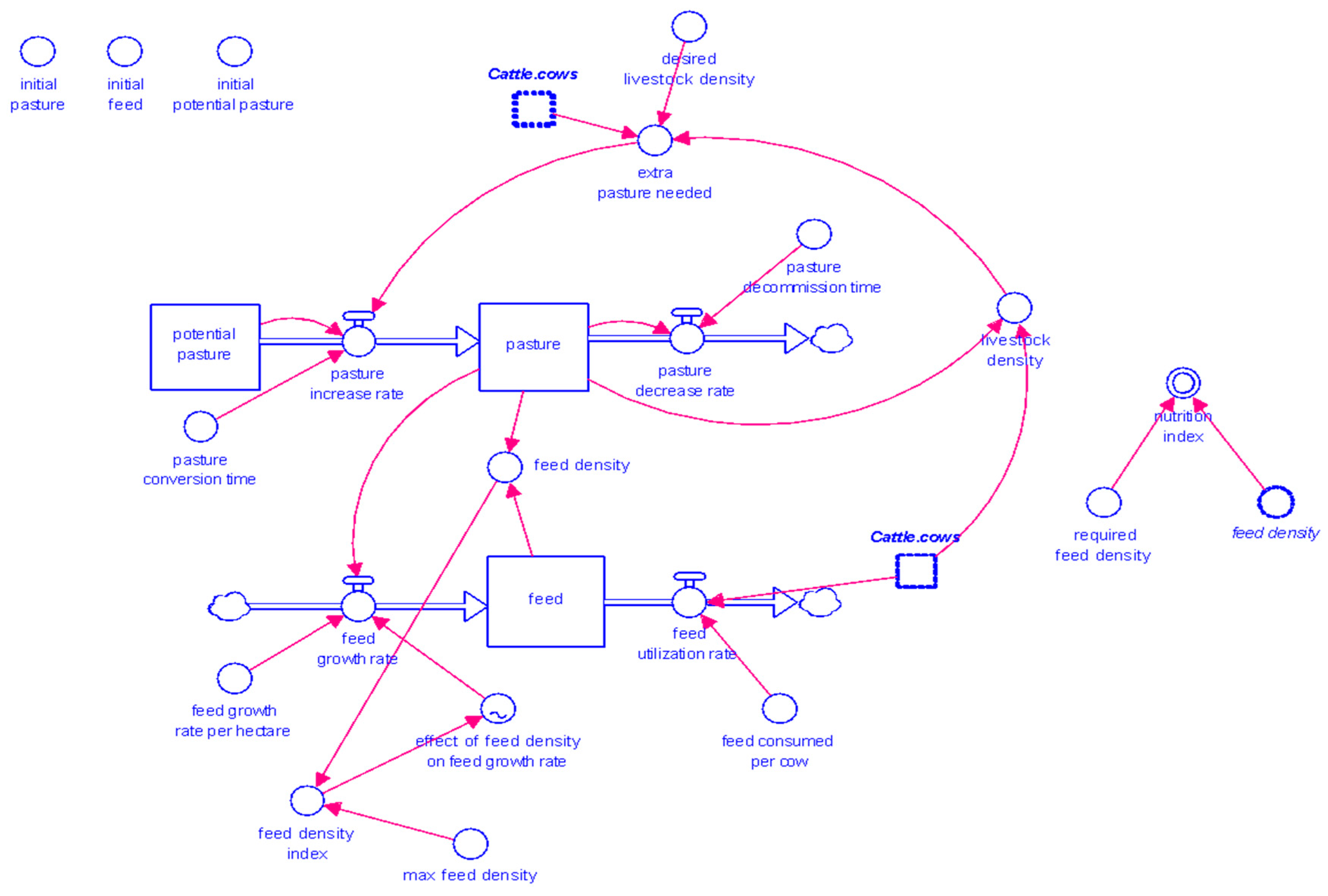
The Pasture & Feed module in the SF model contains three stocks influenced by four flows, which are, in turn, driven by the stocks and converters shown in Figure 5. As Potential Pasture becomes needed for grazing due to increasing cattle herd population, along with the need to maintain a desired livestock density, this land becomes converted to pasture which, over time, is used for other purposes, or left fallow. In 2016, the FAO reported that the Nigerian land that is permanent meadow and pasture is around 30 million hectares, representing 40 percent of the total land available (70 million hectares) for agriculture. [22]. Pasture (in hectares) influences feed (in tons) available, which is influenced by the feed growth rate per hectare of pasture. Feed is depleted through consumption by cattle. The feed density (normalized by dividing it with the required feed density: recommended nutrient intake for cattle) is used to compute the nutrition index, which serves as an indicator of the sufficiency of feed density.
4.2.2. Cattle Module
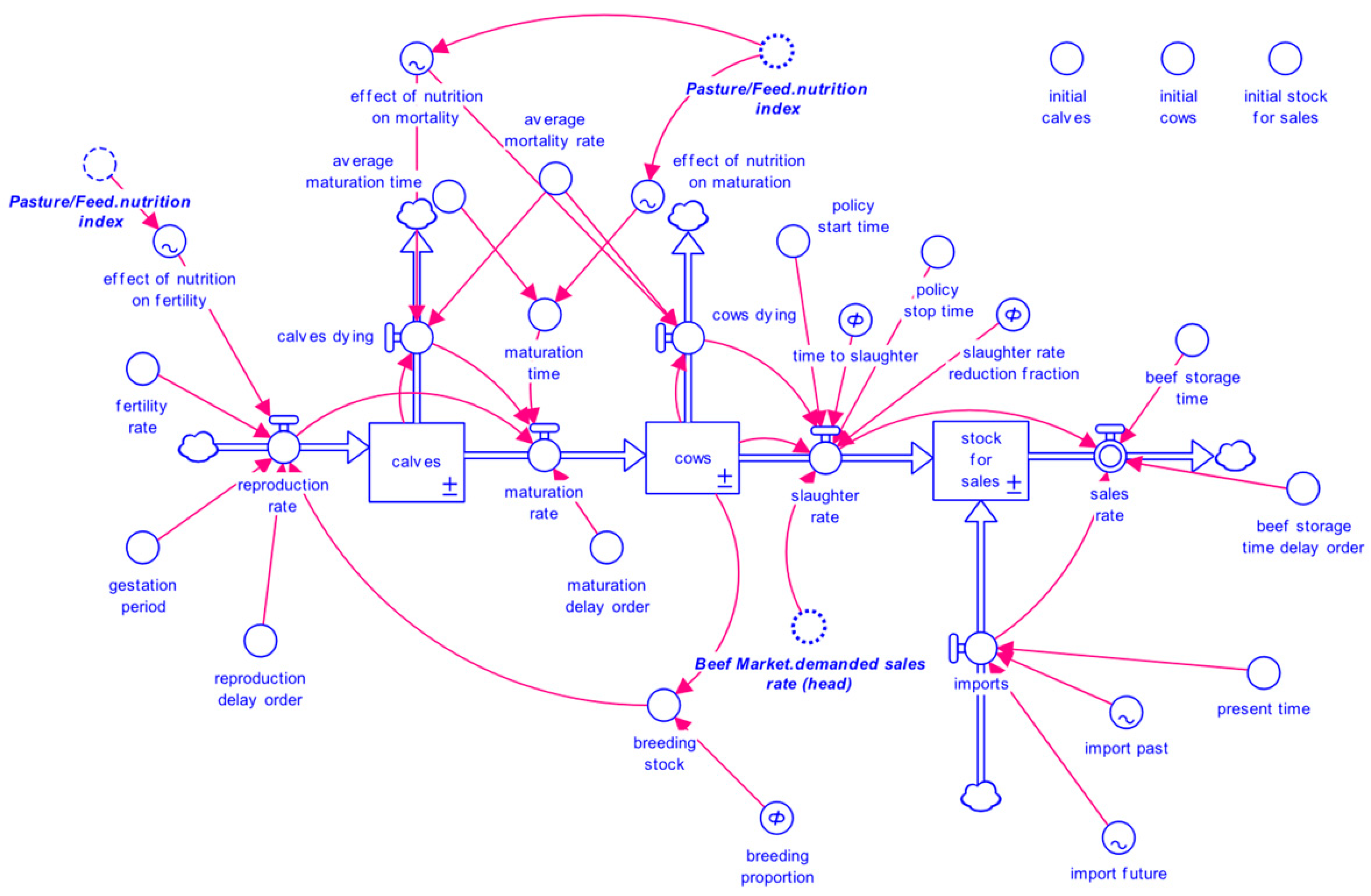
The Cattle module contains the SF model shown in Figure 6. The cattle module is based on a typical aging chain ([20], p. 839) of cattle with calves and cows and includes a terminal flow of sales rate of cows from stock for sales, with all stocks in unit head. The reproduction rate is determined by the breeding stock, fertility rate, gestation period and the effect of nutrition on fertility. The reproduction rate flow increases the calves’ stock, which over time flows out of the system, given the mortality rate, or continues in the system to the cows’ stock through the maturation rate flow. The cows’ stock goes into the stock for sales through the slaughter rate, which is determined by the demanded sales rate from the market sector and time to slaughter. The stock for sales increases via the slaughter rate and imports flow decrease via the sales rate, which is a partially delayed version of the slaughter rate, where beef storage time is the average duration it takes for slaughtered cows to be sold. Besides domestic production, imported beef may also be sold.
4.2.3. Beef Market Module
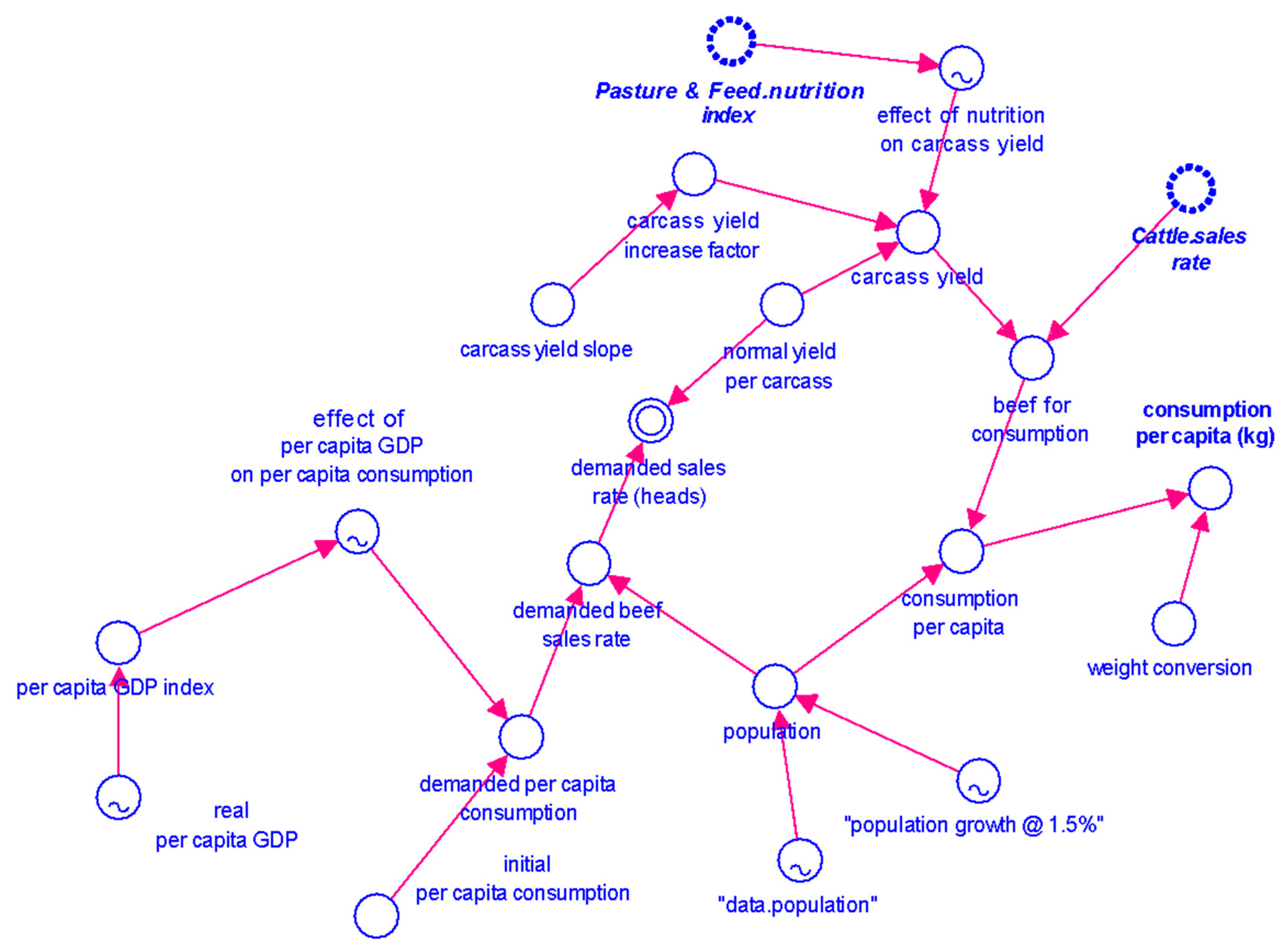
In the Beef Market module (Figure 7), we make use of converters to define the market system and its relationship with BCPC. Real per capita GDP—serving as a proxy for consumer purchasing power as well as an initial per capita consumption—was used to model the demanded per capita consumption. This is because beef is a relatively high-priced food that cannot be bought in desired quantities by people with low sources of income. Population was used to estimate Nigeria’s total demand for beef sales rate by a growing number of consumer. Demanded beef sales rate (tons per year) via carcass yield (carcass yield in this study represents the carcass weight produced per animal head with units in tons/head, as opposed to carcass weight as a percentage of live weight) was converted to demanded sales rate (head per year), a parameter for defining slaughter rate in the Cattle module. The carcass yield, influenced by the effect of nutrition on carcass yield (where better nutrition of cattle leads to an increase in body weight), was used to convert the sales rate in cattle head to total beef consumption in tons. Finally, population and a weight conversion factor to convert tons to kg were used to determine the beef consumption per capita in kg.
4.3. Policy Tests, Analyses and Recommendations
In this section, we perform policy tests and analyses to assess the key drivers of BCPC in Nigeria, and from these analyses propose strategies for policy and practice in order to improve consumption levels. As was previously mentioned, the goal of modeling the drivers of BCPC in Nigeria was to simulate various policies, or “exploratory” scenarios, in order to improve the behavior of the reference mode (historical change in BCPC over time, Figure 1) based on three hypothesized policy schemes. Overall, we aimed to meet the recommended dietary allowance (60 g) for animal protein intake [21] by increasing BCPC by a minimum of three times its current level; thus, the feasibility of the policy assumptions were relaxed. This yields a 7 kg/capita/year beef consumption policy goal to be achieved by 2030.
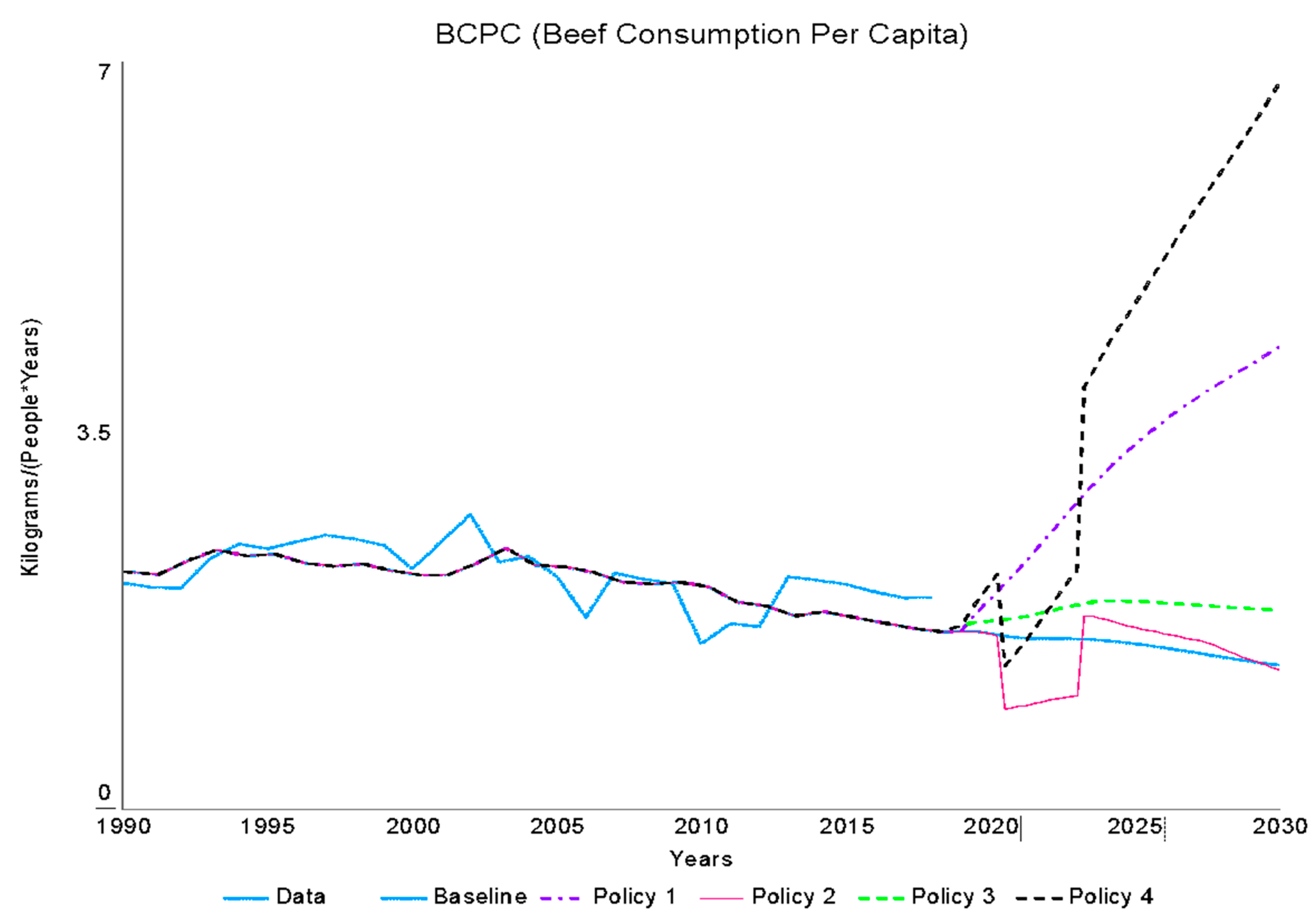
Below we present the four hypothesized policies, each with the potential to increase BCPC. The results can be seen below in Figure 8.
- Policy 1—Improved Feed Growth: improvement in quantity and quality of feed available as a result of higher feed growth rate through the use of practices such as organic manure produced from cattle feces and improved pasture management. Within this policy simulation, we assume that feed growth rate per hectare is increased to a feasible value of 1.3 tons/hectare/year from its current level of 1.05 tons/hectare/year through a pasture improvement plan. This plan could include cultivation of high yielding crops that are easily convertible to nutrients when grazed upon or pasture rotation to reduce the depletion of soil nutrients to promote pasture growth.
- Policy 2—Lower Slaughter Rate: encouraging a larger cows’ stock via the reduction of the slaughter rate for a limited period. Within this policy simulation, slaughter rate reduction was assumed to last for three years (2019–2022). In this policy case, herders will reduce the number of cattle that are sold to the market for slaughter. A sensitivity analysis was carried out on the slaughter rate reduction fraction (the percentage by which the rate of slaughter will be reduced) to determine the value that gives the highest increase in cattle. This analysis yielded a slaughter rate reduction fraction of 0.51 or 51%.
- Policy 3—Higher Carcass Yield: increasing carcass yield via a carcass yield improvement program (parameterized as carcass yield slope), whereby higher-producing beef cattle are bred. A carcass yield slope value of 0.2 would double the carcass yield by 2030 following a constant increase. If this were accomplished, the new carcass yield values in 2030 would be equivalent to the current carcass yield value of developed countries like Germany and the United States of America (see the FAO data). This would be attainable if similar livestock technology and management practices could be used in Nigeria. Such an approach would necessarily require thoughtful consideration of the unique differences between developed countries and Nigeria regarding breed adaptability, feed requirement, utilization and conversion issues, as well as grazing, land and water management, and financial constraints.
- Policy 4—Combined Policies: combined simulation of Policies 1, 2, and 3 to observe desirable and undesirable synergistic effects on the BCPC.
Figure 8 presents a compilation of graphs showing the historic data, the baseline simulation calibrated with these data, and the four policy scenarios that were tested in the model. As the goal of the model was to produce scenarios of BCPC outputs, the policy tests for all scenarios were set to begin from 2018 and run until 2030, with the key output of BCPC in kg/capita/year. The figure shows that there is a good fit between the model’s baseline and historic data runs, thereby increasing the confidence in the model for use in policy tests.
For Policy 1, where available feed is doubled and the feed utilization rate is held constant, we observe that BCPC increases gradually at first and then decreases slightly with a maximum gain of 0.4 kg/capita/y—producing less than a 35% increase on the baseline (“business as usual”) run. For Policy 2, where the slaughter rate was reduced by 51% from 2019 to 2022 and imports were assumed to be held constant, we observe that BCPC takes an initial plunge and thereafter is higher than the baseline scenario, but then decreases and at the end of the run to the same level as the baseline scenario by 2030. Policy 3, where carcass yield is gradually increased to twice its current level by 2030, shows a steady increase in BCPC to more than triple the baseline scenario value in 2030. Finally, for Policy 4, the combination of Policies 1, 2 and 3, we observe a gradual increase in BCPC, due to the carcass yield and feed growth rate policies, and, shortly after, a brief dip due to the slaughter rate policy. We then see a gradual increase during the remaining period of the slaughter rate policy. Immediately after the end of the slaughter rate policy period, we observe a very steep but short-lived rise in BCPC followed by a less steep increase for the remainder of the simulation period. At the end of this simulation run, a beef consumption level at 6.8 kg/cap/y is obtained, which is approximately five times greater than the baseline scenario.
Based on the aforementioned model outputs for the hypothesized policy and leverage points, we provide the following recommendations for policy and practice within the Nigeria livestock sector:
Policy 1—Improved Feed Growth: An increase in the feed stock via a higher feed growth rate per hectare, obtainable through improvement in pasture productivity, can lead to slightly higher BCPC. Alternatively, a higher stock of feed (which also increases the feed available without increasing pasture) could be obtained via a more efficient utilization of feed consumed per cow. In this case, consumption, although decreasing slightly after a modest increase from 2019 to 2024, would be 1.9 kg/capita/y by 2030, as opposed to 1.4 kg/capita/y in the baseline scenario, which is far from the desired goal of 7 kg/capita/y. The analysis of the model indicates that this suboptimal outcome results from a low conversion of feed to carcass yield and a stagnant cattle population.
Policy 2—Lower Slaughter Rate: Increasing cattle herd population through slaughter rate reduction does lead to a higher consumption level when compared to the baseline scenario in 2024; but this increase is short-lived and returns to the baseline level by 2030. This outcome results from a herd size increase early on, only to be discounted by poor nutrition later on, which lowers carcass yield. By summing the area between the Policy 2 and baseline graphs (Figure 8), we find that less beef is consumed overall, far from hitting the policy target of 7 kg/capita/y by 2030.
Policy 3—Higher Carcass Yield: The model simulation shows that carcass yield improvement programs that steadily increase the carcass yield to twice its current level by 2030 could more than triple beef consumption level to 4.3 kg/capita/y by 2030. Despite these potential gains, this still does not achieve the desired consumption level of 7 kg/capita/y. It is important to note that this policy neglects any negative influence on other variables in this model, as all positive gains in BCPC are assumed to be obtained from external efficiencies. This is because such policies would hypothetically be implemented through yield improvement programs that are assumed to be properly funded and managed.
Policy 4—Combined Policies: When all policies are combined, BCPC rises to 6.8 kg/capita/y by 2030, thereby achieving the consumption goal. We see that the slaughter rate policy (Policy 2) causes a dip below the baseline scenario early on, but we get a much higher consumption level in the future than when the slaughter rate policy is excluded from the policy combination. The synergy that exists when the policies are combined shows that such an option is the most preferred for planning strategies to increase BCPC, especially as the resulting benefit of the synergy is higher than the sum of the individual policies. A practical application of such policy combination could follow a process whereby (i) organic fertilizers are applied to pasture, while ensuring that pastures are not totally depleted when grazed upon; (ii) herdsmen decide to reduce mature female cattle sold to market; and (iii) the government and cattle stakeholders establish regional breeding programs that increase carcass yield of cattle. This policy, however, leads to higher greenhouse gas emissions, which is undesirable for sustainable food production. Thus, innovative solutions to reduce the carbon footprint of this policy would need to be implemented simultaneously to avoid shifting the burden to the environment.
4.4. Limitations and Future Research
There were unavoidable issues with the availability, consistency and credibility of publicly available data. This could potentially be alleviated in the future if non-public data could be made available by relevant institutions. In addition, given the inherent biological, financial, sociological and ecological constraints the assumptions made under the policy scenarios are unrealistic, thus generating impractical outcomes. However, they show the path that consumption could follow if the policies were adopted. Although the current model satisfies the purpose for which it was built, the model boundary could be expanded to include meat from other sources, or even protein from other livestock sources, in order to potentially uncover additional important causal mechanisms and policy levers. Such a model expansion should ideally be done through an extensive consultation process with stakeholders and sector experts, including soil and animal scientists, nutritionists, livestock market experts, consumers (for which data on demand factors can be obtained to balance the current supply-based data currently) and food economists. Future studies could also investigate whether increases in carcass yield through breeding higher-producing beef cows imposes undesirable side-effects that are not considered in this study, such as the increase in greenhouse gas emissions (Policy 4). These side-effects could include, (i) whether such cattle need more feed, or even special feed that is currently unavailable on natural pastures; (ii) higher costs of such breeds (e.g., for medicine); or (iii) higher soil erosion due to increased cow yield.
5. Conclusions
This research studied the Nigerian beef supply by means of a dynamic systems approach and model simulation process. This study was motivated by the increasingly low levels of beef consumption in Nigeria and the inherent complexities of the interacting systemic structure responsible for this behavior.
The beef consumed by an individual in Nigeria on average will continue to remain low given existing conditions, including a rapidly growing population, limited pasture for grazing, and cattle with a low carcass yield. A holistic, multi-sector analysis, such as the one applied in this study, could help Nigerian policy-makers make well-informed decisions in order to achieve the desired behavior of a higher beef consumption per capita while considering long-run synergies and trade-offs between complementary and opposing systems.
A policy analysis using a system dynamics model that considers the interaction and feedback between the beef market, livestock, and land subsystems, shows that a combination of carcass yield, slaughter rate and feed improvement policies produces the highest level of beef consumption per capita by the year 2030. Within the model, this required weakening the slaughter rate balancing loop and strengthening the pasture-feed-cow reinforcing loop and increasing carcass yield (Figure 3).
Overall, the model developed and insights gleaned provide a reasonable base for addressing beef consumption issues in Nigeria. Moreover, the graphical nature of this simulation model makes it useful for stakeholders to easily project the impact of policies before they are actually implemented. Complex agricultural product supply systems can be analyzed by the modification or adaptation of the model to test policy proposals for a wide spectrum of regional contexts.
Author Contributions
Conceptualization, K.G.O. and J.P.W.; methodology, K.G.O. and H.M.K.; software, J.P.W.; validation, H.M.K.; formal analysis, K.G.O. and H.M.K.; investigation, K.G.O.; resources, J.P.W.; data curation, K.G.O.; writing—original draft preparation, K.G.O. and J.P.W.; writing—review and editing, K.G.O., H.M.K., and J.P.W.; visualization, H.M.K. and J.P.W.; supervision, J.P.W.; project administration, J.P.W. All authors have read and agreed to the published version of the manuscript.
Funding
Publication of this article was funded by the George Fox University College of Engineering.
Acknowledgments
The authors would like to sincerely thank the reviewers for their invaluable insights and critiques that greatly improved the quality of this paper.
Conflicts of Interest
The authors declare no conflict of interest.
Appendix A
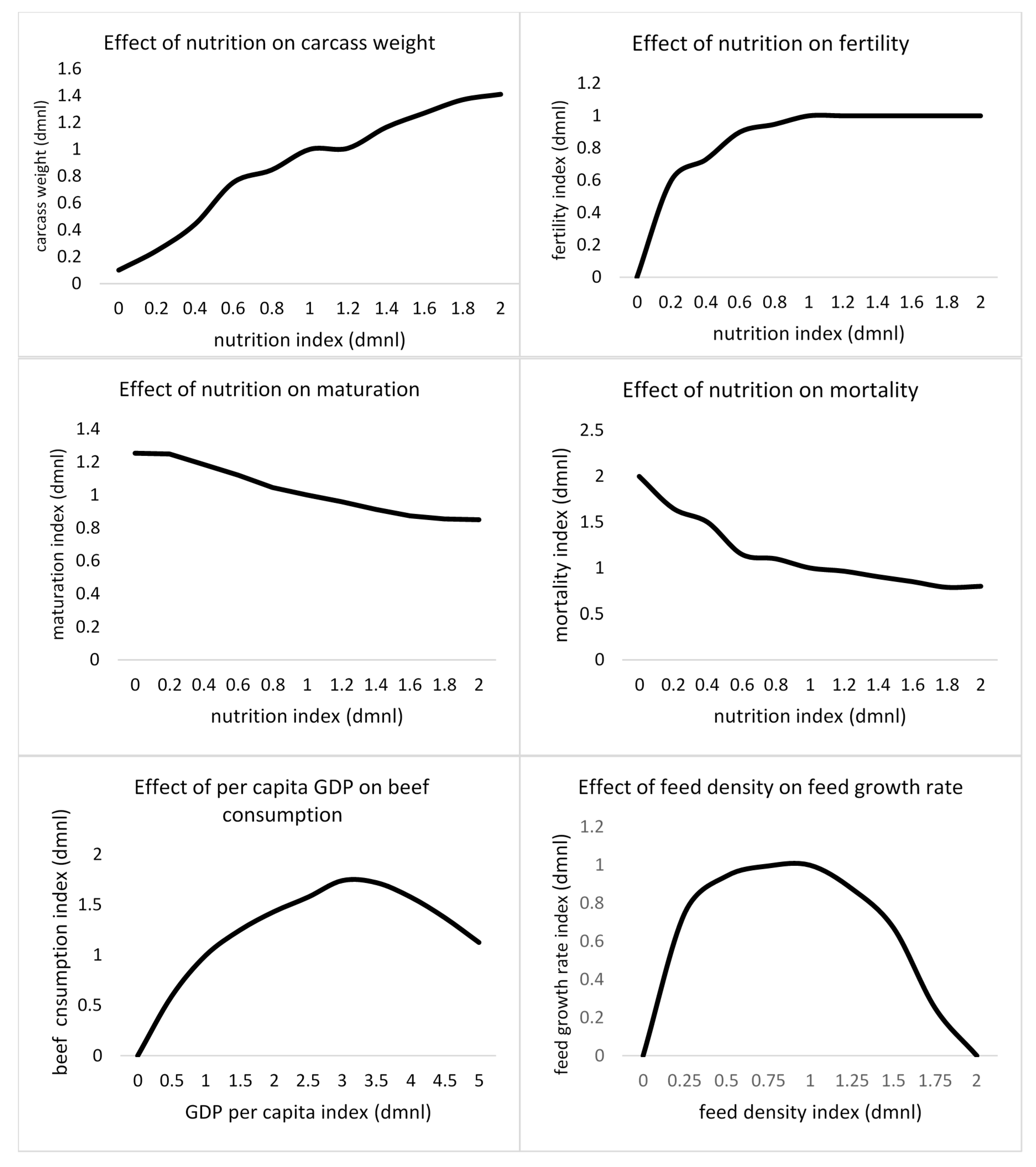
Appendix A provides all graphical functions (Figure A1) used in the model along with assumptions used for their creation. The full Stella Architect model can be accessed via this link https://drive.google.com/open?id=1CQm_00jyGE0VLjP1zUpBzQsDidVX78H1.
Figure A1.
Graphical functions used in the model.

Assumptions used to develop graphical functions:
- The indexes measure the change of the variable over time which makes the unit of each axis dimensionless. Indexes adjust values so that they are normalized relative to a chosen given starting point in time (here 1991) which is necessary to enable comparison of data. In Figure A1, an index value of 1 shows no change in trend of the variable over time, while values above or below 1 show an increasing or decreasing trend, respectively. Using indexes instead of absolute numbers is considered good modeling practice as it tends to prevent errors and makes reasoning easier (e.g., if “x doubles, how will y react” is graphically much easier if x = 1 than if it is an absolute number). For these reasons, some modeling software give a warning if dimensioned arguments are used in graphical functions.
- Effect of nutrition on carcass yield: Lower nutrition index (NI, the ratio of feed density to required feed density; the aim of the NI is to provide a statistic for which the nutritional deficit in cattle can be measured) causes lower carcass yield. As such, at the extreme where NI = 0 carcass yield will drop by 90%, and when NI < 1 carcass yield will not be influenced by nutrition.
- Effect of nutrition on fertility rate: A lower nutrition index leads to lower fertility rates while a NI of 1 and above shows a normal fertility rate. At the point where NI is zero, we assumed that the effect of nutrition on fertility rate will be zero, and then at points where NI is above 1 the fertility rate effects remain 1, even though more feed does not necessarily lead to higher fertility rate in cow.
- Effect of nutrition on maturation rate: A lower nutrition index leads to a higher maturation time. For instance, at one end point where NI is zero, we anticipated a 25% rise in maturation time; where NI = 1 we expected cattle to mature at their normal rate; and when NI > 1 cattle will take less time to mature, but not less than 85% of the normal maturation rate.
- Effect of nutrition on mortality rate: A nutrition index (NI, the ratio of feed density to required feed density) <1 leads to increased mortality in cattle. For instance, at one end point where nutrition index = 0, mortality rate is expected to rise to peak level, which is twice the mortality rate at a nutrition index = 1; and at a nutrition index ≥ 1 (above the required feed density), mortality rate reduces, but not more than 20% even at a NI peak of 2.
- Effect of per capita GDP on beef consumption per capita: a low GDP per capita causes low beef consumption per capita (BCPC), and, when the GDP per capita index gets to a threshold (3, 1.7), BCPC begins to decline as higher incomes beyond such level lead to a shift from beef to non-beef protein sources.
- The effect of feed density on feed growth rate graph follows an inverted-U shape. At one extreme, where the feed density index (ratio of feed density to maximum feed density) is zero, the effect is zero, and as the feed density index rises the effect rises until the index becomes 1 (its peak point). Beyond 1, the feed growth begins to decline as there is less space and nutrients for plants to thrive upon.
- Fixed points (1, 1) for all graphs indicate that if the nutrition index remains same, the effect functions will not be active.
- The graphical functions were drawn based on qualitative a priori expectations and calibration and not from historic data, as the availability or accessibility or the required data was lacking. For instance, after several enquiries, we were unable to locally obtain historic data showing the relationship between the influence of nutrition on maturation, mortality and fatality in cows. The same was true for the relationship between feed density and feed growth rate. However, we made use of historic data for GDP per capita and beef consumption per capita as a guide to plot the effect of per capita GDP on beef consumption graph.
Appendix B. Model Variable Description
Appendix B provides a summary (Table A1) of all the variables, and their respective equations, used in the model. Table A1 indicates the variable name, type of SD model variable (converter, stock or flow), variable value, variable equation (if applicable), units and any literature or sources used to inform variable parameterization.

Table A1.
Summary of model variables.
| Variable Name | Variable Type * | Value | Equation (Where Relevant) | Unit | Source |
|---|---|---|---|---|---|
| Beef for consumption | C | E | cattle.sales_rate * carcass_yield | Tons/year | |
| Carcass yield | C | E | carcass_yield_increase_factor * normal_yield_per_carcass * effect_of_nutrition_on_carcass_yield | Tons/head | FAO http://www.fao.org/faostat/en/#data |
| Carcass yield increase factor | C | E | 1 + RAMP(carcass_yield_slope, 2019) | Dmnl (Dimensionless) | |
| Carcass yield slope | C | 0.2 | Dmnl/year | Policy | |
| Consumption per capita | C | E | beef_for_consumption/population | Tons/(People * Years) | |
| Consumption per capita (kg) | C | E | consumption_per_capita * weight_conversion | Kilograms/(People * Years) | FAO http://www.fao.org/faostat/en/#data/FBS |
| Demanded beef sales rate | C | E | population * demanded_per_capita_consumption | Tons/year | |
| Demanded per capita consumption | C | E | initial_per_capita_consumption * effect_of_per_capita_GDP_on_per_capita_consumption | Tons/person/year | |
| Demanded sales rate (head) | C | E | demanded_beef_sales_rate/normal_yield_per_carcass | Head/years | |
| Effect of nutrition on carcass yield | C | G | Dmnl | Authors’ judgement | |
| Effect of per capita GDP on per capita consumption | C | G | Dmnl | Authors’ judgement | |
| Initial per capita consumption | C | 0.002145 | Tons/person/year | Derived from FAO Dataset http://www.fao.org/faostat/en/#data/FBS | |
| Normal yield per carcass | C | 0.1427 | Tons/head | Average value of data derived from FAO Dataset http://www.fao.org/faostat/en/#data | |
| Per capita GDP index | C | E | real_per_capita_GDP/INIT (real_per_capita_GDP) | Dmnl | |
| Population | C | G | Person | https://datacatalog.worldbank.org/dataset/population-estimates-and-projections | |
| Real per capita GDP | C | G | USD/person | https://datacatalog.worldbank.org/dataset/world-development-indicators | |
| Weight conversion | C | 1000 | Kg/tons | a priori | |
| Calves | S | E | calves(t − dt) + (reproduction_rate − maturation_rate − calves_dying) * dt | Head | |
| Cows | S | E | cows(t − dt) + (maturation_rate − slaughter_rate − cows_dying) * dt | Head | http://www.fao.org/faostat/en/#data/EK |
| S for sales | S | E | S_for_sales(t − dt) + (slaughter_rate + imports − sales_rate) * dt | Head | |
| Calves dying | F | E | calves * average_mortality_rate * effect_of_nutrition_on_mortality {UNIF} | Head/year | |
| Cows dying | F | E | cows * average_mortality_rate * effect_of_nutrition_on_mortality {UNIF} | Head/year | |
| Imports | F | G | Head/year | https://stats.oecd.org/Index.aspx?DataSetCode=HIGH_AGLINK_2018# | |
| Maturation rate | F | E | DELAYN(reproduction_rate − calves_dying, maturation_time, maturation_delay_order, reproduction_rate − calves_dying) {UNIF} | Head/year | |
| Reproduction rate | F | E | DELAYN(breeding_S * fertility_rate * effect_of_nutrition_on_fertility, gestation_period, reproduction_delay_order, breeding_S * fertility_rate * effect_of_nutrition_on_fertility) {UNIF} | Head/year | |
| Sales rate | F | E | DELAYN(slaughter_rate + imports, beef_storage_time, beef_storage_time_delay_order, slaughter_rate + imports) {UNIF} | Head/year | |
| Slaughter rate | F | E | (MIN ((cows/time_to_slaughter) − cows_dying, Beef_Market.”demanded_sales_rate_(head)”)) * IF(TIME > policy_start_time AND(TIME < policy_stop_time)) THEN (1 − slaughter_rate_reduction_fraction) ELSE 1 {UNIF} | Head/year | https://stats.oecd.org/Index.aspx?DataSetCode=HIGH_AGLINK_2018# |
| Average maturation time | C | 1.7 | Years | Various literature review | |
| Average mortality rate | C | 0.01 | Dmnl/year | Authors’ judgement | |
| Beef storage time | C | 0.1667 | Year | During calibration process | |
| Beef storage time delay order | C | 5.3 | Dmnl | During calibration process | |
| Breeding proportion | C | 0.2335 | Dmnl | During calibration process | |
| Breeding S | C | E | cows * breeding_proportion | Head | |
| Effect of nutrition on fertility | C | G | Dmnl | Authors’ judgement | |
| Effect of nutrition on maturation | C | G | Dmnl | Authors’ judgement | |
| Effect of nutrition on mortality | C | G | Dmnl | Authors’ judgement | |
| Fertility rate | C | 1 | Dmnl/year | Scholarly articles | |
| Gestation period | C | 0.789 | Year | Scholarly articles | |
| Import future | C | G | Head/year | https://stats.oecd.org/Index.aspx?DataSetCode=HIGH_AGLINK_2018# (2019–2030) | |
| Import past | C | G | Head/year | https://stats.oecd.org/Index.aspx?DataSetCode=HIGH_AGLINK_2018# (1990–2018) | |
| Initial calves | C | 1.0 × 10⁶ | Head | During calibration process | |
| Initial cows | C | 6.97 × 10⁶ | Head | http://www.fao.org/faostat/en/#data/EK (1990) | |
| Initial S for sales | C | 1.39 × 10⁷ | Head | http://www.fao.org/faostat/en/#data/EK (1990) | |
| Maturation delay order | C | 3.83 | Dmnl | During calibration process | |
| Maturation time | C | E | effect_of_nutrition_on_maturation * average_maturation_time | Year | |
| Policy start time | C | 2019 | Year | ||
| Policy stop time | C | 2022 | Year | ||
| Present time | C | 2018 | Year | ||
| Reproduction delay order | C | 1.99 | Dmnl | During calibration process | |
| Slaughter rate reduction fraction | C | 0–1 | Dmnl | Policy | |
| Time to slaughter | C | 4.65 | Year | During calibration process | |
| Feed | S | E | feed(t − dt) + (feed_growth_rate − feed_utilization_rate) * dt | Tons | |
| Pasture | S | E | pasture(t − dt) + (pasture_increase_rate − pasture_decrease_rate) * dt | Hectares | http://faostat3.fao.org/download/R/RL/F |
| Potential pasture | S | E | potential_pasture(t − dt) + (−pasture_increase_rate) * dt | Hectares | |
| Feed growth rate | F | E | pasture * feed_growth_rate_per_hectare {UNIF} | Tons/year | |
| Feed utilization rate | F | E | Cattle.cows * feed_consumed_per_cow {UNIF} | Tons/year | |
| Pasture decrease rate | F | E | pasture/pasture_decommission_time {UNIF} | Hectare/year | |
| Pasture increase rate | F | E | MIN (extra_pasture_needed/pasture_conversion_time, potential_pasture/pasture_conversion_time) {UNIF} | Hectare/year | |
| Desired liveS density | C | 8.017 | Head/hectare | During calibration process | |
| Extra pasture needed | C | E | Cattle.cows/(desired_liveS_density—liveS_density) | Hectare | |
| Feed consumed per cow | C | 5.529 | Tons/head/year | During calibration process | |
| Feed density | C | E | feed/pasture | Tons/hectare | |
| Feed growth rate per hectare | C | 0.6779 | Tons/hectare/year | During calibration process | |
| Initial feed | C | 6.7 × 10⁸ | Tons | During calibration process | |
| Initial pasture | C | 6.15 × 10⁷ | Hectares | http://faostat3.fao.org/download/R/RL/F | |
| Initial potential pasture | C | 8.0 × 10⁸ | Hectares | http://faostat3.fao.org/download/R/RL/F | |
| LiveS density | C | E | Cattle.cows/pasture | Head/hectares | http://www.fao.org/faostat/en/#data/EK |
| Nutrition index | C | E | feed_density/starvation_threshold | Dmnl | |
| Pasture conversion time | C | 0.059 | Year | During calibration process | |
| Pasture decommission time | C | 3.992 | Year | During calibration process | |
| Required feed density | C | 14.5 | Tons/hectare | http://ecocrop.fao.org/ecocrop/srv/en/home |
* C is for Converter, F is for Flow, S is for Stock, E is for Endogenous and G is for Graphical.
References
- Scrimshaw, N.S.; Béhar, M. Protein Malnutrition in Young Children. Science 1961, 133, 2039–2047. [Google Scholar] [CrossRef]
- Müller, O.; Krawinkel, M. Malnutrition and health in developing countries. Can. Med. Assoc. J. 2005, 173, 279–286. [Google Scholar] [CrossRef] [PubMed] [Green Version]
- Batool, R.; Butt, M.S.; Sultan, M.T.; Saeed, F.; Naz, R. Protein–energy malnutrition: a risk factor for various ailments. Crit. Rev. Food Sci. Nutr. 2015, 55, 242–253. [Google Scholar] [CrossRef] [PubMed]
- Semba, R.D. The Rise and Fall of Protein Malnutrition in Global Health. Ann. Nutr. Metab. 2016, 69, 79–88. [Google Scholar] [CrossRef] [PubMed] [Green Version]
- Ittner, N.R.; Bond, T.E.; Kelly, C.F. Methods of increasing beef production in hot climates. Bull. Calif. Agric. Exp. Stn. 1958, B0761, 1–90. [Google Scholar]
- Euclides Filho, K. Supply chain approach to sustainable beef production from a Brazilian perspective. Livest. Prod. Sci. 2004, 90, 53–61. [Google Scholar] [CrossRef]
- McAlpine, C.A.; Etter, A.; Fearnside, P.M.; Seabrook, L.; Laurance, W.F. Increasing world consumption of beef as a driver of regional and global change: A call for policy action based on evidence from Queensland (Australia), Colombia and Brazil. Glob. Environ. Chang. 2009, 19, 21–33. [Google Scholar] [CrossRef]
- Martha, G.B.; Alves, E.; Contini, E. Land-saving approaches and beef production growth in Brazil. Agric. Syst. 2012, 110, 173–177. [Google Scholar] [CrossRef] [Green Version]
- Recanati, F.; Allievi, F.; Scaccabarozzi, G.; Espinosa, T.; Dotelli, G.; Saini, M. Global Meat Consumption Trends and Local Deforestation in Madre de Dios: Assessing Land Use Changes and other Environmental Impacts. Procedia Eng. 2015, 118, 630–638. [Google Scholar] [CrossRef] [Green Version]
- Herrero, M.; Thornton, P.K. Livestock and global change: emerging issues for sustainable food systems. Proc. Natl. Acad. Sci. USA 2013, 110, 20878–20881. [Google Scholar] [CrossRef] [Green Version]
- Nardone, A.; Ronchi, B.; Lacetera, N.; Ranieri, M.S.; Bernabucci, U. Effects of climate changes on animal production and sustainability of livestock systems. Livest. Sci. 2010, 130, 57–69. [Google Scholar] [CrossRef]
- McMichael, A.J.; Butler, A.J. Environmentally Sustainable and Equitable Meat Consumption in a Climate Change World, Chapter 11. In Meat Crisis: Developing More Sustainable Production and Consumption; D’Silva, J., Webster, J., Eds.; Routledge: Oxfordshire, UK, 2010. [Google Scholar]
- Smith, P.; Gregory, P.J. Climate change and sustainable food production. Proc. Nutr. Soc. 2013, 72, 21–28. [Google Scholar] [CrossRef] [PubMed] [Green Version]
- Steinfeld, H.; Gerber, P. Livestock production and the global environment: Consume less or produce better? Proc. Natl. Acad. Sci. USA 2010, 107, 18237–18238. [Google Scholar] [CrossRef] [Green Version]
- FAOSTAT. Available online: http://www.fao.org/faostat/en/#data (accessed on 5 March 2020).
- Sanders, J.O.; Cartwright, T.C. A general cattle production systems model. I: Structure of the model. Agric. Syst. 1979, 4, 217–227. [Google Scholar] [CrossRef]
- Cederberg, C.; Stadig, M. System expansion and allocation in life cycle assessment of milk and beef production. Int. J. LCA 2003, 8, 350–356. [Google Scholar] [CrossRef]
- Seré, C.; van der Zijpp, A.; Persley, G.; Rege, E. Dynamics of livestock production systems, drivers of change and prospects for animal genetic resources. Anim. Genet. Resour./Resour. génétiques Anim./Recur. genéticos Anim. 2008, 42, 3–24. [Google Scholar] [CrossRef] [Green Version]
- Tedeschi, L.O.; Nicholson, C.F.; Rich, E. Using System Dynamics modelling approach to develop management tools for animal production with emphasis on small ruminants. Small Rumin. Res. 2011, 98, 102–110. [Google Scholar] [CrossRef] [Green Version]
- Sterman, J.D. Business Dynamics: Systems Thinking and Modeling for a Complex World; Irwin/McGraw-Hill: New York, NY, USA, 2000. [Google Scholar]
- FAO Human Energy Requirements. Report of a Joint FAO/WHO/UNU Expert Consultation. World Health Organ. Tech. Rep. Ser. 2004, 1, 35–50. [Google Scholar]
- Food and Agriculture Organization Corporate Statistical Database (FAOSTAT). Statistical Database; Food and Agriculture Organization of the United Nations: Rome, Italy, 2013. [Google Scholar]
- Oloyede, H. All for the love of nutrients. In The Seventy Eight Inaugural Lecture, Library and Publication Committee; University of Ilorin: Ilorin, Nigeria, 2005. [Google Scholar]
- Von Braun, J. The World Food Situation: An Overview; IFPRI Policy Brief: Washington, DC, USA, 2005. [Google Scholar]
- Ajayi, A.; Chukwu, M. Soybean Utilisation Among Households in Nslia Local Government Area of Enugu State: Implications for the’Women-in-Agriculture’Extension Programme. In Department of Agricultural Extension; University of Nigeria: Nsukka, Nigeria, 2008; p. 1118-0021. [Google Scholar]
- Adetunji, M.; Adepoju, A. Evaluation of households protein consumption pattern in offrire local government area of Oyo State. Int. J. Agric. Econ. Rural. Dev. 2011, 4, 72–82. [Google Scholar]
- Garner, T.I. Consumer expenditures and inequality: an analysis based on decomposition of the Gini coefficient. Rev. Econ. Stat. 1993, 75, 134–138. [Google Scholar] [CrossRef]
- Farrow, A.; Larrea, C.; Hyman, G.; Lema, G. Exploring the spatial variation of food poverty in Ecuador. Food Policy 2005, 30, 510–531. [Google Scholar] [CrossRef] [Green Version]
- Nasurudeen, P.; Kuruvila, A.; Sendhil, R.; Chandresekar, V. The dynamics and inequality of nutrient consumption in India. Indian J. Agric. Econ. 2006, 61, 362–373. [Google Scholar]
- Cirera, X.; Masset, E. Income distribution trends and future food demand. Philos. Trans. R. Soc. B Biol. Sci. 2010, 365, 2821–2834. [Google Scholar] [CrossRef] [PubMed]
- FAO and GDP. Climate Change and the Global Dairy Cattle Sector—The Role of the Dairy Sector in Low-Carbon Future; FAO: Rome, Italy, 2018; p. 36. [Google Scholar]
- Parsons, D.; Nicholson, C.F.; Blake, R.W.; Ketterings, Q.M.; Ramírez-Aviles, L.; Fox, D.G.; Tedeschi, L.O.; Cherney, J.H. Development and evaluation of an integrated simulation model for assessing smallholder crop–livestock production in Yucatán, Mexico. Agric. Syst. 2011, 104, 1–12. [Google Scholar] [CrossRef] [Green Version]
- Stephens, E.C.; Nicholson, C.F.; Brown, D.R.; Parsons, D.; Barrett, C.B.; Lehmann, J.; Mbugua, D.; Ngoze, S.; Pell, A.N.; Riha, S.J. Modeling the impact of natural resource-based poverty traps on food security in Kenya: The Crops, Livestock and Soils in Smallholder Economic Systems (CLASSES) model. Food Sec. 2012, 4, 423–439. [Google Scholar] [CrossRef]
- McRoberts, K.C.; Nicholson, C.F.; Blake, R.W.; Tucker, T.W.; Padilla, G.D. Group Model Building to Assess Rural Dairy Cooperative Feasibility in South-Central Mexico. Int. Food Agribus. Manag. Rev. 2013, 16, 55. [Google Scholar]
- Walters, J.P.; Archer, D.W.; Sassenrath, G.F.; Hendrickson, J.R.; Hanson, J.D.; Halloran, J.M.; Vadas, P.; Alarcon, V.J. Exploring agricultural production systems and their fundamental components with system dynamics modelling. Ecol. Model. 2016, 333, 51–65. [Google Scholar] [CrossRef] [Green Version]
- Kahn, H.E.; Lehrer, A.R. A dynamic model for the simulation of cattle herd production systems: Part 3—Reproductive performance of beef cows. Agric. Syst. 1984, 13, 143–159. [Google Scholar] [CrossRef]
- Neto, R.d.C.S.; Berchin, I.I.; Magtoto, M.; Berchin, S.; Xavier, W.G.; Guerra, J.B.S.O.d.A. An integrative approach for the water-energy-food nexus in beef cattle production: A simulation of the proposed model to Brazil. J. Clean. Prod. 2018, 204, 1108–1123. [Google Scholar] [CrossRef]
- Li, M.; Fu, Q.; Singh, V.P.; Ji, Y.; Liu, D.; Zhang, C.; Li, T. An optimal modelling approach for managing agricultural water-energy-food nexus under uncertainty. Sci. Total. Environ. 2019, 651, 1416–1434. [Google Scholar] [CrossRef]
- Pang, H.; Makarechian, M.; Basarab, J.; Berg, R. Structure of a dynamic simulation model for beef cattle production systems. Can. J. Anim. Sci. 1999, 79, 409–417. [Google Scholar] [CrossRef]
- Turner, B.L.; Menendez, H.M.; Gates, R.; Tedeschi, L.O.; Atzori, A.S. System Dynamics Modeling for Agricultural and Natural Resource Management Issues: Review of Some Past Cases and Forecasting Future Roles. Resources 2016, 5, 40. [Google Scholar] [CrossRef] [Green Version]
- Ash, A.; Hunt, L.; McDonald, C.; Scanlan, J.; Bell, L.; Cowley, R.; Watson, I.; McIvor, J.; MacLeod, N. Boosting the productivity and profitability of northern Australian beef enterprises: Exploring innovation options using simulation modelling and systems analysis. Agric. Syst. 2015, 139, 50–65. [Google Scholar] [CrossRef] [Green Version]
- Guimarães, V.P.; Tedeschi, L.O.; Rodrigues, M.T. Development of a mathematical model to study the impacts of production and management policies on the herd dynamics and profitability of dairy goats. Agric. Syst. 2009, 101, 186–196. [Google Scholar] [CrossRef]
- Gebre, K.T.; Wurzinger, M.; Gizaw, S.; Haile, A.; Rischkowsky, B.; Sölkner, J. Effect of genetic improvement of body weight on herd dynamics and profitability of Ethiopian meat sheep: A dynamic simulation model. Small Rumin. Res. 2014, 117, 15–24. [Google Scholar] [CrossRef]
- Babatunde, R.O.; Qaim, M. Impact of off-farm income on food security and nutrition in Nigeria. Food Policy 2010, 35, 303–311. [Google Scholar] [CrossRef]
- Agboola, M.O.; Balcilar, M. Impact of food security on urban poverty: a case study of Lagos State, Nigeria. Procedia-Soc. Behav. Sci. 2012, 62, 1225–1229. [Google Scholar] [CrossRef] [Green Version]
- ‘Lagos consumes N1.6bn Worth of Cattle Daily’–Punch Newspapers. Available online: https://punchng.com/lagos-consumes-n1-6bn-worth-cattle-daily/ (accessed on 5 March 2020).
- Mshelbwala, G. National Livestock Policy Focal Point Presentation–Nigeria. In Proceedings of the Side-Meeting of NLPFPS on VET-GOV Programme Engagement/Targetting and Capacity Building Facilitation. Abuja, Nigeria. Available online: http://www.au-ibar.org/component/jdownloads/finish/67-vet-gov-presentations/1427-nigeria-national-livestock-policy-focal-point-presentation (accessed on 15 February 2020).
- Olukunle, O.T. Challenges and prospects of agriculture in Nigeria: the way forward. J. Econ. Sustain. Dev. [Internet] 2013, 4, 37–45. [Google Scholar]
- Kamuanga, M.J.; Somda, J.; Sanon, Y.; Kagoné, H. Livestock and Regional Market in the Sahel and West Africa: Potentials and Challenges; Sahel and West Africa Club/OECD: Paris, France, 2008. [Google Scholar]
- Suleiman, A.; Jackson, E.L.; Rushton, J. Challenges of pastoral cattle production in a sub-humid zone of Nigeria. Trop. Anim. Health Prod. 2015, 47, 1177–1185. [Google Scholar] [CrossRef]
- Akinyemi, T.E. Climate Change Adaptation and Conflict Prevention: Innovation and Sustainable Livestock Production in Nigeria and South Africa. In Nigeria-South Africa Relations and Regional Hegemonic Competence; Springer: Berlin, Germany, 2019; pp. 87–108. [Google Scholar]
- Olabisi, H.A.; Rasheed, A.S. Evaluation of Challenges Facing Small Ruminants Production in Oyo Metropolis, Southern Guinea Savanna Environment of Nigeria. Int. J. Agric. For. Fish. 2017, 5, 34. [Google Scholar]
- OECD Data Live Dataset. Available online: https://stats.oecd.org/Index.aspx?DataSetCode=DP_LIVE (accessed on 7 March 2020).
- Spector, J.M.; Christensen, D.L.; Sioutine, A.V.; McCormack, D. Models and simulations for learning in complex domains: using causal loop diagrams for assessment and evaluation. Comput. Hum. Behav. 2001, 17, 517–545. [Google Scholar] [CrossRef]
- Richardson, G.P.; Black, L.J.; Deegan, M.; Ghaffarzadegan, N.; Greer, D.; Kim, H.; Luna-Reyes, L.F.; MacDonald, R.; Rich, E.; Stave, K.A.; et al. Reflections on peer mentoring for ongoing professional development in system dynamics. Syst. Dyn. Rev. 2015, 31, 173–181. [Google Scholar] [CrossRef] [Green Version]
- Free Data, Statistics, Analysis, Visualization & Sharing-Knoema.Com. Available online: https://knoema.com// (accessed on 7 March 2020).
- Refugees, U.N.H.C. for Refworld | Transforming Our World: The 2030 Agenda for Sustainable Development. Available online: https://www.refworld.org/docid/57b6e3e44.html (accessed on 25 March 2020).
- Homer, J.B. Partial-model testing as a validation tool for system dynamics (1983). Syst. Dyn. Rev. 2012, 28, 281–294. [Google Scholar] [CrossRef]
- Oliva, R. Model calibration as a testing strategy for system dynamics models. Eur. J. Oper. Res. 2003, 151, 552–568. [Google Scholar] [CrossRef]
- Architect, S. Isee Systems. Available online: https://www.iseesystems.com/store/products/stella-architect.aspx (accessed on 2 August 2019).
Figure 1.
(a) Beef consumption per capita trend in Nigeria, used as the model reference mode. (b) Protein supply from various animal sources. (c) Local production of beef and import values in Nigeria. Source: Organization for Economic Co-operation and Development (OECD) [53].
Figure 1.
(a) Beef consumption per capita trend in Nigeria, used as the model reference mode. (b) Protein supply from various animal sources. (c) Local production of beef and import values in Nigeria. Source: Organization for Economic Co-operation and Development (OECD) [53].


Figure 2.
Model development process.

Figure 3.
Causal loop diagram of the Nigerian beef system; key feedback loops are highlighted.

Figure 4.
Top-level model structure composing the beef system.

Figure 5.
Stock flow diagram of the Pasture–Feed module (The naming convention in the Stella SD software is modulename.variable-name, so that Cattle.cows indicates that the cows stock variable comes from the Cattle module.).
Figure 5.
Stock flow diagram of the Pasture–Feed module (The naming convention in the Stella SD software is modulename.variable-name, so that Cattle.cows indicates that the cows stock variable comes from the Cattle module.).

Figure 6.
Stock flow diagram of the Cattle module.

Figure 7.
Stock flow diagram of the Beef Market module.

Figure 8.
Graph of BCPC (in kg/capita/y) under various scenarios.

© 2020 by the authors. Licensee MDPI, Basel, Switzerland. This article is an open access article distributed under the terms and conditions of the Creative Commons Attribution (CC BY) license (http://creativecommons.org/licenses/by/4.0/).
Share and Cite
MDPI and ACS Style
Odoemena, K.G.; Walters, J.P.; Kleemann, H.M. A System Dynamics Model of Supply-Side Issues Influencing Beef Consumption in Nigeria. Sustainability 2020, 12, 3241. https://0-doi-org.brum.beds.ac.uk/10.3390/su12083241
AMA Style
Odoemena KG, Walters JP, Kleemann HM. A System Dynamics Model of Supply-Side Issues Influencing Beef Consumption in Nigeria. Sustainability. 2020; 12(8):3241. https://0-doi-org.brum.beds.ac.uk/10.3390/su12083241
Chicago/Turabian StyleOdoemena, Kelechukwu G., Jeffrey P. Walters, and Holger Maximilian Kleemann. 2020. "A System Dynamics Model of Supply-Side Issues Influencing Beef Consumption in Nigeria" Sustainability 12, no. 8: 3241. https://0-doi-org.brum.beds.ac.uk/10.3390/su12083241
Note that from the first issue of 2016, this journal uses article numbers instead of page numbers. See further details here.