
A Holistic Multi-Objective Design Optimization Approach for Arctic Offshore Supply Vessels


1
Department of Mechanical Engineering, Aalto University, FI-00076 Aalto, Finland
2
Department of Fleet Operations, Central Marine Research and Design Institute, 191015 St. Petersburg, Russia
*
Author to whom correspondence should be addressed.
Sustainability 2021, 13(10), 5550; https://0-doi-org.brum.beds.ac.uk/10.3390/su13105550
Submission received: 22 March 2021
/
Revised: 6 May 2021
/
Accepted: 13 May 2021
/
Published: 16 May 2021
(This article belongs to the Special Issue Environmental Risk Assessment of Marine Activities in Ice-Covered Waters towards Sustainability)
Abstract
:This article presents a new holistic multi-objective design approach for the optimization of Arctic Offshore Supply Vessels (OSVs) for cost- and eco-efficiency. The approach is intended to be used in the conceptual design phase of an Arctic OSV. It includes (a) a parametric design model of an Arctic OSV, (b) performance assessment models for independently operating and icebreaker-assisted Arctic OSVs, and (c) a novel adaptation of the Artificial Bee Colony (ABC) algorithm for multi-objective optimization of Arctic OSVs. To demonstrate the feasibility and viability of the proposed optimization approach, a series of case studies covering a wide range of operating scenarios are carried out. The results of the case studies indicate that the consideration of icebreaker assistance significantly extends the feasible design space of Arctic OSVs, enabling solutions with improved energy- and cost-efficiency. The results further indicate that the optimal amount of icebreaking assistance and optimal vessel speed differs for different vessels, highlighting the motivation for holistic design optimization. The applied adaptation of the ABC algorithm proved to be well suited and efficient for the multi-objective optimization problem considered.
1. Introduction
As per York and Bell [1], it took more than 50 years for oil and gas to replace oil and wood as the primary energy sources. Although there have been significant advances in science and technology since the 20th century, the ongoing transition from fossil fuel to renewable energy sources is expected to take decades to complete. To power this transition, a steady and as clean as possible supply of oil and gas is needed. In this context, the Arctic shelf, which is estimated to contain some 90 billion barrels of oil and 47 trillion cubic meters of natural gas, is expected to play a significant role [2].
A significant part of the Arctic oil and gas reserves is located under the seafloor in areas featuring thick sea ice for most of the year. The development of such locations requires a complex infrastructure, including an offshore installation, a coastal supply base, and an ice-going support fleet. Arctic Offshore Supply Vessels (OSVs) are a part of the support fleet providing year-round transportation of goods and supplies between the coastal supply base and the offshore installation.
An Arctic OSV is necessarily complex as it must serve both as a cargo ship and icebreaker. Because the acquisition and operation costs of such vessels tend to be high, cost-efficiency is important. Along the lines of Watson [3], a vessel’s cost efficiency can be measured by various metrics, including the Required Freight Rate (RFR), defined as the break-even revenue per transported cargo unit (USD/t). For sustainable operations, an Arctic OSV should not only be cost efficient but also eco-efficient. This is a challenge considering that Arctic OSVs, in comparison with equivalent non-Arctic ships, typically require significantly more propulsion power to enable safe and efficient operations both in open water and in ice. To promote the use of energy-efficient ships, the International Maritime Organization has introduced the Energy Efficiency Design Index (EEDI) regulations [4]. Specifically, the EEDI regulations regulate a ship’s allowable EEDI, indicating the maximum amount of CO2 emissions per unit of transport work (grams of CO2 per ton–nautical mile) [5]. Trivyza et al. [6] encourage the development of new models to calculate a vessel’s lifetime CO2 emissions for EEDI that consider its total lifecycle and non-linear power consumption.
As per Tarovik et al. [7], towards sustainable development of Arctic offshore resources, it is necessary to develop multi-objective optimization of OSVs, considering both internal factors (e.g., the technical characteristics of a ship and related constraints) and external factors (e.g., environmental, logistical, and market-driven factors such as the price of fuel). For the consideration of such factors, Papanikolaou et al. [8] present a holistic approach that contains (a) a parametric model of the vessel considered, (b) a model representing the vessel’s performance in the external operational context, and (c) an optimization algorithm.
Approaches for holistic vessel optimization have been applied successfully on open water ships. For instance, Gutsch et al. [9] and Marques et al. [10] present single-objective optimization approaches for offshore construction vessels and liquefied natural gas carriers. Multi-objective optimization approaches using genetic algorithms have been developed for open water containerships by Priftis et al. [11], for tankers and bulk carriers by Kanellopoulou et al. [12], for Ro-Ro vessels by Skoupas et al. [13], and for high-speed boats by Peri [14]. The approaches by Peri [14] and Martins et al. [15] represent an original adaptation of the genetic algorithm. Ray et al. [16] present applications of the Hooke and Jeeves method and the Rosenbrock method for multi-objective optimization of open water ships.
Sailing ice is associated with ice resistance and ice loads, which may significantly affect a ship’s speed and performance [17]. Therefore, spatial and temporal variations in the prevailing ice conditions are a challenge with regards to providing steady year-round transportation of cargo. The effects of sea ice can be mitigated by ship design measures (e.g., hull-ice strengthening, adaptations of the hull form, and added machinery power). However, increasing a ship’s icebreaking capabilities generally has drawbacks such as increased lightweight, reduced cargo capacity, added open water resistance, reduced seakeeping performance, and increased building and operating costs. An alternative way to mitigate the effects of sea ice is to use icebreaker assistance. However, the use of icebreaker assistance is associated with significant added costs in the form of icebreaker fees. Considering the above, when designing an Arctic OSV, it is necessary to make tradeoffs between multiple different design considerations. To the knowledge of the authors, presently there is no appropriate approach for this purpose.
Recent studies in Arctic maritime engineering provide a theoretical basis to develop a holistic optimization approach for Arctic ships. Bergström et al. [18] investigated the impact of stochastic factors and uncertainties on the design of ships and maritime transport systems for ice-infested waters. Topaj et al. [19] presented an ice routing optimization approach for a ship with icebreaker assistance. Dobrodeev and Sazonov [20] presented a method for estimating the impact of icebreaking assistance on the EEDI. Kondratenko and Tarovik [21] developed a parametric design model of an Arctic offshore support vessel.
It is noted that any new multi-objective optimization approach is an adaptation of some existing single-objective optimization algorithm [14,22]. Multi-objective optimization implies no single optimal solution but a set of Pareto-optimal solutions [8,22]. This means that in most cases, the improvement of one objective results in the deterioration of another. A Pareto front presents the optimization results in graphical form with the objectives plotted on the axis as an outcome of a Pareto optimization. When conducting a Pareto optimization, the main challenge is to obtain a well-informative Pareto front covering the whole design space.
An optimization technique that has been successfully applied to complex practical optimization problems is the so-called Artificial Bee Colony (ABC) metaheuristic, which is based on swarm intelligence, i.e., the collective behavior of a limited collection of interacting agents or individuals [23]. A study by Karaboda and Basturk [23] indicates that the ABC algorithm, when dealing with optimizing multi-variable functions, may outperform more commonly used techniques such as the genetic algorithm. Based on this finding, we think that there is motivation to assess whether the ABC algorithm would be well suited for holistic ship design optimization as an alternative to the genetic algorithm.
Based on this background, this study aims to develop a novel holistic multi-objective optimization approach for maximizing the cost- and eco-efficiency of Arctic OSVs. To this end, the approach includes (a) a parametric design model of an Arctic OSV, (b) performance assessment models for independently operating and icebreaker-assisted Arctic OSVs, and (c) a novel adaptation of the ABC algorithm for multi-objective optimization of Arctic OSVs. In addition, the study aims to analyze how such an optimization approach would affect the design of an Arctic OSV. In fulfilling these objectives, the study addresses the following research questions (RQ):
- RQ 1: Is it feasible to apply the ABC algorithm for holistic multi-objective optimization of an Arctic vessel?
- RQ 2: How does the consideration of icebreaker assistance affect the optimization of an Arctic OSV?
- RQ 3: How does the assumed speed profile of an Arctic OSV affect the outcome of the vessel optimization process?
- RQ 4: How do variations in the cargo capacity parameters (deadweight or cargo deck area), discount rate, or operation period affect the optimization results?
2. Materials and Methods
2.1. Optimization Process
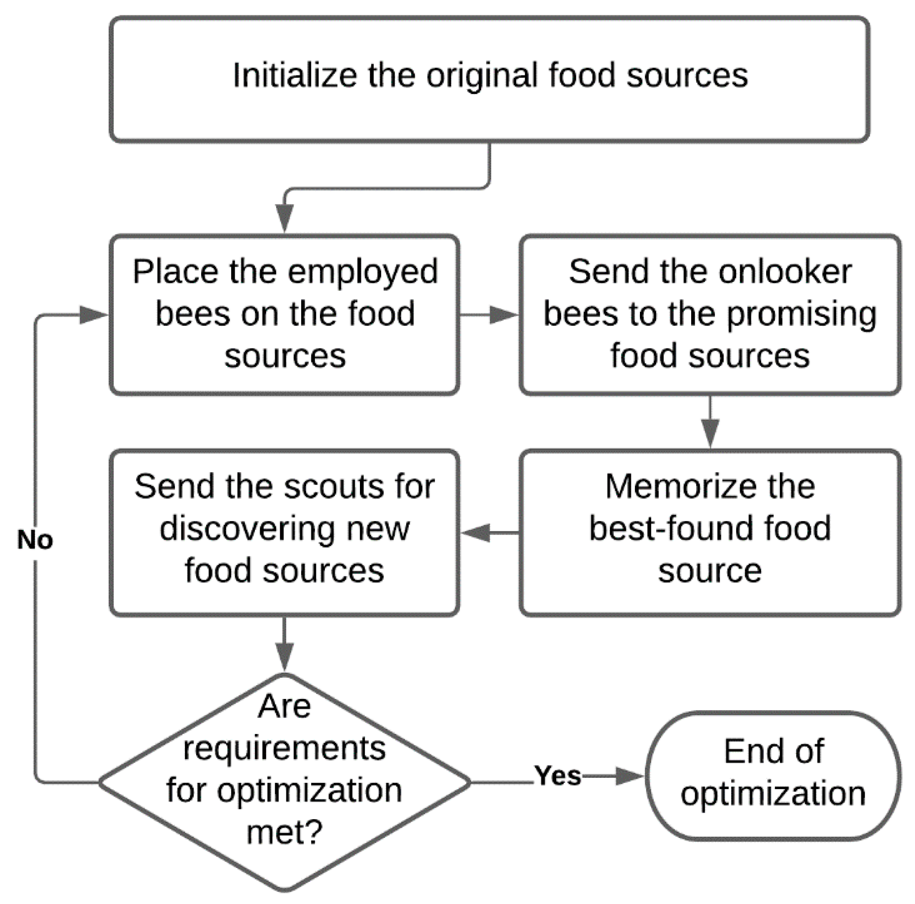
The proposed optimization approach solves a mixed-integer non-linear programming (MINLP) problem in a multi-objective formulation, applying an adaptation of the single-objective ABC algorithm. The ABC algorithm is based on the foraging strategies of honeybees [23]. A general flow chart of the ABC algorithm is presented in Figure 1. A detailed description of the algorithm is presented in [23]. Each run of the ABC algorithm results in a Pareto front point representing a single optimal solution. A vessel evaluation model supplies the ABC algorithm with an estimation of the quality of a solution in terms of cost- and eco-efficiency. The ABC algorithm operates the model as a black box, which provides information about the solution’s feasibility and evaluates the value of the objective functions considered for each set of inputs.
The objective of the algorithm is to maximize the cost- and eco-efficiency of an Arctic OSV. The cost- and eco-efficiency of a vessel is measured in terms of a cost-efficiency key performance indicator (CKPI) and an eco-efficiency key performance indicator (EKPI), determined by adapting and simplifying the definitions of RFR [3] and EEDI [5], respectively (see Section 2.2). The optimization process results in a Pareto front consisting of a set of Pareto-optimal vessel designs, representing different compromises between cost- and eco-efficiency.
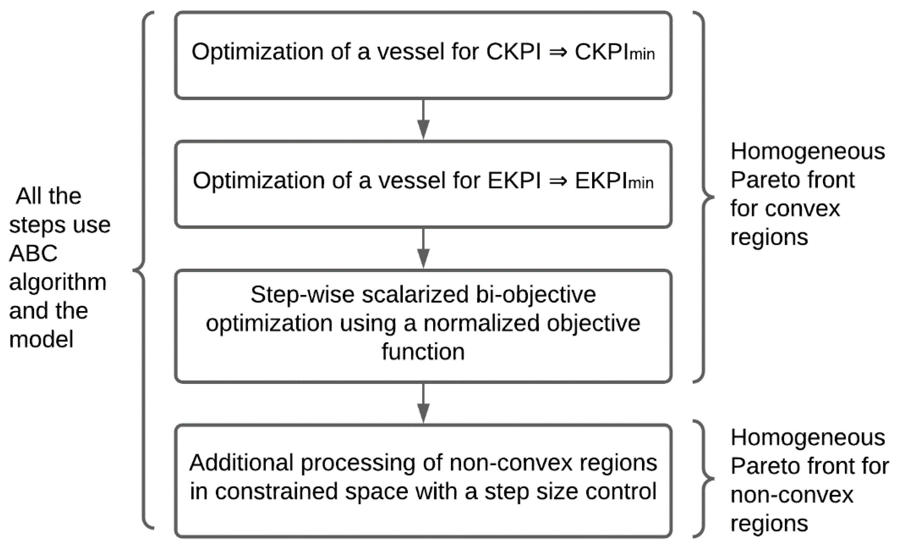
The quality of a Pareto front can be measured in terms of its homogeneity. A homogenous Pareto front is one in which the variations in the distances between consecutive points on the Pareto front are minor. This homogeneity measure is relevant because it represents the level of informativeness of a Pareto front for a decision-maker. In the case of complex scalarized optimization problems, the homogeneity often depends on the ability to find a Pareto front’s non-convex regions. This is because step-wise solution of an optimization problem using the weighted sum method can only specify the convex hull of the Pareto front [22]. In addition, the convex hull obtained will not be sufficiently homogeneous if the value ranges of the optimization objectives differ significantly from each other. This means that the concentration of the Pareto points would be unevenly distributed in favor of the objective with higher values. In Figure 2, we present a general flow chart of the algorithm to overcome these issues.
The proposed optimization process comprises two main phases. The first phase consists of a step-wise scalarized bi-objective optimization using a normalized objective function as per Equation (1). This ensures homogeneity for the convex parts of the Pareto front. The values of CKPImin and EKPImin are obtained in advance by two separate optimization runs. In the first run, CKPI is used as an optimization objective, whereas in the second run EKPI is used as an objective. This provides two boundary points of the Pareto front.
where w is a weighting factor defined in a range from 0 to 1. Starting from w = 0, the algorithm increases the value of w step-by-step by adding ∆w and finds an optimal solution, i.e., a new Pareto front point, while w < 1.
The second phase involves processing non-convex regions to provide missing points and homogeneity for the whole Pareto front. If the distance between two points exceeds a specific limit value (average distance + specific percentage × average distance), an additional constraint for either of the objectives is introduced to consider only the range between the points. Specifically, the algorithm divides the range by half and optimizes the unconstrained objective for each half of the range, resulting in two new Pareto front points. This process is repeated until the distance between all the points within the initial range is acceptable. Points that are too close to each other are dismissed.
2.2. Vessel Evaluation Model
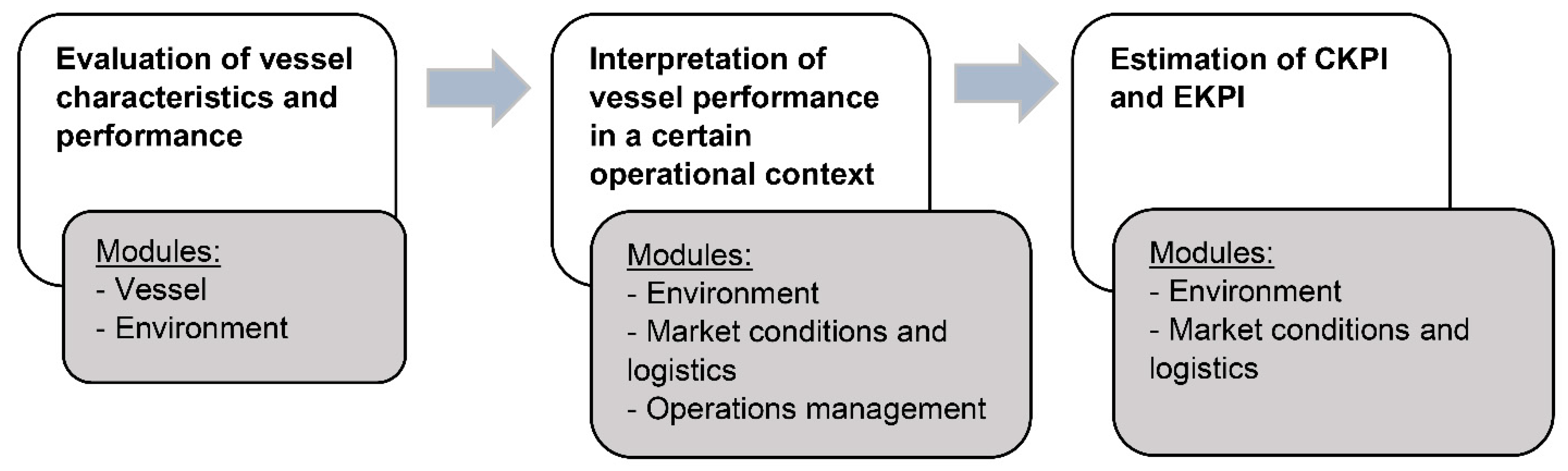
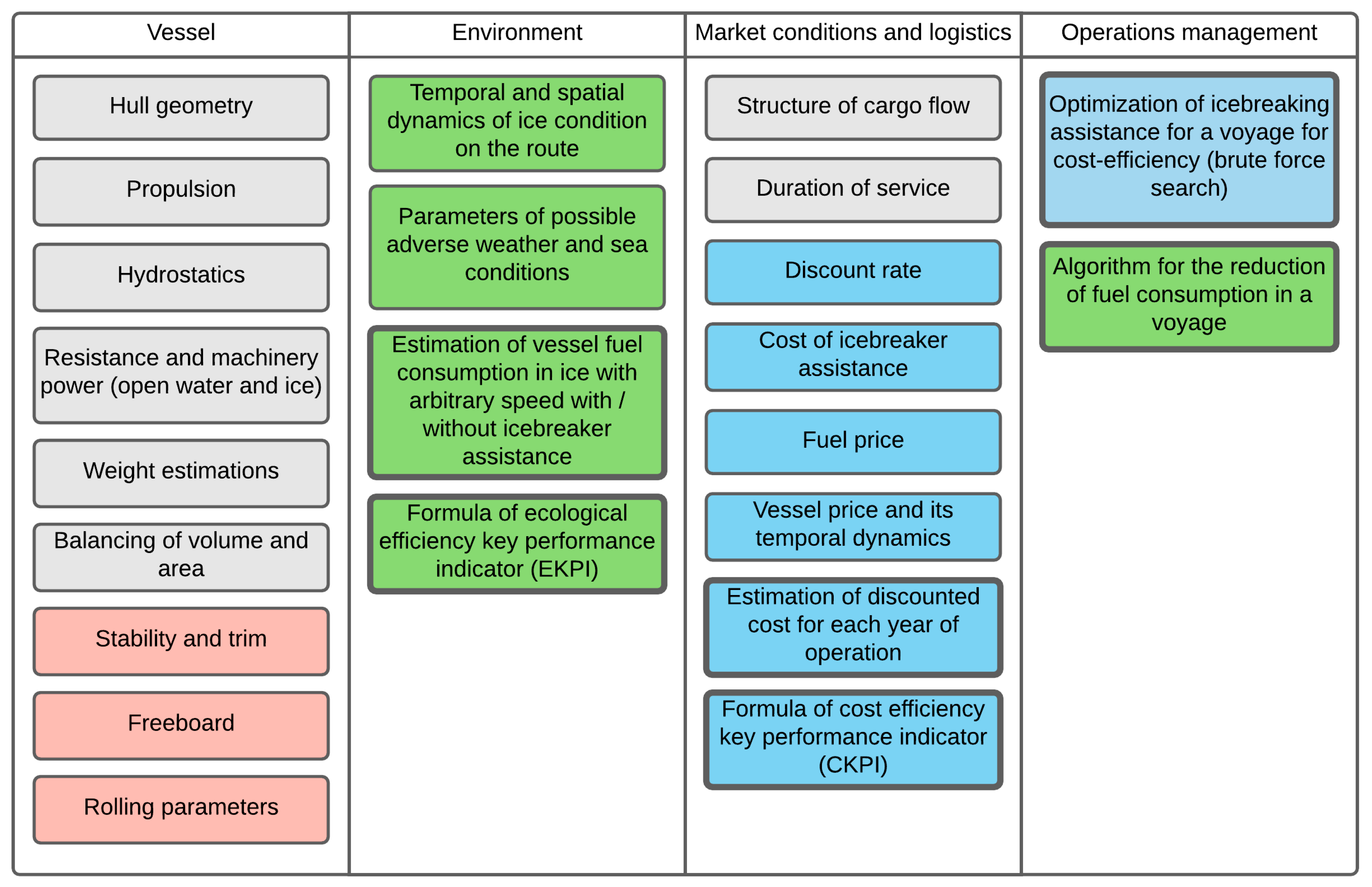
The vessel evaluation model, presented in Figure 3, estimates a vessel’s EKPI and CKPI for a given set of inputs. Figure 4 provides a module decomposition of the model. First, the model calculates a vessel’s performance, considering ship design characteristics only. Second, the model calculates a vessel’s performance in a specific operational context. We define the operational context in terms of parameters presented in Figure 4.
The vessel module (see Figure 4) is based on a holistic parametric design model of an Arctic offshore support vessel, a detailed presentation of which is provided in Kondratenko et al. [24] and Kondratenko et al. [21]. The input parameters of the model are length between perpendiculars (Lpp), beam (B), draft (T), block coefficient (Cbwl), depth (H), cruising speed in open water (Vs), ice class (Arc), and icebreaking capability (hice). The ice classes considered are determined as per the Russian Maritime Register of Shipping [25]. The vessel module considers all of the essential ship qualities and related constraints, including the hull geometry, hydrostatics and stability, resistance and propulsion (in open water and ice), required power plant capacity, general arrangement criteria, estimations of lightweight and deadweight, cargo capacity, and freeboard criteria. This study also considers an additional constraint for the maximum tolerated vessel rolling to avoid dangerous situations in adverse weather and sea conditions [26]. The rolling constraint considers related environmental characteristics of the intended operating area.
The parametric model of the vessel is verified using real-life data on Arctic and non-Arctic OSVs, including vessels with installed machinery power of up to 22,500 kW [21]. It is noted that estimations of the required hull volume for vessels with an installed machinery power exceeding 22,500 kW are questionable as the layouts of very powerful vessels (e.g., specialized icebreakers) may differ from that of conventional OSVs.
Following the specification of a vessel’s design characteristics, we calculate the necessary parameters to estimate the values of the objective functions considering the vessel’s operational context. CKPI and EKPI are determined as per Formulas (2) and (3), which we adapted to fit Arctic OSVs. In the present model, Arctic OSVs are assumed to operate year-round with the option to call for icebreaker assistance if necessary. We assume that a vessel is bought at the beginning of the project. Equation (2) determines CKPI considering revenue corresponding to the assumed resale value of the considered vessel at the end of a project. The consideration of the resale value is important as an Arctic OSV is usually bought for a specific offshore project at a significant price, meaning that a vessel’s resale revenue at the end of a project may significantly affect its overall cost efficiency. We assume that unconsidered size-dependent cost categories such as insurance, maintenance, and port fees do not significantly affect the optimization results because of OSV’s size constraints (see Section 3.1.2).
where PW (present worth) is the value of future money flows discounted to the present, calculated as ; n is the operation period (years); r is the discount rate; Nv is the number of voyages per year; and Ccap is the cargo capacity parameter (tons). The operating costs are defined as the sum of the fuel and icebreaker assistance costs. The price of icebreaker assistance per nautical mile is calculated according to [27] considering an inflation adjustment. We assume that an icebreaker assists one ship at a time for the whole voyage, meaning that there is a maximum of one instance of icebreaker assistance per voyage. The formation of convoys is not relevant due to the peculiarities of offshore logistics; operating in a convoy suggests a high concentration of vessels at one location, which would be sub-optimal considering logistical efficiency. As a simplification, the model assumes that an icebreaker is always available. This assumption is reasonable as icebreaker operators along the Northern Sea Route tend to prioritize major Arctic offshore projects. We determine the acquisition price of a ship as a function of its lightweight as per [21]. The model calculates a ship’s market value at the end of a project, assuming an annual value loss of 2% due to aging.
The model considers two different cargo capacity parameters Ccap to account for the different possible combinations of different cargo types. If the cargo to be transported is dominated by deck cargo, then Ccap = Sd·mdc, where Sd (m2) is the cargo deck area and mdc is the average density of the deck cargo (tons/ m2). An Arctic offshore installation uses fuel oil for heating, which is typically delivered by a tanker. Alternatively, supply vessels deliver the fuel. In this case, the dominating type of cargo consists of cargo carried within the hull, meaning that the vessel’s cargo carrying capacity is limited by its deadweight (Dw) so that Ccap = Dw.
Because the EEDI regulations concern neither vessels with diesel-electric propulsion nor offshore supply vessels [5], we do not specify the maximum allowed EEDI index in the present study. Instead, the model uses the EKPI index as an optimization objective for eco-efficiency as per Equation (3). It is noted, this definition of EKPI is a simplification of the original EEDI formula by the IMO [5] (e.g., it does not consider ship size-specific coefficients). In addition, contrary to the original EEDI formula that calculates a ship’s fuel consumption as a linear function of the total installed power, the applied model calculates a ship’s fuel consumption based on an approach considering its total lifecycle. This approach, which is described below, makes it possible to define EKPI and CKPI across different vessel sizes.
where CF is a conversion factor between fuel consumption and CO2 emission, and Ccap* is the cargo capacity parameter for EKPI (tons); Ccap* = Sd·mdc if the cargo is dominated by deck cargoes and Ccap* = fi·Dw if the cargo is dominated by cargos carried within the hull, where fi is the capacity correction factor for ice-classed ships [5].
We model the ice-going performance of an OSV using a dimensionless quadratic polynomial approximation of an h–v curve based on data provided in [28]. The h–v curve represents a vessel’s speed in level ice as a function of ice thickness at constant engine load. The prevailing ice conditions are modeled in terms of an equivalent ice thickness (heq), determined as per Equation (4) as a function of ice concentration (c), level ice thickness (hi), ice ridging (b), and snow cover thickness (hsn) [29]. The amount of ice ridging is quantified by integer values from 0 to 5, representing the share of ridged ice in a specific area, so that 0 indicates no ice ridging and 5 indicates 100% ridged ice.
where ksn is 0.5 if hsn ≥ 0.5 m and 0.33 otherwise.
A vessel’s h–v curve is typically specified for its maximum continuous rating (MCR) so that it indicates a vessels’ maximum attainable speed in different ice thicknesses. The assumption of operating at MCR in any ice condition is reasonable for low ice class vessels for which the power consumption at cruising speed in open water is close to the maximum continuous rating. High ice-class vessels such as Arctic OSVs, on the other hand, typically have a significant power reserve for icebreaking, resulting in a total installed machinery power that is significantly higher than what is needed to obtain a reasonable speed in open water. Therefore, for such vessels, it is not reasonable to assume continuous operations following an h–v curve calculated for the MCR.
The applied dimensionless approximation (see Equation (5)) makes it possible to draw h–v curves based on three parameters specified for a particular power output (j): attained speed in open water Vmax,j, icebreaking capability hice,j, and the speed at hice,j (V0,j, usually 2–3 knots). The methods from the vessel module [21,24] estimate the required power at various speeds. They also estimate the maximum icebreaking capability for a specific engine output. As a result, an h–v curve can be specified for any engine output.
where . is a vessel’s speed in ice with an equivalent ice thickness of using power output (j).
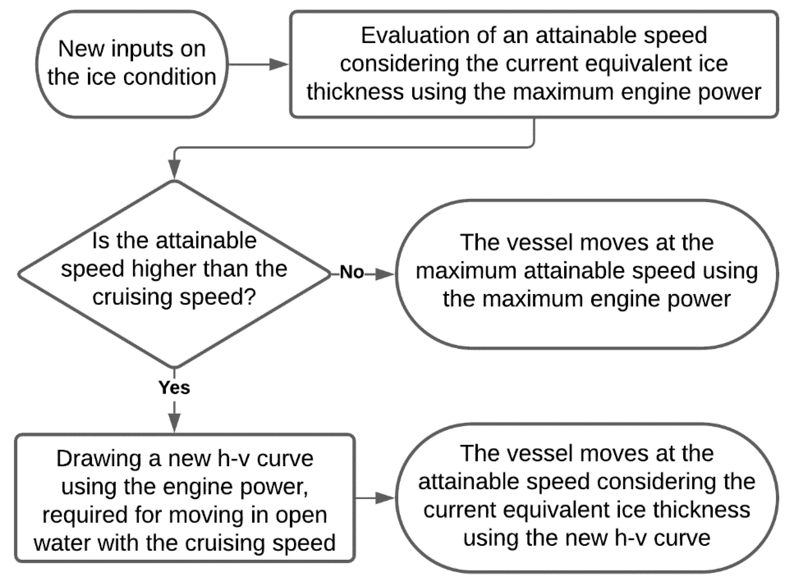
As per Figure 5, the algorithm evaluates the maximum attainable speed during independent operation considering the prevailing equivalent ice thickness. If the attainable speed is lower than the set open water cruising speed, the vessel moves at the maximum attainable speed at MCR. Otherwise, the algorithm draws a new h–v curve for a lower engine load equal to the required power for operating at the set cruising speed in open water. Thereafter, the vessel sails at the attainable speed corresponding to the updated h–v curve considering the prevailing equivalent ice thickness. Controlled by the algorithm described above, the vessel operates at MCR only in heavy ice conditions. This prevents the vessel from operating at excessively high speed in ice and open water.
An OSV often operates at low power, for example, during standby or dynamic positioning near an offshore installation. For such operations, modern diesel-electric OSVs have auxiliary diesel generators and power distribution systems providing good fuel efficiency also at low engine load. Rao et al. [30] demonstrated that OSVs equipped with power distribution systems can operate at constant specific fuel consumption (g/kWh) for machinery loads above 2000 kW. Therefore, because all vessels considered in the present study have a minimum engine load above 2000 kW, we assume that all the vessels considered have a specific fuel consumption of 221 g/kW·h regardless of machinery loads.
The algorithm is assumed to provide realistic fuel consumption estimations, providing a fair comparison of vessels with different icebreaking capabilities. For a fair comparison, the vessels’ cruising speed in open water is also included among the optimization parameters. To extend the range of feasible solutions to include vessels with moderate icebreaking capabilities, it is assumed that Arctic OSVs may obtain icebreaker assistance when facing extreme ice conditions. Icebreakers are here modeled as resources that help OSVs to increase their speed without increasing their power output. Icebreaker’s h–v curves are defined for their MCR using the dimensionless approximation described above. The speed of an icebreaker-assisted vessel is estimated according to [31] as a function of the icebreaker’s attainable speed, the prevailing navigational season (summer–autumn/winter–spring), and the ice class of the assisted vessel. This methodology is based on the real-life experience of icebreaking operations along the Northern Sea Route.
The optimization of icebreaking assistance is essential because the optimal level of assistance differ for different vessels depending on their icebreaking capabilities. We optimize the use of icebreaker assistance for cost-efficiency separately considering real-life practice. Because the assisting icebreakers are assumed to be nuclear-powered, the eco-efficiency calculations do not consider their emissions. Separately for each voyage, the algorithm decides whether a ship calls for icebreaker assistance based on an assessment of the total operating costs, calculated as the sum of fuel and icebreaker assistance costs. It is noted that due to limited icebreaking resources, it is not reasonable to assume year-round operation with icebreaking assistance provided for all vessels.
The main outcome of the model is an estimate of a vessel’s total annual fuel consumption (see Equation (6)).
where m is the month number; Nm is the average number of voyages in month m; s is the route segment number; smax is the number of segments along the route; i is the ice condition type number corresponding to the equivalent ice thickness range; imax is the number of different types of ice condition occurring along the segment s; Fm,s,i is the fuel consumption in month m for segment s in ice condition i; pm,s,i is the probability of occurrence of ice conditions of type i along the route segment s in month m; and FCO—the fuel consumption for cargo operations. The values of Nm and Fm,s,i are evaluated considering the output of the algorithms for reduced fuel consumption and optimized icebreaking assistance. The total duration of offshore cargo operations is estimated as per [21]. For port and platform cargo handling operations, the fuel consumption is assumed to be two and ten tons per day, respectively. The fuel consumption per hour is calculated by dividing the annual fuel consumption by the total annual operating hours.
3. Results
3.1. Case Study Inputs
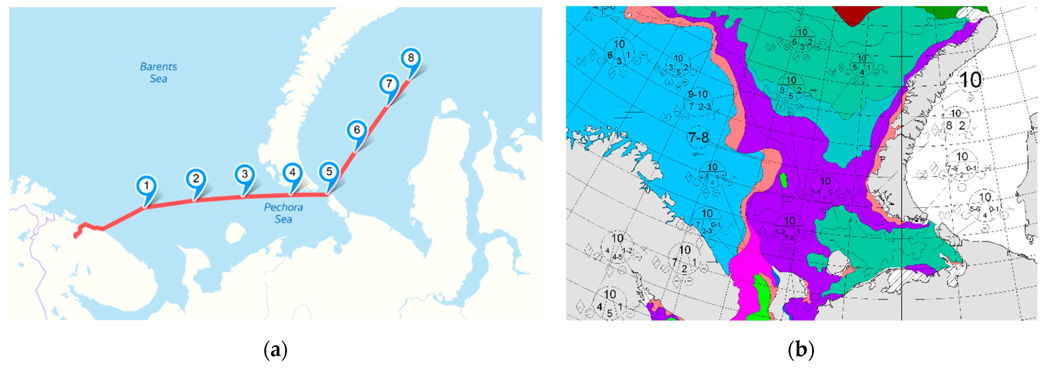
To test and demonstrate the merits of the approach, we carry out a series of case studies dealing with the optimization of an Arctic OSV for year-round operation in the northern part of the Kara Sea. Specifically, the considered offshore location to be supplied is the Pobeda field discovered by Rosneft and ExxonMobil in 2014, and the supply base considered is the port of Murmansk. The corresponding supply route is presented in Figure 6a.
3.1.1. Ice Condition
To facilitate the modeling of the ice conditions along the route, we divided the route into eight segments considering the spatial heterogeneity of the ice data. The distance between the waypoints is 100 nautical miles (n.m.) except for the open water segment between the supply base and waypoint 1 (170 n.m.), the segment between waypoints 4 and 5 (the end of the Barents Sea area, 70 n.m.), and the segment between waypoints 7 and 8 (the final segment, 70 n.m.). The ice conditions are modeled in terms of equivalent ice thickness. Ice thickness and concentration data are determined based on historical ice charts provided by AARI [32], an example of which is presented in Figure 6b. The snow cover thickness is modeled based on [33], whereas ice ridging characteristics are modeled based on [34]. The ice data cover the Barents Sea and the Kara Sea over the period 1998–2020 with a temporal resolution of one month. The ice data from the period are assumed to reflect the recent warming of the Arctic climate.
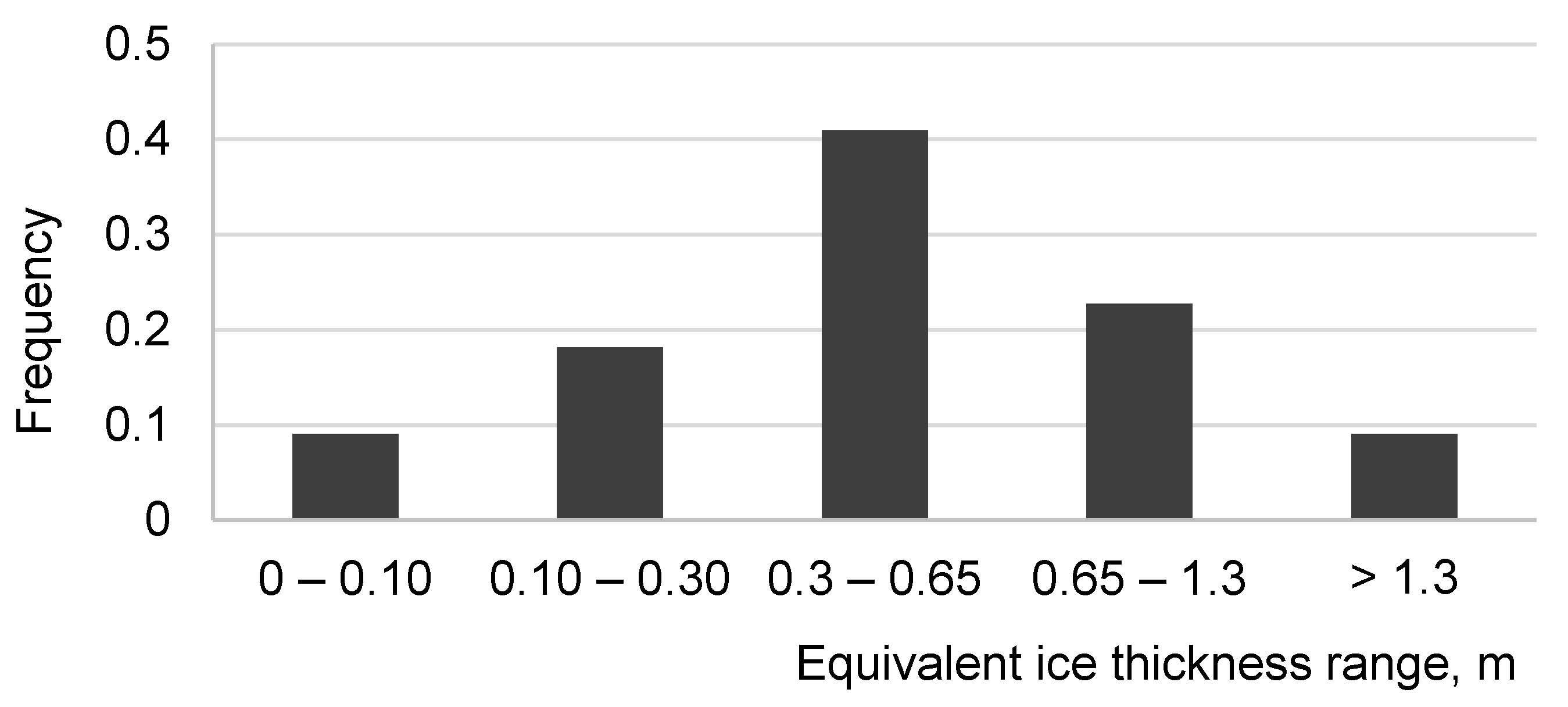
We determined the prevailing ice condition for each segment, assuming that vessels can make minor deviations from the planned route to avoid the most difficult local ice conditions. This assumption is implemented when extracting ice data from the ice charts. Based on the ice data considered, we determined ice thickness frequency distributions for each month and route segment. An example this distribution, representing segment 4–5 in March, is presented in Figure 7. As a simplification, we calculate a vessel’s performance based on the average ice thickness of a thickness range. The results were assembled into a database, which was used as input for the simulations.
3.1.2. Description of the Study Cases
Table 1 presents the parameters of seven different case studies carried out using the proposed multi-objective optimization approach. The outcomes of the case studies indicate the effects of variations in the cargo capacity parameter (Dw vs. Scargo), discount rate, operation period, and icebreaker assistance availability. A discount rate of 6% corresponds to a low-risk offshore project, whereas a discount rate of 12% corresponds to a high-risk project. We consider a fuel price of USD 400 and a 2% annual loss of the value of the considered vessel. The assisting icebreakers are assumed to be modern nuclear-powered icebreakers (hice = 2.8 m, maximum open water speed = 20.6 knots), similar to those currently operating along the Northern Sea Route. A ship’s icebreaking capability (hice) indicates the maximum equivalent ice thickness in which the ship can maintain a speed of 2 knots (V0,j = 2 knots).
Table 2 presents the range of vessel design parameter values used for all case studies. The values are determined considering a database [35] on existing open water and Arctic OSVs built within the period 1997–2017. The maximum vessel length (Lpp) considered is limited as per [7], according to which the performance and safety of an Arctic OSV suffer significantly if its Lpp exceeds the typical linear dimensions of an offshore installation (around 100 m). The maximum draft of 9 m is determined considering the minimum water depth in the operation region.
For some case studies, alternative estimates for EKPI and CKPI are calculated by deactivating the propulsion power control algorithm to demonstrate its effect on the absolute efficiency (EKPI and CKPI) and relative efficiency (compared with other solutions).
3.2. Case Study Outcomes
Figure 8 presents the optimization results for case study 1–2, which have the same discount rate (6%) but different operation periods (10 vs. 20 years). In this and all other cases, the Pareto front is smooth, generally non-convex, and close to equidistant (for the convex and non-convex regions of the Pareto front). For both charts, the EKPI values are in the same range. In the second case study, the CKPI values of the Pareto optimal vessels are considerably lower, as the increase in the amount of transported cargo outweighs the additional costs for the extended operation period. In addition, for a longer operating period (10 vs. 20 years) the effect of discounting is more significant.
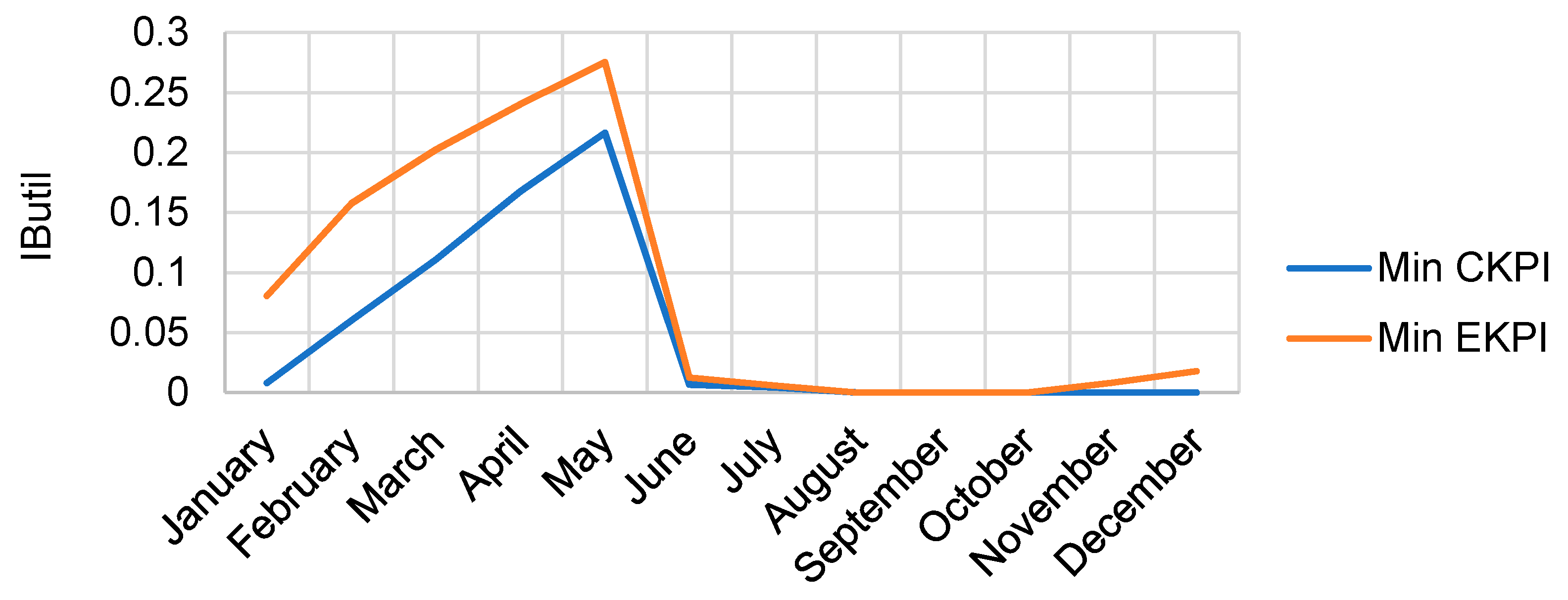
Characteristics of the vessel designs on the Pareto fronts calculated for case study 1–2, optimized for CKPI, EKPI, and an intermediate solution, are presented in Table 3, where IButil is the ratio of the total distance covered with icebreaker assistance to the total covered distance. Waterline length (Lwl) is determined as a function of Lpp and a hull form. For each case study, a list of all Pareto optimized designs is presented in Appendix A. All vessels in Table 3 determined for case study 1 have similar values of Lwl, Cbwl, and ice class, while other characteristics are different. Increasing the weight of EKPI in the objective function results in solutions with lower fuel consumption per unit of transported cargo. The corresponding designs are significantly larger, measured in terms of B, T, H, Dw, and displacement (∆). An increase in vessel size also results in higher acquisition costs, something that the EKPI index does not account for. The designs also have lower cruising speeds, which, following the applied power control algorithm, also result in reduced emissions for most ice conditions. In addition to the data provided in Table 3, Figure 9 illustrates how the value of IButil, specified per month, is changing along the year for two specific optimized vessel designs (case study 1, Min CKPI and Min EKPI). Accordingly, for both vessels, the maximum utilization of icebreaker assistance is between February to May. The vessel optimized for CKPI has a higher ice-going capability (hice), which results in lower costs for icebreaker assistance. The vessel with a higher eco-efficiency has a more frequent need for icebreaker assistance to save fuel and limit its required power plant’s capacity (Npp), resulting in a lower lightweight and increased Dw.
The characteristics of the vessel designs optimized for minimum CKPI and EKPI presented in Table 3 are similar for case study 1 and 2. The EKPI optimized vessels must be similar because those parameters that were varied in case study 1–4 impact only the value of CKPI. The latter verifies the reliability of the optimization process as the algorithm demonstrates a stable solution despite its stochastic nature.
Even though the boundary solutions (Min CKPI, Min EKPI) are similar, the intermediary solutions (Table A1 in Appendix A) were affected by variations in the length of the operation period. Specifically, an increase in operation length (case study 2) results in a considerable shift to smaller, cheaper, faster, and less environmentally friendly vessels (the average rise of EKPI is about 6.4%). The average value of displacement and Dw decreased by 7.4% and 7.5% correspondingly, caused by reduced values of B, T, and H (a drop of 4.6%, 2.5%, 2.7% correspondingly). The second cost-reducing factor, besides the acquisition cost, relates to a reduced need for icebreaker assistance, as the average utilization of IB assistance (IButil) is 12.9% lower in case study 2 than in case study 1. The average value of the vessel open water speed is also reduced by 2.1%.
The main reason for this shift is that an Arctic OSV’s resale value at the end of an offshore project is decisive for its overall cost efficiency considering its high acquisition cost. A doubled operation period results in a 20% lower vessel resale value due to aging and discounting, which forces the algorithm to find more CKPI-oriented solutions.
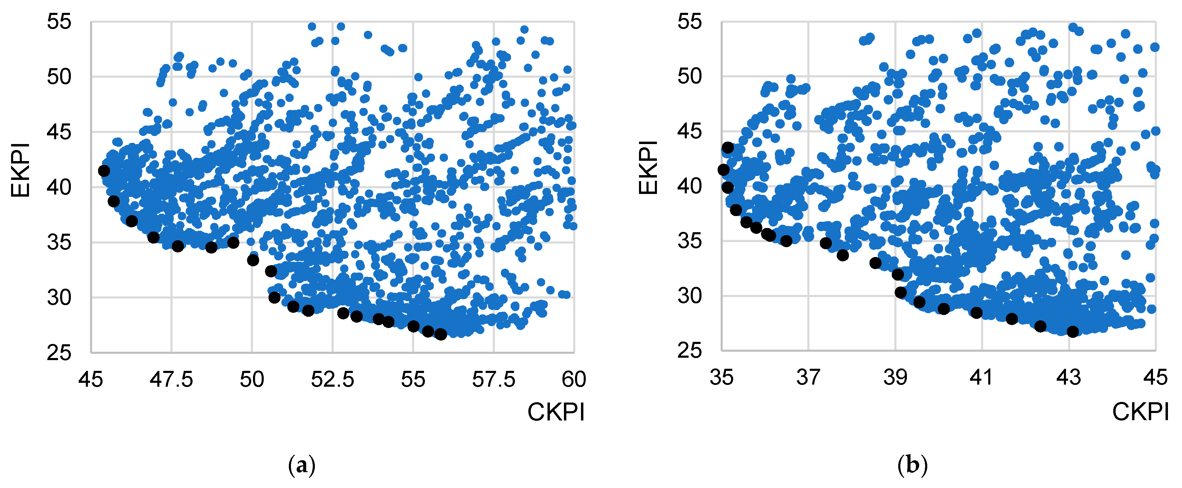
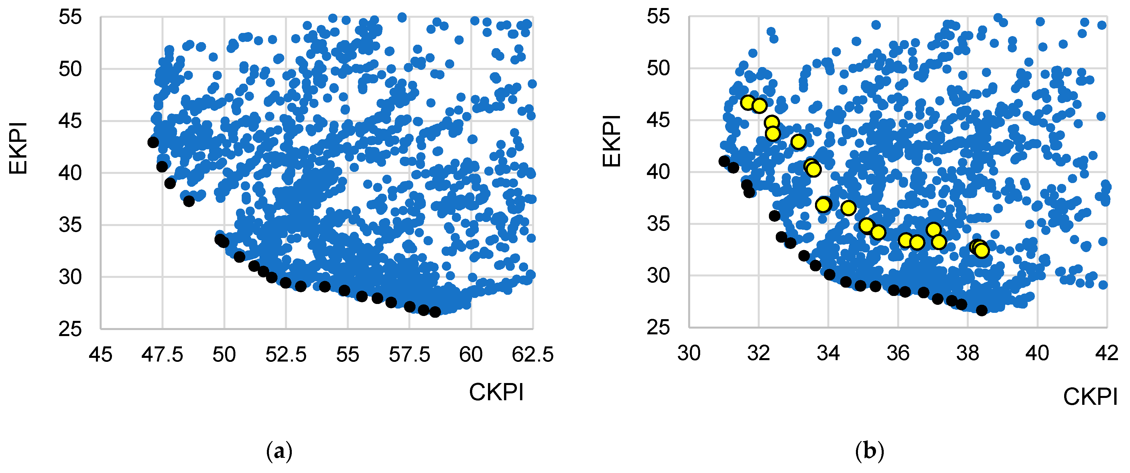
Figure 10 illustrates the Pareto fronts for case study 3 and 4 (the operation periods are 10 and 20 years respectively), which differ from the first pair of cases in terms of discount rate (12%). We provided three vessels’ characteristics, optimized for CKPI, EKPI, and an intermediate solution in Table 4. Increasing the discount rate value from 6% to 12% for a 10-year operating period (moving from case study 1 to case study 3) reduces the operation cost, while the acquisition cost remains high. The vessel purchase occurs before the commissioning, while the discounting effect becomes more significant over time. In this case, the strategy of the algorithm is to minimize a vessel’s size without increasing its negative environmental impact due to higher utilization of icebreaker assistance. This results in a decrease in the values of B, T, H, displacement and hice (2.5%, 4%, 4.2%, 6.1%, 2.3% correspondingly) and an increase in the values of Vs (2.6%) and IButil (5.2%). An additional change in the length of the period of operation from 10 to 20 years for a constant discount rate (shifting from case study 3 to case study 4) results in an insignificant variation of the vessels’ characteristics (<1%).
A demonstration of the importance of the power control algorithm applied is provided for case study 4, representing a high-risk offshore project with duration of 20 years with icebreaker availability. To consider a situation where all vessels operate at the maximum attained speed regardless of the ice conditions (the power control algorithm was deactivated), we calculated the corresponding EKPI and CKPI values for the whole range of Pareto optimal vessel designs (black points in Figure 10b). The results are presented in Figure 10b) as yellow points. As per the figure, the yellow points are shifted upwards compared to the original Pareto front, which indicates a substantial efficiency reduction, and importantly the shift is not equidistant. This means that optimizing an Arctic OSV assuming that vessels are sailing at the maximum attainable speed in ice is not sensible as the optimal speed is significantly different for different vessels. Some vessels are less efficient than others while operating at maximum speed, meaning that they would be modeled unfairly without the power control algorithm.
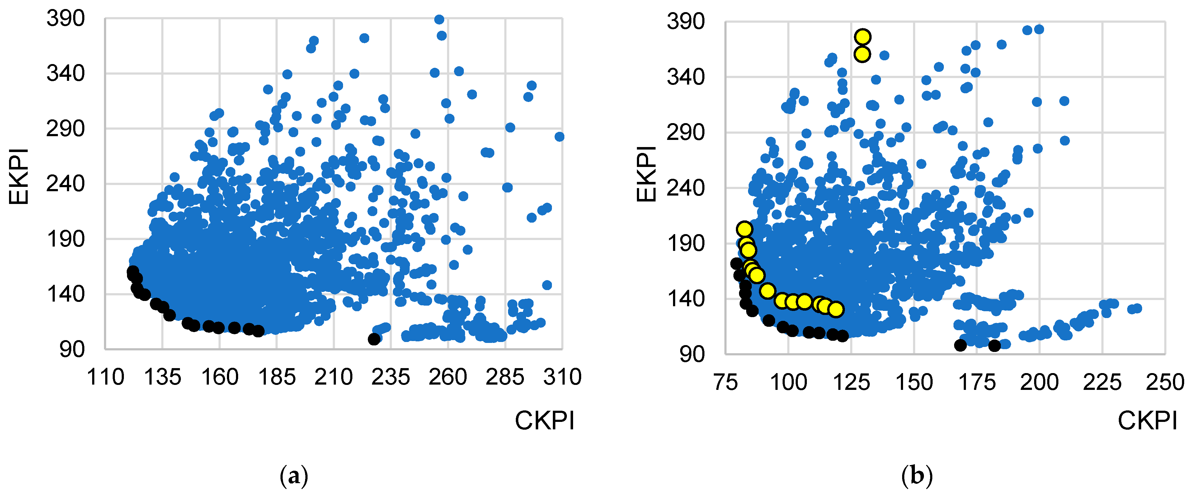
Case 5–7 suggest a change in the cargo flow pattern, as a consequence of which the required cargo capacity is defined by Scargo instead of Dw. Figure 11 presents the Pareto fronts for Case 5–6. Characteristics of vessels optimized for CKPI, EKPI, and an intermediate solution are provided in Table 5. As the results indicate, the cargo capacity parameter has the most significant impact on the optimized characteristics of an Arctic OSV. The optimal vessels in Case 5–7 are significantly smaller in size than in Case 1–4, with a significantly smaller draft and hull main particulars. The cargo deck area Scargo is associated mainly with Lwl and B when the other particulars of a hull could be minimized if design constraints are satisfied. The optimal vessels in Case 5–7 have lower Dw and internal cargo capacity values than in Case 1–4. A visualization of the optimal hull developed by the model for the intermediate solutions of Case 4 (the cargo capacity parameter is Dw) and 6 (the cargo capacity parameter is Scargo) is presented in Figure 12.
Among the optimal solutions for Case 5–6, most vessels have ice class Arc 5. The exceptions are non-typical vessels optimized for Min EKPI, which were excluded as their Npp values were almost twice the maximum set considering potential general arrangement issues. These vessels have ice class Arc 8, a high icebreaking capability (hice) of almost 2.5 m, and operate at low power when Vs is near 6.5 knots. A constrained maximum speed saves fuel both in ice and open water. The latter is important considering the significant open-water resistance of ships optimized for icebreaking. A high ice class and icebreaking capability provide lower power consumption for independent operation and operation with icebreaker assistance. Although this strategy provides the best EKPI values, CKPI values for the Arc 8 vessels are very high. Thus, as per Figure 11, for case study 5–6, those designs form a small separate group standing far on the right from the Arc 5 vessels.
The yellow points in Figure 11b represent EKPI and CKPI (Case 6) values calculated for all the Pareto optimal solutions (black points in Figure 11b) without using the power control algorithm. The conclusions are the same as for Case 4: the efficiency of the obtained vessels is significantly reduced, but the reduction varies between different vessel designs. This is especially true for vessels of ice class Arc 8, which have a very high machinery power to provide the required icebreaking capability, resulting in high fuel consumption if the vessels operate at maximum speed.
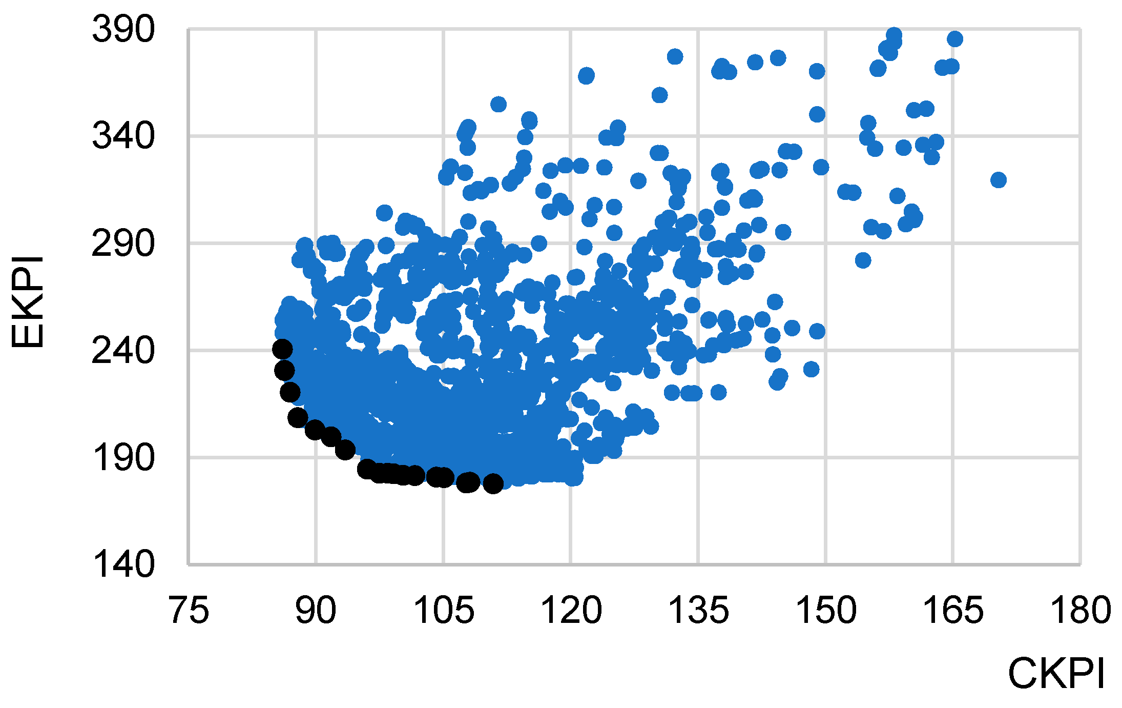
Case 7 is similar to Case 6 except that no icebreaking assistance is provided. The results of the optimization for Case 7 are presented in Figure 13. The characteristics of several optimal vessels (Min CKPI, Min EKPI, Intermediate) are presented in Table 6. In the absence of icebreaking assistance, the optimal vessels have ice class Arc 7 or Arc 8, as vessels of lower ice classes do not guarantee safe year-round, independent operation in the assumed ice conditions. Compared with Case 6, the Pareto front determined for Case 7 is shifted into a less efficient zone, which highlights the importance of icebreaking assistance. Simultaneously, the results for Case 1–7 show that the optimal amount of icebreaking assistance is different for different vessels. The latter demonstrates the importance of icebreaking assistance optimization to ensure a fair treatment of all feasible vessel designs.
4. Discussion
This article presents a framework for holistic multi-objective optimization of Arctic OSVs for cost- and eco-efficiency. The framework is intended to be used in the conceptual design phase of a vessel and consists of three main components: (1) a parametric model of an Arctic OSV, (2) a model representing the performance of an Arctic OSV in a given operational context, and (3) an algorithm for design optimization consisting of an original adaptation of the ABC algorithm for a multi-objective, well-constrained optimization problem. The proposed approach is applied to an Arctic OSV, considering icebreaker assistance and propulsion power control, adapting a vessel’s propulsion power to the prevailing ice conditions.
The proposed adaptation of the ABC algorithm proved to be highly efficient for the multi-objective, mixed-integer non-linear programming (MINLP) problem with constraints. The algorithm treats the model as a black box when most constraints are encapsulated. The formulation represents a highly complex optimization problem and requires the algorithm’s maximum performance in calculation speed and efficiency. The Pareto fronts obtained are smooth, non-convex in general, and close to equidistant for a wide range of case studies.
As demonstrated through case studies, the consideration of icebreaker assistance significantly extends the feasible design space, indicating that disregarding icebreaking assistance in the optimization of an Arctic OSV may result in a suboptimal solution. This also applies to vessels with a high ice class and icebreaking capability, which might use icebreaker assistance for additional speed in difficult ice conditions, even if they would be able to operate independently. The case studies indicate that the overall best performing vessels have a moderate ice class and icebreaking capabilities, which requires that they call for icebreaker assistance in the most challenging ice conditions. The case studies further demonstrate that the optimal amount of icebreaking assistance is different for different vessels, which highlights the importance of considering icebreaker assistance as a part of the optimization to ensure that all relevant vessel operation strategies are given fair consideration.
The modeling of a vessel’s power consumption at reasonable speeds in different ice conditions is an essential component of the optimization problem considered. Propulsion power control may significantly reduce a vessel’s estimated fuel consumption and must therefore be considered in the optimization model. This is particularly important as the impact of propulsion power control is different for different vessels.
We analyzed the sensitivity of the proposed optimization model to variations in external factors, such as cargo capacity (deadweight or the effective cargo deck area), discount rate, and the length of the operation period. Variations in these factors proved to significantly influence the optimized vessel and operation characteristics (power consumption and icebreaker assistance).
In practice, following the actual optimization process, it is necessary to ensure that all the Pareto-optimal vessels suit the logistics of the offshore project considered. Due to the constrained size of OSVs, excess cargo capacity is typically not a major issue. A more important consideration is the cargo storage capacity (cargo deck area and cargo volumes) of the offshore installation, which should not be smaller than that of the OSVs to ensure enough space for the supplied cargo. Thus, OSVs with a cargo carrying capacity exceeding that of the cargo storage of the offshore installation should not be considered.
5. Conclusions
As demonstrated through case studies, the proposed approach is readily applicable for the conceptual design of an Arctic OSV. The approach is thought to be also well suited for other types of ice-going vessels, in particular for vessels that operate as a part of a complex maritime system, such as offshore wind farm vessels or Arctic shuttle tankers, whose efficiency depends significantly on their performance in offshore loading operations in ice-infested waters. The adaptation of the ABC algorithm presented could also be relevant for other types of multi-objective optimization problems utilizing black-box models, which are commonly used in the industry.
Limitations of the approach include: (1) the utility of the framework in its current form is limited to the conceptual design of Arctic OSVs; (2) the approach does not consider non-classic logistic solutions, such as the application of an intermediate floating storage between a supply base and an offshore installation; and (3) CKPI is a simplified version of RFR and does not include all revenue and cost categories.
Topics for future study include: (1) analysis of the impact of wind and waves parameters in open water and ice on the optimization outcome; (2) analysis of the impact of using RFR as a cost-efficiency indicator instead of CKPI; (3) consideration of potential financial losses due to vessel damages caused by ship-ice interactions and how these depend on a vessel’s ice class and the utilization of icebreaker assistance; (4) further development of the applied performance models to consider additional optimization objectives (e.g., safety, ergonomics, recyclability) and economic aspects in greater detail; and (5) adaptation of the approach to other types of vessels.
Author Contributions
A.A.K. (conceptualization, methodology, software, validation, formal analysis, investigation, data curation, writing—original draft preparation, writing—review and editing, visualization); M.B. (writing—review and editing); A.R. (visualization); P.K. (writing—review and editing, resources, supervision, project administration, funding acquisition). All authors have read and agreed to the published version of the manuscript.
Funding
This project has received funding from the Lloyd’s Register Foundation, a charitable foundation, helping to protect life and property by supporting engineering-related education, public engagement, and the application of research www.lrfoundation.org.uk (accessed on 15 May 2021).
Institutional Review Board Statement
Not applicable.
Informed Consent Statement
Not applicable.
Acknowledgments
We would like to thank the Arctic and Antarctic Research Institute for valuable information deposited in open sources, especially the ice charts and methodologies.
Conflicts of Interest
The authors declare no conflict of interest. The funders had no role in the design of the study; in the collection, analyses, or interpretation of data; in the writing of the manuscript, or in the decision to publish the results.
Appendix A

Table A1.
Characteristics of the Pareto-optimal vessels for Cases 1–7.
| Lwl, m | B, m | T, m | H, m | Cbwl | ∆, t | Vs, kn | Arc | hice, m | CKPI | EKPI | IButil | Dw, t | Sdeck, m2 |
|---|---|---|---|---|---|---|---|---|---|---|---|---|---|
| Case 1: | |||||||||||||
| 110.8 | 18.4 | 6.8 | 8.2 | 0.635 | 9041 | 13.5 | 5 | 0.83 | 45.4 | 41.5 | 0.034 | 4756 | 851 |
| 110.4 | 18.4 | 7.5 | 9.0 | 0.635 | 9885 | 13.0 | 5 | 0.84 | 45.7 | 38.7 | 0.036 | 5233 | 847 |
| 110.8 | 18.5 | 7.9 | 9.5 | 0.635 | 10,541 | 12.5 | 5 | 0.83 | 46.3 | 36.9 | 0.037 | 5587 | 856 |
| 110.7 | 18.4 | 8.5 | 10.2 | 0.635 | 11,232 | 12.0 | 5 | 0.83 | 46.9 | 35.5 | 0.038 | 5967 | 850 |
| 110.8 | 18.5 | 8.9 | 10.9 | 0.635 | 11,940 | 12.0 | 5 | 0.84 | 47.7 | 34.7 | 0.039 | 6337 | 855 |
| 110.8 | 21.9 | 8.4 | 10.2 | 0.635 | 13,266 | 12.5 | 5 | 0.88 | 48.7 | 34.5 | 0.039 | 7054 | 1104 |
| 109.9 | 20.8 | 8.7 | 10.6 | 0.629 | 12,843 | 12.0 | 5 | 0.87 | 49.4 | 35.0 | 0.040 | 6762 | 1039 |
| 110.1 | 22.1 | 9.0 | 10.9 | 0.634 | 14,228 | 12.0 | 5 | 0.86 | 50.0 | 33.4 | 0.041 | 7559 | 1107 |
| 110.3 | 18.3 | 7.6 | 9.2 | 0.631 | 9891 | 12.0 | 5 | 0.77 | 50.6 | 32.4 | 0.058 | 5190 | 842 |
| 110.8 | 18.5 | 8.3 | 10.1 | 0.635 | 11,137 | 12.0 | 5 | 0.77 | 50.7 | 30.0 | 0.060 | 5913 | 854 |
| 110.8 | 18.5 | 8.9 | 10.8 | 0.635 | 11,822 | 12.0 | 5 | 0.77 | 51.3 | 29.2 | 0.062 | 6283 | 852 |
| 110.9 | 18.5 | 9.0 | 10.9 | 0.635 | 12,002 | 11.5 | 5 | 0.76 | 51.7 | 28.8 | 0.063 | 6378 | 854 |
| 110.3 | 21.0 | 8.8 | 10.7 | 0.635 | 13,330 | 11.5 | 5 | 0.77 | 52.8 | 28.6 | 0.065 | 7126 | 1050 |
| 110.5 | 21.6 | 9.0 | 10.9 | 0.635 | 13,959 | 12.0 | 5 | 0.77 | 53.2 | 28.3 | 0.065 | 7456 | 1082 |
| 110.8 | 22.5 | 8.9 | 10.8 | 0.635 | 14,464 | 12.0 | 5 | 0.76 | 53.9 | 28.1 | 0.066 | 7707 | 1135 |
| 110.6 | 22.5 | 9.0 | 10.9 | 0.635 | 14,561 | 11.5 | 5 | 0.76 | 54.2 | 27.8 | 0.067 | 7763 | 1130 |
| 110.8 | 24.8 | 8.5 | 10.4 | 0.635 | 15,295 | 10.9 | 5 | 0.76 | 55.0 | 27.4 | 0.070 | 8184 | 1349 |
| 110.8 | 24.7 | 9.0 | 10.9 | 0.635 | 16,010 | 11.5 | 5 | 0.76 | 55.5 | 26.9 | 0.070 | 8555 | 1342 |
| 110.8 | 25.0 | 9.0 | 10.9 | 0.635 | 16,162 | 11.0 | 5 | 0.77 | 55.8 | 26.7 | 0.071 | 8638 | 1358 |
| 110.8 | 25.0 | 9.0 | 10.9 | 0.635 | 16,189 | 11.0 | 5 | 0.77 | 55.9 | 26.7 | 0.071 | 8653 | 1360 |
| Case 2: | |||||||||||||
| 110.2 | 18.5 | 6.9 | 8.3 | 0.635 | 9152 | 13.5 | 5 | 0.83 | 35.0 | 41.5 | 0.034 | 4820 | 851 |
| 110.8 | 18.4 | 7.0 | 8.4 | 0.635 | 9352 | 12.5 | 5 | 0.85 | 35.1 | 39.9 | 0.035 | 4928 | 852 |
| 110.5 | 18.5 | 6.5 | 7.7 | 0.635 | 8576 | 13.5 | 5 | 0.83 | 35.1 | 43.5 | 0.034 | 4484 | 851 |
| 110.4 | 18.4 | 7.6 | 9.2 | 0.635 | 10,071 | 12.5 | 5 | 0.83 | 35.3 | 37.8 | 0.036 | 5333 | 845 |
| 110.8 | 18.5 | 8.0 | 9.6 | 0.635 | 10,597 | 12.5 | 5 | 0.84 | 35.6 | 36.7 | 0.037 | 5619 | 852 |
| 110.7 | 18.4 | 8.2 | 10.0 | 0.635 | 10,935 | 12.5 | 5 | 0.83 | 35.8 | 36.2 | 0.037 | 5806 | 850 |
| 110.9 | 18.5 | 8.5 | 10.3 | 0.635 | 11,302 | 12.5 | 5 | 0.83 | 36.0 | 35.7 | 0.038 | 6001 | 854 |
| 110.7 | 18.4 | 8.6 | 10.4 | 0.635 | 11,439 | 12.5 | 5 | 0.83 | 36.1 | 35.5 | 0.038 | 6077 | 851 |
| 110.6 | 18.4 | 8.8 | 10.7 | 0.635 | 11,739 | 12.0 | 5 | 0.84 | 36.5 | 35.0 | 0.039 | 6233 | 849 |
| 109.2 | 21.0 | 8.8 | 10.6 | 0.631 | 12,983 | 12.5 | 5 | 0.86 | 37.4 | 34.8 | 0.039 | 6902 | 1039 |
| 110.3 | 21.7 | 8.9 | 10.8 | 0.635 | 13,915 | 12.5 | 5 | 0.85 | 37.8 | 33.7 | 0.040 | 7428 | 1088 |
| 110.4 | 22.8 | 9.0 | 10.9 | 0.635 | 14,665 | 12.0 | 5 | 0.87 | 38.5 | 33.0 | 0.042 | 7812 | 1142 |
| 106.0 | 19.2 | 8.3 | 10.0 | 0.635 | 10,983 | 12.0 | 5 | 0.77 | 39.1 | 32.0 | 0.060 | 5861 | 848 |
| 110.9 | 18.5 | 8.1 | 9.8 | 0.635 | 10,800 | 11.5 | 5 | 0.77 | 39.1 | 30.3 | 0.061 | 5725 | 854 |
| 110.8 | 18.5 | 8.8 | 10.7 | 0.635 | 11,725 | 12.0 | 5 | 0.77 | 39.6 | 29.4 | 0.061 | 6223 | 853 |
| 110.8 | 18.6 | 8.9 | 10.8 | 0.635 | 11,946 | 11.0 | 5 | 0.77 | 40.1 | 28.8 | 0.064 | 6342 | 858 |
| 110.8 | 21.3 | 8.9 | 10.8 | 0.635 | 13,722 | 12.0 | 5 | 0.77 | 40.9 | 28.5 | 0.065 | 7324 | 1072 |
| 110.8 | 22.4 | 8.9 | 10.8 | 0.635 | 14,431 | 11.5 | 5 | 0.77 | 41.7 | 27.9 | 0.067 | 7691 | 1129 |
| 110.6 | 24.6 | 8.8 | 10.7 | 0.635 | 15,601 | 11.5 | 5 | 0.77 | 42.3 | 27.2 | 0.069 | 8343 | 1335 |
| 110.9 | 25.0 | 9.0 | 10.9 | 0.635 | 16,184 | 11.0 | 5 | 0.77 | 43.1 | 26.7 | 0.071 | 8638 | 1361 |
| Case 3: | |||||||||||||
| 110.7 | 18.5 | 6.5 | 7.8 | 0.635 | 8660 | 13.5 | 5 | 0.84 | 47.1 | 42.9 | 0.034 | 4534 | 853 |
| 110.6 | 18.5 | 6.9 | 8.3 | 0.635 | 9189 | 13.0 | 5 | 0.84 | 47.5 | 40.6 | 0.035 | 4834 | 851 |
| 110.8 | 18.5 | 7.3 | 8.8 | 0.635 | 9763 | 13.0 | 5 | 0.84 | 47.8 | 39.0 | 0.036 | 5163 | 852 |
| 110.8 | 18.5 | 7.9 | 9.5 | 0.635 | 10,536 | 13.0 | 5 | 0.83 | 48.6 | 37.3 | 0.036 | 5581 | 853 |
| 110.6 | 18.5 | 7.2 | 8.7 | 0.635 | 9636 | 13.0 | 5 | 0.76 | 49.8 | 33.6 | 0.056 | 5095 | 853 |
| 110.6 | 18.4 | 7.4 | 8.8 | 0.635 | 9724 | 13.0 | 5 | 0.77 | 50.0 | 33.3 | 0.056 | 5139 | 847 |
| 110.5 | 18.3 | 7.9 | 9.6 | 0.635 | 10,472 | 12.9 | 5 | 0.77 | 50.6 | 31.9 | 0.058 | 5556 | 843 |
| 110.8 | 18.4 | 7.9 | 9.5 | 0.635 | 10,441 | 12.0 | 5 | 0.76 | 51.2 | 31.1 | 0.059 | 5531 | 850 |
| 110.8 | 18.4 | 8.1 | 9.8 | 0.635 | 10,814 | 12.0 | 5 | 0.76 | 51.6 | 30.5 | 0.060 | 5738 | 852 |
| 110.6 | 18.5 | 8.4 | 10.2 | 0.635 | 11,209 | 12.0 | 5 | 0.77 | 51.9 | 30.0 | 0.060 | 5956 | 850 |
| 110.8 | 18.5 | 9.0 | 10.9 | 0.635 | 11,941 | 12.5 | 5 | 0.77 | 52.5 | 29.4 | 0.061 | 6346 | 853 |
| 110.8 | 18.5 | 9.0 | 10.9 | 0.635 | 11,997 | 12.0 | 5 | 0.77 | 53.1 | 29.1 | 0.062 | 6361 | 854 |
| 110.7 | 19.3 | 8.9 | 10.8 | 0.635 | 12,426 | 11.4 | 5 | 0.77 | 54.1 | 29.1 | 0.064 | 6597 | 894 |
| 110.7 | 21.6 | 9.0 | 10.9 | 0.635 | 13,917 | 12.5 | 5 | 0.77 | 54.9 | 28.7 | 0.064 | 7420 | 1084 |
| 110.8 | 21.9 | 9.0 | 10.9 | 0.635 | 14,231 | 12.0 | 5 | 0.77 | 55.6 | 28.1 | 0.066 | 7584 | 1103 |
| 110.8 | 24.6 | 8.4 | 10.2 | 0.635 | 14,958 | 12.0 | 5 | 0.75 | 56.2 | 28.0 | 0.067 | 7998 | 1339 |
| 110.8 | 24.9 | 8.4 | 10.2 | 0.635 | 15,186 | 11.5 | 5 | 0.77 | 56.8 | 27.6 | 0.068 | 8123 | 1357 |
| 110.6 | 24.6 | 8.9 | 10.8 | 0.635 | 15,724 | 11.5 | 5 | 0.77 | 57.5 | 27.1 | 0.069 | 8405 | 1337 |
| 110.8 | 24.6 | 8.9 | 10.9 | 0.635 | 15,890 | 11.0 | 5 | 0.77 | 58.1 | 26.8 | 0.071 | 8498 | 1338 |
| 110.9 | 25.0 | 9.0 | 10.9 | 0.635 | 16,240 | 11.0 | 5 | 0.77 | 58.5 | 26.6 | 0.071 | 8679 | 1361 |
| Case 4: | |||||||||||||
| 110.5 | 18.4 | 7.0 | 8.4 | 0.635 | 9226 | 13.4 | 5 | 0.84 | 31.0 | 41.0 | 0.034 | 4863 | 849 |
| 110.7 | 18.5 | 7.2 | 8.7 | 0.635 | 9622 | 13.5 | 5 | 0.86 | 31.3 | 40.4 | 0.035 | 5070 | 853 |
| 110.4 | 18.2 | 7.6 | 9.1 | 0.632 | 9896 | 13.0 | 5 | 0.84 | 31.7 | 38.7 | 0.036 | 5214 | 840 |
| 110.8 | 18.4 | 7.7 | 9.3 | 0.635 | 10,242 | 12.9 | 5 | 0.83 | 31.7 | 38.0 | 0.036 | 5424 | 848 |
| 110.9 | 18.5 | 6.5 | 7.8 | 0.635 | 8751 | 13.0 | 5 | 0.77 | 32.5 | 35.8 | 0.054 | 4587 | 856 |
| 110.6 | 18.4 | 7.2 | 8.6 | 0.635 | 9528 | 13.0 | 5 | 0.77 | 32.6 | 33.7 | 0.056 | 5034 | 848 |
| 110.5 | 18.5 | 7.3 | 8.7 | 0.635 | 9660 | 12.5 | 5 | 0.77 | 32.9 | 33.1 | 0.057 | 5108 | 852 |
| 110.3 | 18.3 | 8.0 | 9.6 | 0.635 | 10,485 | 12.9 | 5 | 0.77 | 33.3 | 31.9 | 0.058 | 5557 | 842 |
| 110.3 | 18.4 | 8.0 | 9.6 | 0.635 | 10,510 | 11.9 | 5 | 0.76 | 33.6 | 31.0 | 0.059 | 5576 | 844 |
| 110.3 | 18.4 | 8.4 | 10.2 | 0.635 | 11128 | 12.0 | 5 | 0.77 | 34.0 | 30.1 | 0.060 | 5912 | 846 |
| 110.9 | 18.5 | 9.0 | 10.9 | 0.635 | 11,989 | 12.5 | 5 | 0.77 | 34.5 | 29.4 | 0.061 | 6370 | 853 |
| 110.8 | 18.7 | 8.9 | 10.7 | 0.635 | 11,923 | 11.5 | 5 | 0.76 | 34.9 | 29.0 | 0.063 | 6337 | 862 |
| 110.8 | 19.0 | 9.0 | 10.9 | 0.635 | 12,329 | 11.5 | 5 | 0.76 | 35.3 | 29.0 | 0.063 | 6548 | 880 |
| 110.8 | 21.0 | 8.9 | 10.8 | 0.635 | 13,536 | 12.0 | 5 | 0.76 | 35.9 | 28.6 | 0.065 | 7221 | 1057 |
| 110.9 | 21.4 | 9.0 | 10.9 | 0.635 | 13,854 | 12.0 | 5 | 0.76 | 36.2 | 28.4 | 0.065 | 7383 | 1075 |
| 110.6 | 22.7 | 8.6 | 10.5 | 0.635 | 14,131 | 11.5 | 5 | 0.77 | 36.7 | 28.4 | 0.067 | 7527 | 1142 |
| 110.7 | 24.8 | 8.4 | 10.2 | 0.635 | 14,995 | 11.5 | 5 | 0.77 | 37.1 | 27.7 | 0.068 | 8019 | 1347 |
| 110.6 | 24.5 | 9.0 | 10.9 | 0.633 | 15,830 | 12.5 | 5 | 0.77 | 37.5 | 27.6 | 0.068 | 8439 | 1332 |
| 110.8 | 24.7 | 9.0 | 10.9 | 0.635 | 15,978 | 12.0 | 5 | 0.76 | 37.8 | 27.2 | 0.069 | 8526 | 1342 |
| 110.8 | 25.0 | 9.0 | 10.9 | 0.635 | 16,216 | 11.0 | 5 | 0.77 | 38.4 | 26.6 | 0.071 | 8665 | 1359 |
| Case 5: | |||||||||||||
| 108.0 | 18.0 | 4.5 | 6.3 | 0.622 | 5646 | 13.5 | 5 | 0.80 | 122.1 | 160.6 | 0.030 | 2403 | 814 |
| 108.8 | 18.3 | 4.6 | 6.2 | 0.624 | 5922 | 12.9 | 5 | 0.84 | 122.3 | 157.2 | 0.031 | 2647 | 833 |
| 107.8 | 18.8 | 4.9 | 6.0 | 0.624 | 6368 | 12.4 | 5 | 0.84 | 123.8 | 154.4 | 0.032 | 3104 | 846 |
| 109.2 | 20.7 | 5.2 | 6.6 | 0.621 | 7531 | 13.9 | 5 | 0.86 | 123.8 | 145.7 | 0.031 | 3637 | 1028 |
| 109.2 | 20.4 | 5.2 | 6.7 | 0.621 | 7443 | 12.5 | 5 | 0.86 | 125.0 | 141.6 | 0.032 | 3542 | 1017 |
| 109.4 | 21.2 | 5.5 | 6.6 | 0.625 | 8122 | 12.5 | 5 | 0.87 | 127.2 | 139.7 | 0.034 | 4115 | 1059 |
| 109.2 | 18.5 | 4.7 | 6.0 | 0.627 | 6108 | 12.0 | 5 | 0.73 | 132.3 | 131.3 | 0.050 | 2865 | 843 |
| 110.5 | 18.4 | 4.9 | 6.1 | 0.632 | 6453 | 12.0 | 5 | 0.76 | 135.3 | 128.3 | 0.051 | 3131 | 850 |
| 109.6 | 20.9 | 5.4 | 6.7 | 0.624 | 7946 | 12.5 | 5 | 0.75 | 138.1 | 121.1 | 0.053 | 3954 | 1045 |
| 108.5 | 23.5 | 5.9 | 7.6 | 0.616 | 9543 | 12.0 | 5 | 0.76 | 146.1 | 113.9 | 0.056 | 4628 | 1261 |
| 108.9 | 24.2 | 6.2 | 7.4 | 0.619 | 10,281 | 11.5 | 5 | 0.76 | 148.8 | 111.6 | 0.059 | 5282 | 1301 |
| 108.8 | 24.1 | 6.5 | 7.8 | 0.618 | 10,784 | 12.0 | 5 | 0.77 | 155.4 | 111.1 | 0.059 | 5579 | 1296 |
| 106.2 | 24.3 | 6.4 | 9.4 | 0.598 | 10,129 | 11.0 | 5 | 0.77 | 159.5 | 109.7 | 0.056 | 4139 | 1380 |
| 105.6 | 23.7 | 6.7 | 9.7 | 0.594 | 10,197 | 10.4 | 5 | 0.76 | 166.5 | 109.6 | 0.058 | 4161 | 1340 |
| 106.1 | 24.8 | 7.3 | 9.7 | 0.596 | 11,691 | 11.0 | 5 | 0.75 | 172.9 | 108.5 | 0.060 | 5325 | 1412 |
| 103.8 | 25.0 | 7.9 | 11.1 | 0.577 | 12,099 | 11.5 | 5 | 0.76 | 176.9 | 106.6 | 0.058 | 4961 | 1504 |
| 105.8 | 23.5 | 6.4 | 8.1 | 0.610 | 9928 | 6.5 | 8 | 2.44 | 227.6 | 99.3 | 0.102 | 2955 | 1232 |
| Case 6: | |||||||||||||
| 109.6 | 18.3 | 4.6 | 6.0 | 0.625 | 5933 | 14.5 | 5 | 0.92 | 79.3 | 171.8 | 0.027 | 2670 | 841 |
| 109.0 | 18.6 | 4.8 | 5.9 | 0.628 | 6218 | 14.0 | 5 | 0.87 | 80.6 | 161.2 | 0.030 | 2961 | 847 |
| 109.0 | 20.3 | 5.1 | 6.8 | 0.620 | 7239 | 13.4 | 5 | 0.86 | 82.9 | 145.1 | 0.031 | 3352 | 1010 |
| 109.0 | 18.7 | 4.9 | 6.0 | 0.626 | 6362 | 12.0 | 5 | 0.84 | 82.9 | 151.8 | 0.033 | 3088 | 850 |
| 108.7 | 18.3 | 4.6 | 6.0 | 0.624 | 5841 | 13.5 | 5 | 0.76 | 83.1 | 136.0 | 0.047 | 2642 | 832 |
| 110.1 | 18.3 | 4.8 | 6.0 | 0.629 | 6264 | 12.5 | 5 | 0.76 | 85.6 | 129.2 | 0.050 | 3011 | 843 |
| 109.0 | 20.7 | 5.4 | 6.9 | 0.620 | 7676 | 11.5 | 5 | 0.76 | 92.2 | 120.5 | 0.054 | 3667 | 1028 |
| 107.6 | 22.8 | 5.9 | 8.0 | 0.610 | 9017 | 11.9 | 5 | 0.77 | 97.9 | 114.7 | 0.054 | 4081 | 1214 |
| 108.8 | 23.9 | 6.3 | 7.6 | 0.618 | 10,396 | 11.5 | 5 | 0.76 | 101.6 | 111.3 | 0.059 | 5323 | 1287 |
| 106.2 | 24.4 | 6.5 | 9.5 | 0.598 | 10,295 | 11.0 | 5 | 0.77 | 108.2 | 109.9 | 0.057 | 4207 | 1388 |
| 106.3 | 24.5 | 7.0 | 9.7 | 0.597 | 11,171 | 12.0 | 5 | 0.77 | 112.2 | 109.3 | 0.057 | 4876 | 1394 |
| 106.0 | 24.8 | 7.3 | 9.7 | 0.595 | 11,664 | 10.5 | 5 | 0.77 | 117.7 | 107.9 | 0.061 | 5302 | 1410 |
| 103.5 | 25.0 | 8.0 | 11.2 | 0.575 | 12,157 | 11.0 | 5 | 0.77 | 121.5 | 106.6 | 0.059 | 4986 | 1499 |
| 107.5 | 24.3 | 6.9 | 8.4 | 0.610 | 11,323 | 6.4 | 8 | 2.50 | 168.5 | 98.2 | 0.106 | 3726 | 1295 |
| 105.3 | 25.0 | 7.8 | 10.0 | 0.591 | 12,346 | 6.2 | 8 | 2.47 | 182.0 | 97.8 | 0.108 | 3678 | 1413 |
| Case 7: | |||||||||||||
| 108.8 | 20.0 | 5.0 | 7.0 | 0.617 | 6867 | 15.0 | 8 | 1.84 | 86.1 | 240.7 | 0 | 1801 | 991 |
| 107.7 | 21.9 | 5.5 | 8.2 | 0.608 | 8042 | 15.5 | 7 | 1.85 | 86.3 | 230.7 | 0 | 2293 | 1166 |
| 107.7 | 21.9 | 5.5 | 8.3 | 0.608 | 8079 | 14.5 | 7 | 1.83 | 87.0 | 220.5 | 0 | 2331 | 1165 |
| 108.0 | 22.4 | 5.6 | 8.0 | 0.611 | 8464 | 14.5 | 8 | 1.85 | 87.9 | 208.7 | 0 | 2354 | 1195 |
| 108.2 | 22.9 | 5.7 | 7.8 | 0.612 | 8921 | 14.0 | 8 | 1.83 | 89.9 | 203.0 | 0 | 2743 | 1225 |
| 108.0 | 22.8 | 5.9 | 8.0 | 0.611 | 9175 | 14.0 | 8 | 1.83 | 91.8 | 199.7 | 0 | 2918 | 1220 |
| 108.4 | 23.9 | 6.1 | 7.5 | 0.615 | 9903 | 13.5 | 8 | 1.83 | 93.4 | 193.6 | 0 | 3586 | 1282 |
| 106.4 | 25.0 | 6.6 | 9.4 | 0.598 | 10,788 | 13.5 | 8 | 1.84 | 96.0 | 184.7 | 0 | 3155 | 1423 |
| 106.5 | 24.6 | 6.6 | 9.4 | 0.599 | 10,647 | 13.0 | 8 | 1.83 | 97.4 | 182.8 | 0 | 3100 | 1404 |
| 106.4 | 24.7 | 6.7 | 9.5 | 0.597 | 10,833 | 13.0 | 8 | 1.87 | 98.5 | 182.7 | 0 | 3187 | 1408 |
| 106.1 | 24.5 | 6.8 | 9.6 | 0.596 | 10,773 | 12.9 | 8 | 1.84 | 99.2 | 182.5 | 0 | 3164 | 1392 |
| 106.4 | 24.7 | 6.9 | 9.6 | 0.597 | 11,056 | 13.0 | 8 | 1.86 | 100.3 | 181.8 | 0 | 3320 | 1408 |
| 106.1 | 24.7 | 7.0 | 9.6 | 0.596 | 11,266 | 13.0 | 8 | 1.89 | 101.7 | 181.6 | 0 | 3484 | 1407 |
| 106.0 | 25.0 | 7.3 | 9.6 | 0.596 | 11,742 | 13.0 | 8 | 1.83 | 104.2 | 181.0 | 0 | 3886 | 1421 |
| 105.2 | 25.0 | 7.2 | 9.6 | 0.595 | 11,568 | 12.5 | 8 | 1.85 | 105.1 | 180.8 | 0 | 3781 | 1411 |
| 102.9 | 25.0 | 8.3 | 11.1 | 0.571 | 12,521 | 13.0 | 8 | 1.83 | 107.7 | 178.2 | 0 | 3847 | 1495 |
| 103.4 | 24.9 | 8.3 | 11.2 | 0.574 | 12,556 | 13.0 | 8 | 1.83 | 108.1 | 178.5 | 0 | 3798 | 1497 |
| 102.9 | 25.0 | 8.2 | 11.1 | 0.572 | 12,407 | 12.0 | 8 | 1.83 | 110.9 | 177.9 | 0 | 3774 | 1494 |
References
- York, R.; Bell, S.E. Energy transitions or additions?: Why a transition from fossil fuels requires more than the growth of renewable energy. Energy Res. Soc. Sci. 2019, 51, 40–43. [Google Scholar] [CrossRef]
- Panichkin, I. Arctic Oil and Gas Resource Development: Current Situation and Prospects; Russia International Affairs Council: Moscow, Russia, 2016; pp. 3–10. [Google Scholar]
- Watson, D.G. Practical Ship Design; Elsevier: Oxford, UK, 1998; pp. 495–497. [Google Scholar] [CrossRef]
- IMO. Energy Efficiency Measures. Available online: https://www.imo.org/en/OurWork/Environment/Pages/Technical-and-Operational-Measures.aspx. (accessed on 18 April 2021).
- IMO. Resolution MEPC.308(73) 2018 Guidelines on the Method of Calculation of the Attained Energy; International Maritime Organization: London, UK, 2018; pp. 1–36. [Google Scholar]
- Trivyza, N.L.; Rentizelas, A.; Theotokatos, G. A Comparative Analysis of EEDI Versus Lifetime CO2 Emissions. J. Mar. Sci. Eng. 2020, 8, 61. [Google Scholar] [CrossRef] [Green Version]
- Tarovik, O.V.; Topaj, A.G.; Krestyantsev, A.B.; Kondratenko, A.A.; Zaikin, D.A. Study on operation of Arctic offshore complex by means of multicomponent process-based simulation. JMSA 2018, 17, 471–497. [Google Scholar] [CrossRef]
- Papanikolaou, A. Holistic ship design optimization. Comput. Aided Des. 2010, 42, 1028–1044. [Google Scholar] [CrossRef]
- Gutsch, M.; Steen, S.; Sprenger, F. Operability robustness index as seakeeping performance criterion for offshore vessels. Ocean Eng. 2020, 217, 107931. [Google Scholar] [CrossRef]
- Marques, C.H.; Belchior, C.R.; Caprace, J. An early-stage approach to optimise a marine energy system for liquefied natural gas carriers: Part A—Developed approach. Ocean Eng. 2019, 181, 161–172. [Google Scholar] [CrossRef]
- Priftis, A.; Evangelos, B.; Osman, T.; Papanikolaou, A. Parametric design and multi-objective optimisation of containerships. Ocean Eng. 2018, 156, 347–357. [Google Scholar] [CrossRef] [Green Version]
- Kanellopoulou, A.; Kytariolou, A.; Papanikolaou, A.; Shigunov, V.; Zaraphonitis, G. Parametric ship design and optimisation of cargo vessels for efficiency and safe operation in adverse weather conditions. J. Mar. Sci. Technol. 2019, 24, 1223–1240. [Google Scholar] [CrossRef]
- Skoupas, S.; Zaraphonitis, G.; Papanikolaou, A. Parametric design and optimisation of high-speed Ro-Ro Passenger ships. Ocean Eng. 2019, 189, 10634. [Google Scholar] [CrossRef]
- Peri, D. Direct Tracking of the Pareto Front of a Multi-Objective Optimization Problem. J. Mar. Sci. Eng. 2020, 8, 699. [Google Scholar] [CrossRef]
- Martins, M.R.; Burgos, D.F. Multi-Objective Optimization Design of Tanker Ships via a Genetic Algorithm. J. Offshore Mech. Arct. Eng. 2011, 133, 041303. [Google Scholar] [CrossRef]
- Ray, T.; Gokarn, R.; Sha, O. A global optimization model for ship design. Comput Ind. 1995, 26, 175–192. [Google Scholar] [CrossRef]
- Kujala, P.; Goerlandt, F.; Way, B.; Smith, D.; Yang, M.; Khan, F.; Veitch, B. Review of risk-based design for ice-class ships. Mar. Struct. 2019, 63, 181–195. [Google Scholar] [CrossRef]
- Bergström, M.; Erikstad, S.; Ehlers, S. The Influence of model fidelity and uncertainties in the conceptual design of Arctic maritime transport systems. Ship Technol. Res. 2017, 64, 40–64. [Google Scholar] [CrossRef]
- Topaj, A.G.; Tarovik, O.V.; Bakharev, A.A.; Kondratenko, A.A. Optimal ice routing of a ship with icebreaker assistance. Appl. Ocean Res. 2019, 86, 177–187. [Google Scholar] [CrossRef]
- Dobrodeev, A.; Sazonov, K. The estimation of carbonic gas emission by ice-class large-size ships moving in ice using different escorting methods. In Proceedings of the ASME 2016 35th International Conference on Ocean, Offshore and Arctic Engineering OMAE 2016, Busan, Korea, 18–24 June 2016. [Google Scholar] [CrossRef]
- Kondratenko, A.A.; Tarovik, O.V. Analysis of the impact of arctic-related factors on offshore support vessels design and fleet composition performance. Ocean Eng. 2020, 203, 107201. [Google Scholar] [CrossRef]
- Keßler, T.; Logist, F.; Mangold, M. Use of predictor corrector methods for multi-objective optimization of dynamic systems. In Proceedings of the 26th European Symposium on Computer Aided Process Engineering—ESCAPE 26, Portorož, Slovenia, 12–15 June 2016. [Google Scholar] [CrossRef]
- Karaboga, D.; Basturk, B. A powerful and efficient algorithm for numerical function optimization: Artificial bee colony (ABC) algorithm. J. Glob. Optim. 2007, 39, 459–471. [Google Scholar] [CrossRef]
- Kondratenko, A.A.; Tarovik, O.V. Cargo-Flow-Oriented Design of supply vessel operating in ice conditions. In Proceedings of the ASME 2018 37th International Conference on Ocean, Offshore and Arctic Engineering OMAE2018, Madrid, Spain, 17–22 June 2018. [Google Scholar] [CrossRef]
- RS. International Association of Classification Societies. Symbols of the Classification Of Ships. Directory No 2-029901-002; The Russia Maritime Register of Shipping: St. Petersburg, Russia, 2015; pp. 28–35. [Google Scholar]
- IMO. Revised Guidance to the Master for Avoiding Dangerous Situations in Adverse Weather and Sea Conditions; International Maritime Organization: London, UK, 2007; pp. 1–8. [Google Scholar]
- The Federal Tariff Service. Decree No 45-T/1 on the Approval of Tariffs for Icebreaker Assistance of Ships, Provided by FSUE Atomflot on the Northern Sea Route; FST: Moscow, Russia, 2014; pp. 1–5. [Google Scholar]
- Brovin, A.I.; Klyachkin, S.V. Application of an empirical-statistical model of ship motion in ice to new types of icebreakers and ships. In Proceedings of the ASME 1997 16th International Conference on Ocean, Offshore and Arctic Engineering OMAE 1997, Yokohama, Japan, 13–17 April 1997. [Google Scholar]
- CNIIMF. Study of Special Features of Winter Navigations in GoF and Development Algorithms and Models for Calculations the Ship Movement in Ice with the Aim to Use Them in Risk Model When Evaluating the RCO Efficiency within the Frame of the WINOIL Project Works; Central Marine Research and Design Institute: St. Petersburg, Russia, 2014. [Google Scholar]
- Rao, S.K.; Chauhan, P.J.; Panda, S.K.; Wilson, G.; Liu, X.; Gupta, A.K. Optimal scheduling of diesel generators in offshore support vessels to minimize fuel consumption. In Proceedings of the IECON 2015—41st Annual Conference of the IEEE Industrial Electronics Society, Yokohama, Japan, 9–19 November 2015. [Google Scholar] [CrossRef]
- Buzuev, A.Y.; Dubovtsev, V.F.; Zakharov, V.F.; Smirnov, V.I. Conditions of Navigation in Sea Ice of the Northern Hemisphere; GUNIO USSR: Leningrad, USSR, 1988; pp. 154–157. (In Russian) [Google Scholar]
- Arctic and Antarctic Research Institute. Center of Ice & Hydrometeorological Information. Available online: http://www.aari.ru/main.php?lg=0&id=17 (accessed on 22 September 2020).
- Shalina, E.V.; Sandven, S. Snow depth on Arctic sea ice from historical in situ data. Cryosphere 2018, 12, 1867–1886. [Google Scholar] [CrossRef] [Green Version]
- Dumanskaya, I.O. Sea Ice Condition of European Russia; IG-SOTSIN: Obninsk, Russia, 2014; pp. 11–213. (In Russian) [Google Scholar]
- Kondratenko, A.; Tarovik, O. OSVs Characteristics Database. xlsx. Available online: https://www.researchgate.net/publication/340461340_OSVs_characteristics_databasexlsx_from_the_article_Analysis_of_the_impact_of_arctic-related_factors_on_offshore_support_vessels_design_and_fleet_composition_performance (accessed on 15 May 2021). [CrossRef]
Figure 1.
A general flow chart of the applied ABC algorithm. A detailed description of the algorithm is presented in [23].
Figure 1.
A general flow chart of the applied ABC algorithm. A detailed description of the algorithm is presented in [23].

Figure 2.
A general flow chart of the optimization process.

Figure 3.
A general flow chart of the vessel evaluation model.

Figure 4.
Module decomposition of the vessel evaluation model. The modules that are the most important for this study are highlighted by a bold frame. The background color reflects the module category: gray—technical, red—safety, green—environment and emissions, blue—economics.
Figure 4.
Module decomposition of the vessel evaluation model. The modules that are the most important for this study are highlighted by a bold frame. The background color reflects the module category: gray—technical, red—safety, green—environment and emissions, blue—economics.

Figure 5.
The power control algorithm for the reduction of a vessel’s fuel consumption in a voyage.

Figure 6.
(a) The route between the port Murmansk to the Pobeda field used in the case study; (b) an ice chart determined by AARI covering the Barents Sea [32].
Figure 6.
(a) The route between the port Murmansk to the Pobeda field used in the case study; (b) an ice chart determined by AARI covering the Barents Sea [32].

Figure 7.
Frequency distribution of different ranges of equivalent ice thickness along route segments 4 and 5 in March.
Figure 7.
Frequency distribution of different ranges of equivalent ice thickness along route segments 4 and 5 in March.

Figure 8.
Optimization results for case study 1 (a) and 2 (b). The black points highlight the Pareto front and blue points represent other feasible solutions.
Figure 8.
Optimization results for case study 1 (a) and 2 (b). The black points highlight the Pareto front and blue points represent other feasible solutions.

Figure 9.
Dynamics of the value of IButil during the year for vessel Min CKPI and Min EKPI (case study 1).
Figure 9.
Dynamics of the value of IButil during the year for vessel Min CKPI and Min EKPI (case study 1).

Figure 10.
Optimization results for case study 3 (a) and 4 (b). The Pareto front is shown as black points and blue points show other feasible solutions. The yellow points present the Pareto front vessels’ performance if vessels operate at maximum speed.
Figure 10.
Optimization results for case study 3 (a) and 4 (b). The Pareto front is shown as black points and blue points show other feasible solutions. The yellow points present the Pareto front vessels’ performance if vessels operate at maximum speed.

Figure 11.
Optimization results for case study 5 (a) and 6 (b). The Pareto front is shown as black points and blue points show other feasible solutions. The yellow points present the vessels’ performance from the Pareto front if vessels operate at maximum speed.
Figure 11.
Optimization results for case study 5 (a) and 6 (b). The Pareto front is shown as black points and blue points show other feasible solutions. The yellow points present the vessels’ performance from the Pareto front if vessels operate at maximum speed.

Figure 12.
Visualizations of the optimal hulls developed by the model for the intermediate Case 4 (a) and Case 6 (b).
Figure 12.
Visualizations of the optimal hulls developed by the model for the intermediate Case 4 (a) and Case 6 (b).

Figure 13.
Optimization results for Case 7 without icebreaking assistance. The black points represent the Pareto front and the blue points represent other feasible solutions.
Figure 13.
Optimization results for Case 7 without icebreaking assistance. The black points represent the Pareto front and the blue points represent other feasible solutions.

Table 1.
Case study parameters.
| Case Study | Discount Rate (%) | Cargo Capacity Parameter | Operation Period (Years) | Icebreaker Assistance (Yes/No) |
|---|---|---|---|---|
| 1 | 6 | Dw | 10 | + |
| 2 | 6 | Dw | 20 | + |
| 3 | 12 | Dw | 10 | + |
| 4 | 12 | Dw | 20 | + |
| 5 | 6 | Scargo | 10 | + |
| 6 | 12 | Scargo | 20 | + |
| 7 | 12 | Scargo | 20 | - |
Table 2.
Applied design parameter ranges.
| Parameter | Min. | Max. |
|---|---|---|
| Length between perpendiculars, m | 50 | 100 |
| Beam, m | 13 | 25 |
| Draft, m | 3.5 | 9 |
| Block coefficient | 0.57 | 0.78 |
| Depth, m | 5 | 13.5 |
| Icebreaking capability, m | 0 | 2.8 |
Table 3.
Characteristics of selected vessels from the Pareto front, case study 1–2.
| Case Study 1 | ||||||||||||
| Caption | Lwl, m | B, m | T, m | ∆, t | Cbwl | Npp, kW | Vs, kn | Arc | hice, m | IButil | Dw, t | Sdeck, m2 |
| Min CKPI | 110.8 | 18.4 | 6.8 | 9041 | 0.635 | 6025 | 13.5 | 5 | 0.83 | 0.034 | 4756 | 851 |
| Intermediate | 110.1 | 22.1 | 9.0 | 14228 | 0.634 | 8209 | 12.0 | 5 | 0.86 | 0.041 | 7559 | 1107 |
| Min EKPI | 110.8 | 25.0 | 9.0 | 16189 | 0.635 | 9551 | 11.0 | 5 | 0.77 | 0.071 | 8653 | 1360 |
| Case Study 2 | ||||||||||||
| Caption | Lwl, m | B, m | T, m | ∆, t | Cbwl | Npp, kW | Vs, kn | Arc | hice, m | IButil | Dw, t | Sdeck, m2 |
| Min CKPI | 110.2 | 18.5 | 6.9 | 9152 | 0.635 | 6077 | 13.5 | 5 | 0.83 | 0.034 | 4820 | 851 |
| Intermediate | 110.3 | 21.7 | 8.9 | 13915 | 0.635 | 8064 | 12.5 | 5 | 0.85 | 0.040 | 7428 | 1088 |
| Min EKPI | 110.9 | 25.0 | 9.0 | 16184 | 0.635 | 9551 | 11.0 | 5 | 0.77 | 0.071 | 8638 | 1361 |
Table 4.
Characteristics of selected vessels from the Pareto front, cases 3–4.
| Case 3 | ||||||||||||
| Caption | Lwl, m | B, m | T, m | ∆, t | Cbwl | Npp, kW | Vs, kn | Arc | hice, m | IButil | Dw, t | Sdeck, m2 |
| Min CKPI | 110.7 | 18.5 | 6.5 | 8660 | 0.635 | 5970 | 13.5 | 5 | 0.84 | 0.034 | 4534 | 853 |
| Intermediate | 110.6 | 18.5 | 8.4 | 11,209 | 0.635 | 6512 | 12.0 | 5 | 0.77 | 0.060 | 5956 | 850 |
| Min EKPI | 110.9 | 25.0 | 9.0 | 16,240 | 0.635 | 9563 | 11.0 | 5 | 0.77 | 0.071 | 8679 | 1361 |
| Case 4 | ||||||||||||
| Caption | Lwl, m | B, m | T, m | ∆, t | Cbwl | Npp, kW | Vs, kn | Arc | hice, m | IButil | Dw, t | Sdeck, m2 |
| Min CKPI | 110.5 | 18.4 | 7.0 | 9226 | 0.635 | 6070 | 13.4 | 5 | 0.84 | 0.034 | 4863 | 849 |
| Intermediate | 110.3 | 18.4 | 8.4 | 11,128 | 0.635 | 6483 | 12.0 | 5 | 0.77 | 0.060 | 5912 | 846 |
| Min EKPI | 110.8 | 25.0 | 9.0 | 16,216 | 0.635 | 9547 | 11.0 | 5 | 0.77 | 0.071 | 8665 | 1359 |
Table 5.
Characteristics of selected vessels from the Pareto front, Cases 5–6.
| Case 5 | ||||||||||||
| Caption | Lwl, m | B, m | T, m | ∆, t | Cbwl | Npp, kW | Vs, kn | Arc | hice, m | IButil | Dw, t | Sdeck, m2 |
| Min CKPI | 108.0 | 18.0 | 4.5 | 5646 | 0.622 | 5306 | 13.5 | 5 | 0.80 | 0.030 | 2403 | 814 |
| Intermediate | 109.6 | 20.9 | 5.4 | 7946 | 0.624 | 6497 | 12.5 | 5 | 0.75 | 0.053 | 3954 | 1045 |
| Min EKPI | 105.8 | 23.5 | 6.4 | 9928 | 0.610 | 39738 | 6.5 | 8 | 2.44 | 0.102 | 2955 | 1232 |
| Case 6 | ||||||||||||
| Caption | Lwl, m | B, m | T, m | ∆, t | Cbwl | Npp, kW | Vs, kn | Arc | hice, m | IButil | Dw, t | Sdeck, m2 |
| Min CKPI | 109.6 | 18.3 | 4.6 | 5933 | 0.625 | 6523 | 14.5 | 5 | 0.92 | 0.027 | 2670 | 841 |
| Intermediate | 107.6 | 22.8 | 5.9 | 9017 | 0.610 | 7227 | 11.9 | 5 | 0.77 | 0.054 | 4081 | 1214 |
| Min EKPI | 105.3 | 25.0 | 7.8 | 12346 | 0.591 | 41917 | 6.2 | 8 | 2.47 | 0.108 | 3678 | 1413 |
Table 6.
Characteristics of the selected vessels from the Pareto front for Case 7.
| Case 7 | ||||||||||||
|---|---|---|---|---|---|---|---|---|---|---|---|---|
| Caption | Lwl, m | B, m | T, m | ∆, t | Cbwl | Npp, kW | Vs, kn | Arc | hice, m | IButil | Dw, t | Sdeck, m2 |
| Min CKPI | 108.8 | 20.0 | 5.0 | 6867 | 0.617 | 21,082 | 15.0 | 8 | 1.84 | 0 | 1801 | 991 |
| Intermediate | 106.4 | 24.7 | 6.7 | 10,833 | 0.597 | 23,869 | 13.0 | 8 | 1.87 | 0 | 3187 | 1408 |
| Min EKPI | 102.9 | 25.0 | 8.2 | 12,407 | 0.572 | 23,139 | 12.0 | 8 | 1.83 | 0 | 3774 | 1494 |
Publisher’s Note: MDPI stays neutral with regard to jurisdictional claims in published maps and institutional affiliations. |
© 2021 by the authors. Licensee MDPI, Basel, Switzerland. This article is an open access article distributed under the terms and conditions of the Creative Commons Attribution (CC BY) license (https://creativecommons.org/licenses/by/4.0/).
Share and Cite
MDPI and ACS Style
Kondratenko, A.A.; Bergström, M.; Reutskii, A.; Kujala, P. A Holistic Multi-Objective Design Optimization Approach for Arctic Offshore Supply Vessels. Sustainability 2021, 13, 5550. https://0-doi-org.brum.beds.ac.uk/10.3390/su13105550
AMA Style
Kondratenko AA, Bergström M, Reutskii A, Kujala P. A Holistic Multi-Objective Design Optimization Approach for Arctic Offshore Supply Vessels. Sustainability. 2021; 13(10):5550. https://0-doi-org.brum.beds.ac.uk/10.3390/su13105550
Chicago/Turabian StyleKondratenko, Aleksander A., Martin Bergström, Aleksander Reutskii, and Pentti Kujala. 2021. "A Holistic Multi-Objective Design Optimization Approach for Arctic Offshore Supply Vessels" Sustainability 13, no. 10: 5550. https://0-doi-org.brum.beds.ac.uk/10.3390/su13105550
Note that from the first issue of 2016, this journal uses article numbers instead of page numbers. See further details here.