
Residential Location Choice in Istanbul, Tehran, and Cairo: The Importance of Commuting to Work


1
Center for Technology and Society, Technische Universität Berlin, 10623 Berlin, Germany
2
Department of Transport and Supply Chain Management, College of Business and Economics, University of Johannesburg, Johannesburg 2006, South Africa
Sustainability 2021, 13(10), 5757; https://0-doi-org.brum.beds.ac.uk/10.3390/su13105757
Submission received: 9 April 2021
/
Revised: 14 May 2021
/
Accepted: 19 May 2021
/
Published: 20 May 2021
(This article belongs to the Section Sustainable Transportation)
Abstract
:The determinants of residential location choice have not been investigated in many developing countries. This paper examines this topic, including the influence of urban travels on house location decision-making in the Middle East and North Africa (MENA). Based on 8284 face-to-face interviews in Istanbul, Tehran, and Cairo, the dummy variable of residential location choice, including two categories of mobility reasons and other factors, was modeled by binary probit regression modeling. By means of receiver-operating characteristic analysis, the cutoff value of commuting distance and the time passed from the last relocation was estimated. Finally, the significant difference between the value of these two variables for people with different house location reasons were tested by Mann–Whitney U-test. The results show that the eight variables of shopping-entertainment mode choice in faraway places, frequency of public transit trips, neighborhood attractiveness perception, age, number of driving licenses in household, commuting distance, number of accessed facilities, and the (walkable) accessibility of facilities influence the residential self-selections. People who chose their current home based on mobility commute a daily mean distance of 8596 m and relocated less than 15.5 years ago, while those who chose their home based on other reasons, such as socioeconomics or personal reasons, commute longer and moved to a new house more than 15.5 years ago. This shows how the attitudes of people about residential location have changed in the MENA region, but there are still contextual differences to high-income countries.
1. Introduction
In the classical literature of urban travel behavior, particularly including studies that measure the effects of the built environment, the mediation of self-selection has always been a question. Self-selection can limit the effects of the urban environment and accessibility on urban travel behaviors. Thus, there is a constant need to understand its complex relations with trip demand and preferences. Self-selection results from two sources: attitudes and socio-demographics [1]. One of the most important self-selections is residential location choice, which might impact different aspects of travel behavior such as trip generation and mode choice.
So far, the effects of different objective measures—including transport issues such as toll strategies [2] and travel attributes [3], as well as housing characteristics such as the number of bedrooms in the house [4], housing price and home-school distance [5], school quality [6,7], lot size and unit size [7] and house space per person [8]—on residential location choices have been examined. Although partially incomplete and inconsistent, the associations between individual and household characteristics and attitudes with residential self-selections have also been investigated, some of which are referred to in this paper. The role of the built environment in residential self-selections has been investigated mostly in Europe and the US [1,9,10,11,12,13,14]. Nevertheless, the contextual differences of these relations have not yet been examined. Since self-selections are part of human preferences, they stem from cultures and lifestyles, and therefore it is expected that they vary based on geographical contexts—i.e., they are context-specific. This specificity has not been thoroughly investigated in urban travel behavior studies, particularly regarding the Middle East and North Africa (MENA). There are very limited studies on this region; e.g., we already know that in Iran socioeconomic factors might play a stronger role in defining residential location choices compared to mobility needs [15]. In Alexandria, Egypt, availability of transportation modes, “nice neighborhoods”, and affordability are the strongest motives behind location decisions [16]. Similar to Iran, in Alexandria, socio-economic factors are generally stronger than urban mobility and spatial issues. On a regional scale, when studying the reasons for low occupancy rates in the new cities in Egypt, it has been revealed that the six factors of current inhabitants, the estimated size of the target group, the size of new cities, total number of housing units, distance to nearby old city core, and distance to Greater Cairo are correlated with nation-wide location choices [17]. We also know that residential location choice is positively correlated with urban sprawl around the workplaces of people (quantified by Shannon Entropy) in the large city of Hamedan, Iran [18]. Choice of house location due to nearby workplace is significantly correlated with the level of urban sprawl (higher Shannon Entropy values) around workplaces. This probably refers to location choice near work when the workplace is located in sprawled areas, which usually offer fewer transportation choices such as public transit. Finally, in Abu Dhabi, United Arab Emirates, houses closer to points of interest are more likely to attract tenants [19]. These findings address the importance of spatial accessibility in the city.
The literature on the MENA region is quite limited. Contexts in the neighboring regions such as South Asia can also be investigated with the aim of examining the topic within the contexts directly located outside of Western or European countries. In the small city of Hafizabad in Pakistan, located in the neighboring region of South Asia, the availability of utility services and affordability are the most decisive factors in the residential location preferences [20]. In the same country, in the cities of Rawalpindi and Islamabad, accessibility to public transportation is correlated with house rent and demand [21]. In the same region (South Asia), in the city of Nagpur, the choice of house location in lower-income households is significantly correlated with type of neighborhood and proximity to relatives and place of work, but it is dependent on shopping travel mode choice. However, for high-income households, monthly rent, type of neighborhood, proximity to parking facilities, and shopping mode choice are associated [22]. In the city of Bhopal, the location choice predictors are different. For lower-income people, accessibility and economic attributes of housing stock are significant, while for wealthier residents, attributes of neighborhood characteristics are important [23]. The connection between residential self-selection and modal choices, especially for non-motorized travels, has also been found in Rajkot, India [24], and the connections with people’s satisfaction levels towards public transit availability have been shown in Delhi [25].
However, these findings, whether on the MENA region or on the neighboring regions, are not comprehensive and consistent, so they do not provide a basis for a holistic, precise overview of the topic. In case of the MENA region, it is clear that the residential location predictors are more under-researched than some of other developing regions, such as South Asia. As a result, planning based on local behavioral science has not been facilitated. This knowledge gap has been targeted by this paper. From a methodological point of view, the studies on the MENA region have rarely applied Geographical Information Systems (GIS) to quantify land use in the disaggregate data. Most of the studies on the region have utilized statistical analysis methods determining either aggregate or disaggregate data, but they are limited by the data derived from questionnaires e.g., [15,16,17]. An exception is, e.g., the work of Mehriar et al. (2020), who quantified the street network configuration and connectivity and brought the related variables into their models [18]. Nevertheless, their models still did not target residential self-selection precisely, since this variable was only an independent one, of which the correlation with urban sprawl was measured. Along with the topical lack of studies mentioned above, this shows a methodological shortcoming in the housing preference studies of the region, namely a lack of methods like GIS that facilitate the capability to quantify the built environment. The studies that integrate the built environment into statistical models explaining the determinants of residential self-selection in the region or the connections with transport behaviors are rare, if not absent. Moreover, the studies on the topic using disaggregate data are uncommon, as well. The present study addresses these methodological shortcomings.
The objective of this paper is to examine the importance of mobility-related decisions on relocations in the large cities of the MENA region, exemplified by three megacities: Istanbul, Cairo, and Tehran. A side objective of this study is to investigate the correlation of age with residential location choice. Previous studies have already identified the need for further examination of these relations [26]. These three cities have been selected because all fall within the widely used definition of the MENA region, the majority of the residents of the cities are Muslim, they share socio-cultural similarities, all three are megacities, and the transportation infrastructures have much in common, unlike neighboring regions including Europe, Central Asia, Africa, or South Asia (with the exception of trams and some mobility issues in Istanbul). Of course, there are some dissimilarities among transportation behaviors in these three cities, but such smaller differentiations are also seen in other regions. All these considerations justify the classification of these three cities in one category of cities for the purpose of this study.
The present study is significant and novel, because, firstly, the context is generally under-studied regarding residential self-selection and travel behavior. In fact, the role of transportation decisions in housing preferences can be a new topic for several developing regions. Secondly, this study involves the built environment in the residential location choice modeling in form of accessibility factors by means of GIS work. The GIS work also includes quantification of commuting distance based on street networks, which is considered to be a time and energy-consuming quantification. The combination of these two novelty factors can be interesting not only for the MENA region, but also internationally.
The paper continues with an explanation of the methods (Section 2), including the case study, data collection, variables, and analysis methods such as binary probit modeling, sensitivity analysis, and hypothesis testing methods. Then, the findings of statistical methods are explained under Section 3. In Section 4, the contextual differences between the determinants of house locations in the MENA region are described in relation with the findings of high-income countries, and finally, some implications for planning purposes are explained.
2. Methodology
2.1. Questions and Hypotheses
The research questions of this study are as follows: (1) Which personal, household, socioeconomic, mobility-related, and built environment factors determine the residential location choices in Tehran, Istanbul, and Cairo? (2) Are residential location choice and daily commuting distance correlated? This question can be paraphrased as follows: Is there any significant difference between the daily commuting distance of people who have chosen their house location based on their mobility versus those who have done it based on other factors? (3) Are the time of the residential location choice and the time of the last relocation associated? This question can be reworded into the following: Are residential self-selections of people, who have chosen their residential location based on mobility and other factors, varying based on the time they relocated to their current home?
As the theoretical basis of the study, it is hypothesized that a wide range of factors including personal, household, socioeconomic, mobility-related, and built environment factors determine residential location choices in Tehran, Istanbul, and Cairo. These variables have deep origins in cultural and social issues and are strongly connected to the built environment. Consequently, some of the residential location choices are different from those of high-income and Western countries. In Tehran, Istanbul, and Cairo, the commuting distances and transport-based choices of house location are correlated. In other words, there is a significant difference between the daily commuting distance of people who have chosen their house location based on their mobility versus those who have done it based on other factors. Moreover, residential self-selection of people and the time of their last relocation are associated, meaning that the residential relocation motives (choosing house location based on mobility and other factors) vary according to the times passed after their relocation. These hypotheses are tested in the current paper.
2.2. Data and Variables
This empirical study is based on a mobility survey conducted in 2017 in 18 neighborhoods of Cairo, Istanbul, and Tehran by conducting 8284 face-to-face interviews (Cairo: 2786, Istanbul: 2781, Tehran: 2717). In each neighborhood, between 436 and 476 adults were interviewed. In each case city, two of the neighborhoods were located in the compact areas of the central parts, two were in areas on the periphery or in sprawled areas, and two were located in places with combined characteristics. The case study areas were selected with diversity of different urban forms and locations in mind. The compact neighborhoods were located in the vicinity of the central parts and the historical cores of the cities. These neighborhoods are often compact (but may not be so dense) and their street networks are not completely geometric. The second type of urban form included neighborhoods that originated between the early years of the twentieth century to around 1980. These areas are a combination of compact, old districts and semi-complete gridiron shapes. Finally, the third group of urban forms were newer districts built after 1980, which show characteristics of new quarters with complete grid street networks suitable for car use. The selected neighborhoods formed a good distribution of forms and dates and eras of construction/planning. Another criterion for choosing the neighborhoods was their size, i.e., area and population. An attempt to keep the size of the neighborhoods close to one another was made, so very large or very small neighborhoods were eliminated from the candidates.
The questionnaire consisted of 31 questions in six sections: socioeconomics and household profiles, commute and non-commute travel habits, perceptions about the urban environment, walking and biking infrastructures, and causes of mode choices. After production of land use variables by GIS as well as cleaning of the data, the number of developed variables reached 49, including 29 socioeconomic, perception, and mobility variables and 16 land use variables. In the resulting dataset, the neighborhood-level precisions were 4.5% to 4.7% for individual variables and 1.8% to 2.4% for household variables. The sub-samples of the study were representative in the level of neighborhood. The neighborhood sub-samples covered between 0.39% and 7.84% of the neighborhood population, when estimating the percentages based on the individuals. Considering that some of the questions targeted the household (such as monthly household income or household car ownership), the respondent to neighborhood residents’ ratio would be between 1.37% and 33.71%. The details of the survey have already been published in another paper [27].
For the present study on trip generation, 24 out of the mentioned 49 variables were used as independent variables and residential self-selection was taken as dependent variable (13 categorical and 11 continuous). The table in the Appendix A reflects the methods applied for quantification used in the model and statistical analyses of this paper. The respondents were asked about their residential self-selection with the following question: “Why did you choose this neighborhood to live in?” and they were asked to provide one dominant motive for the reason behind the selection of the place of their house by themselves or by their family members. They were given the following eight options: (a) the house was affordable to buy or rent, (b) the house was near to my workplace/school, (c) the surrounding environment is attractive, (d) the house will have higher price in the future, (e) to be near to our relatives and/or friends, (f) I live here since I was born/my childhood, (g) the house was easy for me to commute to my workplace/school, and finally, (h) public transportation is available around the neighborhood.
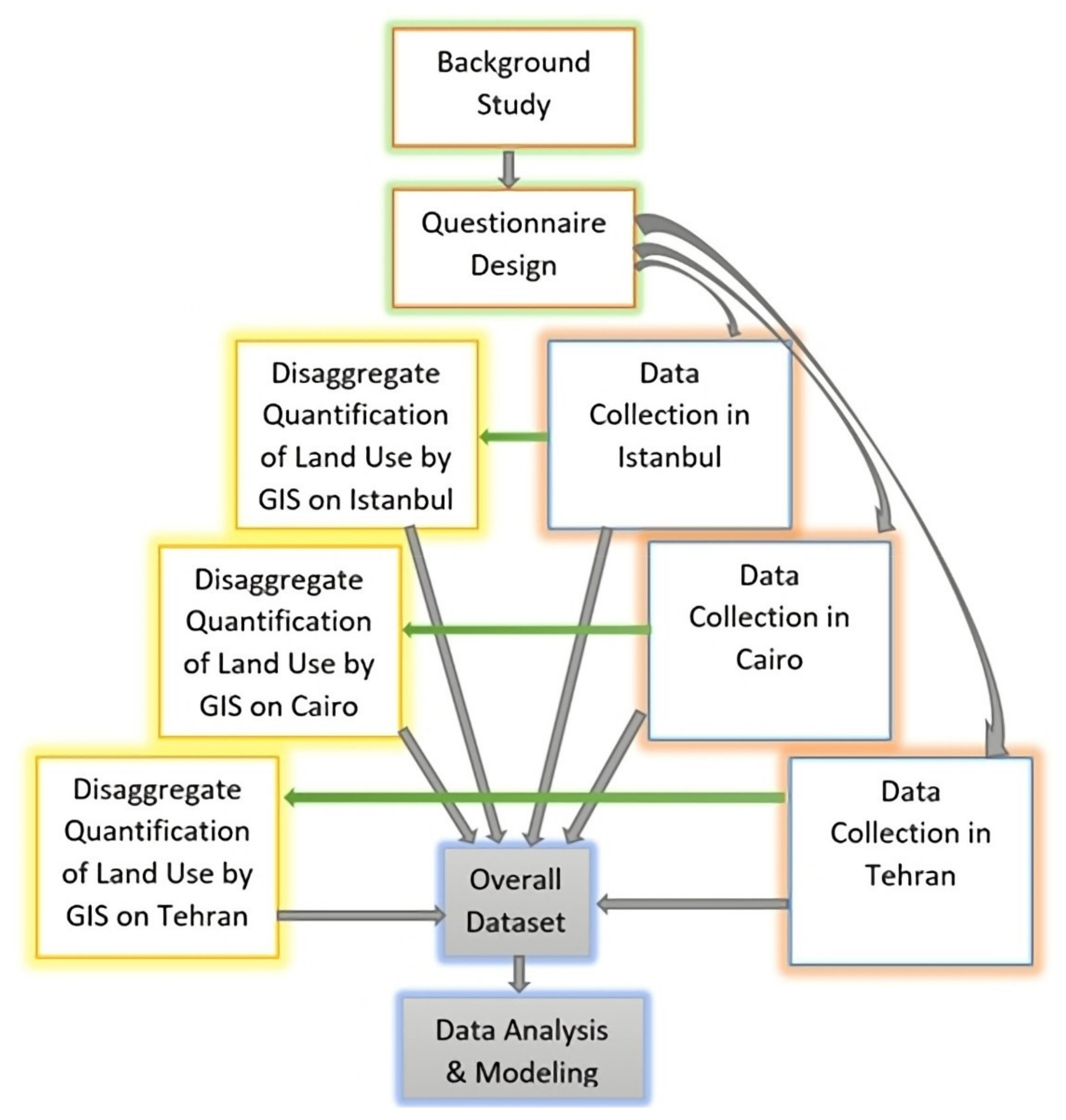
There are two other important variables that are examined in this paper, namely the time passed from the last relocation and daily commuting distance. For the former, the respondents were asked to provide one number in response to the question “how many years ago did your household move to the current home?” In order to quantify the commuting distance, interviewees were asked about the nearest location, landmark, or intersection to their home place and work/study place. It was designed in this way to not violate their privacy. Then, the interviewers marked their living and working places on maps and transferred to ArcGIS by pinpointing on Google Earth first. One-way daily commuting distances were estimated by ArcGIS based on the street networks of the three cities. The commute distances as well as land use variables were all quantified by the study team using ArcGIS in a 600 m catchment area around their homes. This data was connected to the data extracted from the questionnaire for each subject. Thus, a unique dataset was generated for data coming from the survey instrument and the land use quantification. Figure 1 shows how the generation of land use variables by GIS was integrated into the data collection and other methodological sections of the work, such as background studies, questionnaire design, generation of an overall dataset, and statistical analysis.
2.3. Analysis Methods
Out of 8284 interviewees, 4779 respondents answered the related question about residential self-selection, and therefore this number reflects the sample size taken for modeling the determinants of location choices (research question 1). The mobility factors included three options in the original variable that included eight choices. Thus, this sample size was the basis of examining the location choices. In order to answer the first research question of this study, the residential location choice variable was transformed into a dummy (binary) variable with two options: other factors (coded 0) and mobility factors (coded 1). These were: (b) the house was near to my workplace/school, (g) the house was easy for me to commute to my workplace/school, and (h) public transportation is available around the neighborhood. The rest of the options were considered as non-mobility issues. For the modeling of this variable, probit regression modelling was applied with the mentioned variable as the dependent variable. The variables listed in Appendix A were taken as independent variables.
The mobility factors were set as a reference category, so the variables and their categories (if any) were compared with reference to this choice. The model was rerun and the variables with highest p-values were eliminated from the model. The first variables to be eliminated from the model were the ones with the highest p-values. After 16 iterations, eight categorical and continuous variables were kept in the model and it was considered as the best possible model. The following variables were eliminated from the model: intersection density, link-node ratio, cycling, household income, gender, shopping-entertainment place, individual driving license, household car ownership, availability of attractive shopping centers, entertainment place, sense of belonging, frequency of commute trips, activity, subjective security of public transportation use, and shopping-entertainment mode choice inside the neighborhood. The final variables were shopping-entertainment mode, choice outside the neighborhood, frequency of public transit trips, neighborhood attractiveness perception, age, number of driving licenses in household, commuting distance, number of accessed facilities, and accessibility of facilities. Table 1 summarizes the frequencies of the categorical variables of the model and Table 2 shows the descriptive statistics of the continuous variables.
The second and third research questions of this paper seek associations between a dummy variable (residential self-selection) and two continuous variables (commuting distance and the time of the last relocation) separately. For testing the hypothesis of existence of difference in commuting distance and the time passing from the last relocation according to the residential self-selections, the Mann–Whitney U-test was applied, where p-values of less than 0.05 rejected the hypothesis of existence of similarity between the commuting distance and relocation time of those who selected their house location based on mobility and other factors. This nonparametric test of difference was applied because the two continuous variables were non-normal.
In order to check for correlations, it was necessary to break the continuous variables into two groups, one with lower values and one with higher values. In other words, it was needed to find the cutoff point at which a value change occurs, i.e., a point at which the mean commuting distances are significantly different for the two groups of residential location choices or the point at which the time passed from the last relocation is significantly different for the two mentioned groups. For defining these two cutoff points for daily commuting distance and the time of the last relocation, Receiver Operating Characteristic (ROC) curves for the two continuous variables were estimated. The ROC curves modeled the diagnostic ability of residential location choice, as its discrimination threshold is varied. These curves are the summary of four combined conditions (true positive (TP), true negative (TN), false positive (FP), false negative (FN)), which are based on two main conditions: positive (P: the number of real positive cases in the data) and negative (N: the number of real negative cases in the data). These conditions are estimated for all values of the continuous variables versus the binary variable based on a two-axis diagram with the true positive rate named as sensitivity on the vertical axis and false positive rate called 1-specificity. The ROC curve provides the best prediction capability when the area under the curve (AUC) is as high as 100% of the diagram area; in other words, the sensitivity of the continuous variable reaches 1. This happens under perfect conditions—which do not happen in real world applications—but normally an AUC of 90%, 80%, and 70% are excellent, good, and average models. However, in the case of the ROC curves of this study, the highest prediction power of the model was not sought; instead, it was intended to find the cutoff point. For finding the cutoff point, the nearest point on the curve with the shortest distance to the point in the top-left of the diagram (sensitivity = 1) is theoretically the cutoff point. This point can be found using the outputs of the SPSS software, in which the sensitivity and 1-specificity values were provided for each point on the curve. The shortest distance was calculated using Formula (1).
Shortest distance to sensitivity of 1 = √((1 − Sensitivity) 2 + (1 − Specificity) 2)
The Youden Index helps find the exact value of the cutoff point by means of Formula (2):
Youden Index = Sensitivity + Specificity − 1
The value of the Youden Index is useful for finding the exact amount of the point that has the highest sensitivity and specificity at the same time, which will be the cutoff point. The theoretical range of the Youden Index is from −1 to 1, but the practical range in use is from 0 to 1 since negative values of the Youden Index do not have a physical meaning [28]. Therefore, negative values of the Youden Index were omitted here and the related amount of the continuous variables were found for the two continuous variables.
The second step for finding the difference between commuting distance and the time passed from the last relocation for residential location choices was to compute the two continuous variables into two dummy variables using the cutoff points estimated by the ROC curves. The cutoff points were used to break these two variables from the turning points, resulting in finding a significant difference. The results of the Kolmogorov–Smirnov test show that the two continuous variables are non-normal (p < 0.001), thus, for finding the differences of values of the two continuous variables for residential location choice (other factors and mobility factors), the Kruskal–Wallis test was applied, whereas p-values of less than 0.05 indicated a significant change. In case a significant change between high and low values of the continuous variables was found, a significant association between residential location choice and the continuous variable was concluded.
3. Findings
3.1. The Determinants of Residential Location Choices
The results of the binary probit model are summarized in Table 3. All of the variables kept in the model are significant at 0.001 or 0.01 levels, but as expected, the categories of the three categorical variables show different behaviors. In case of the categorical variables, the model compares the likelihood of occurrence of each category of independent variables to a reference category of the same variable regarding mobility reasons (coded 1) to other reasons (coded 0). The categories of shopping-entertainment mode choice outside the neighborhood (in places far away from home) have been compared to using ridesourcing technologies such as taxi apps. An important finding is that individuals who walk for shopping and entertainment purposes to far-away places are 57% less likely to move their house for mobility reasons compared to those who use ridesourcing technologies for the same purpose. However, those who use motorbikes are 62% more likely to relocate for mobility reasons compared to ridesourcing users.
The next significant variable is frequency of public transport ridership with the reference category of rare public transport use. According to the model, respondents who use public transit everyday are 37% more likely to relocate because of mobility reasons compared to people who use public transit rarely. Likewise, people who use public transport a few times per month are 25% more likely to do so compared to rare public transport users.
Neighborhood attractiveness perception is the next significant variable in the model. The reference category is perceiving the neighborhood as very attractive. People who find their neighborhood acceptably attractive and not so attractive are 32% and 34%, respectively, more likely to move house because of mobility reasons compared to those who find their neighborhood very attractive. This means that individuals who have relocated because of transportation reasons find their neighborhood less attractive.
The next five variables in the model are continuous, the first of which is age. Older people are less likely to have moved house because of transportation reasons such as commuting to work. Accordingly, younger generations choose their residential place based on transport needs more than older people. A 10-year increase in age is associated with a 7% decrease in likelihood of moving house because of better mobility. Number of driving licenses in the household is negatively associated with moving house for mobility. One km increase in commuting distances may lead to 4% increase in the chance of moving house for better transportation and commuting. Both accessibility to facilities variables are highly significant (p < 0.001). Having one more facility in the 600 m catchment area of the houses is associated with 1% less probability of relocating for mobility reasons. Likewise, people who have longer walking distances to neighborhood facilities around their current home are more likely to have moved house for mobility reasons.
The model test results, including the goodness of fit and omnibus test, show that the model is valid. The proportion of value to degrees of freedom of deviance is less than 1 (0.751), which is a sign of validity for the model. The likelihood ratio chi-square based on the omnibus test is equal to 306.2 and therefore highly significant (Table 4).
3.2. Association of Residential Location Choice with the Last Relocation Time and Daily Commuting Distance
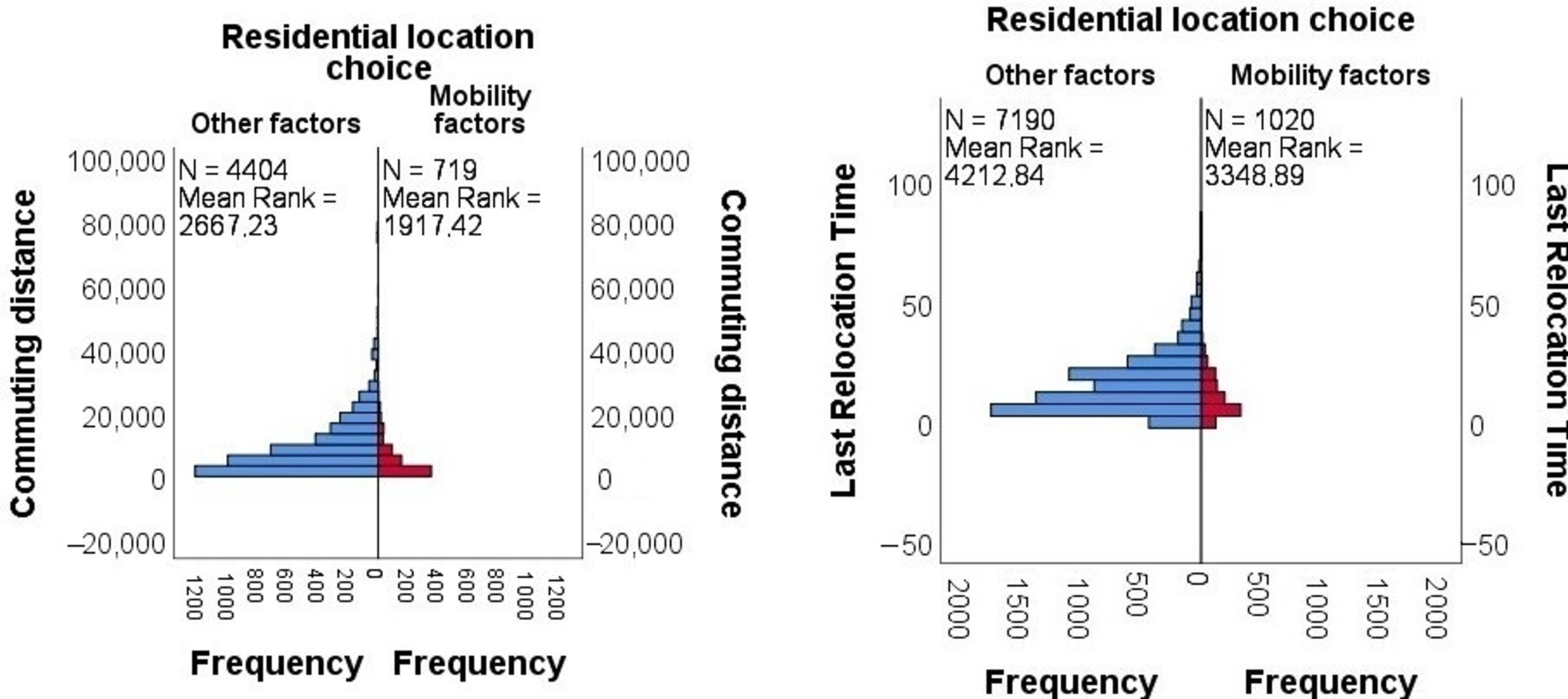
The results of the Mann–Whitney U-test show that the mean rank of commuting distances (continuous) as well as the relocation time (continuous) of people with different residential mobility (mobility vs. others) are significantly different (p < 0.001) (see Figure 2). The findings clearly indicate that the commuting distances of individuals living in households, who have selected their house place based on mobility reasons, commute shorter distances and have relocated to their current home in more recent years. However, these results do not show the turning point in commuting distance and last relocation time when the difference in residential location occurs. Thus, further investigations are necessary.
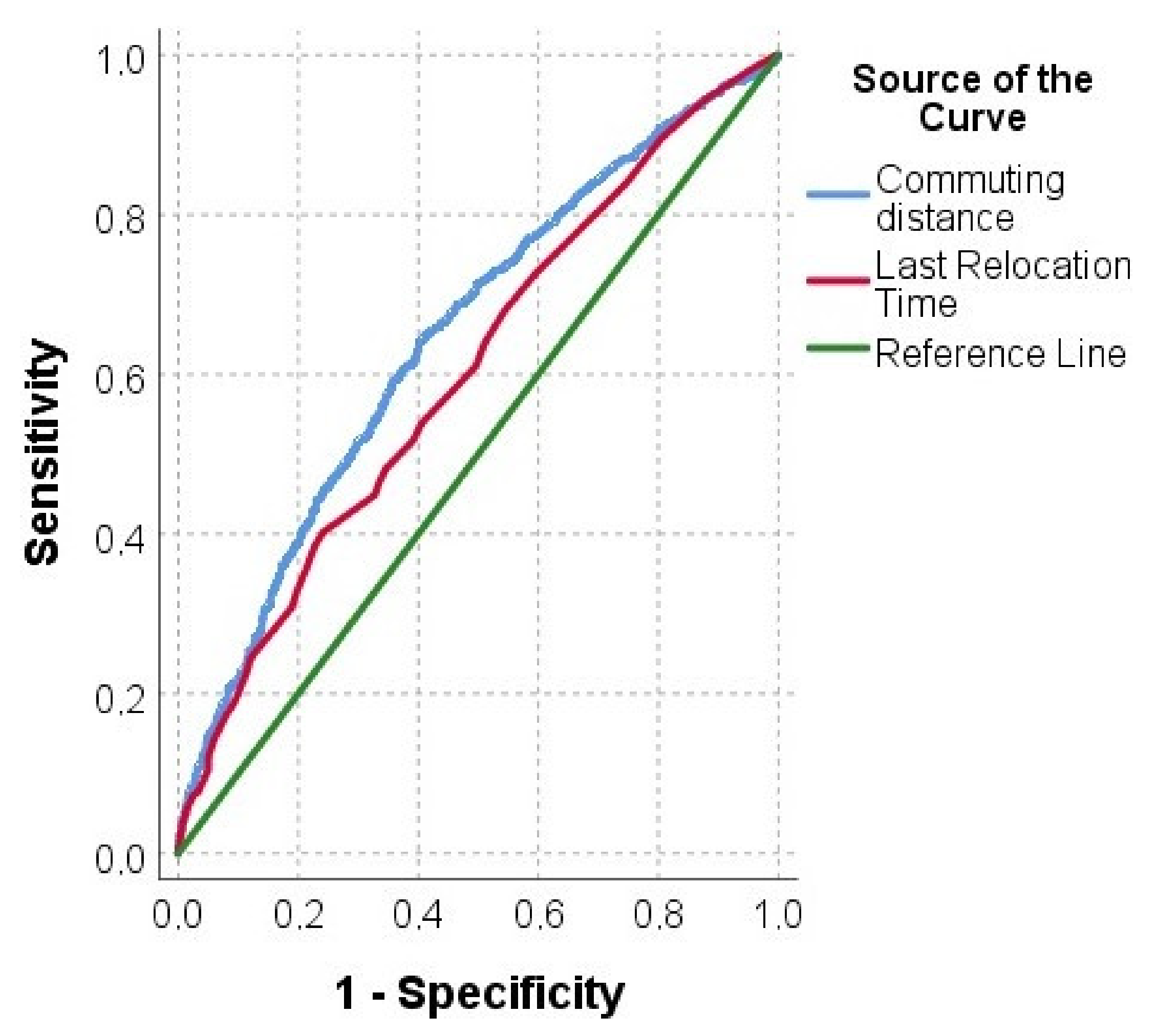
In order to find the association between the abovementioned continuous variables and one-way commuting distance based on street network, the cutoff points where a change in the commuting distance happened were sought by use of ROC curves. The results are shown in Figure 3. The area under the ROC curve (AUC) of commuting distance is 64.7% (p < 0.001) and that of the last relocation time is 60.3% (p < 0.001), whereas the null hypothesis is that the true area of other factors is 0.5. According to these curves, the Youden Index of commuting distance is 0.2392 and that of the last relocation is 0.1612. These values define the cutoff points of 4.298 km for commuting distance and 15.5 years passing from the last house relocation.
In order to test the validity of these cutoff values, the chi-square test of independence was applied to commuting distances with values more than or less than 4.298 km on the one side and the dummy variable of residential location choice (mobility vs. other reasons) on the other side. As seen in Table 5, the test results show a significant difference between the commuting distances of the two groups (p < 0.001). This difference is caused by the association between residential location choice and commuting distance. When the residential location decisions change from mobility-oriented to other reasons, commuting distances increase. This means that 719 individuals out of 5123 who commute less than a one-way distance of 4.298 km declared that their household chose their home location based on mobility. That is equal to 14%, and this figure is lower for those who reported choosing their location based on other reasons, 9.6%. This shows a significant difference between these two groups. In Table 6, the number of subjects with a value for commuting distance is higher than the 4779 respondents who reported about their house location choice, because the number of interviewees who gave information on their commute distance was higher.
Similarly, an association between the time passed from the last relocation and residential self-selection was detected. There is a significant difference in the reasons of newer relocations compared to older ones. Older relocations were less based on mobility reasons. More than 15.2% of the respondents who moved house less than 15.5 years ago reported to have done so based on mobility or commuting reasons, while this figure is 8% for those who moved house more than 15.5 years ago (Table 6). This significant difference (p < 0.001) shows that the attitudes and preferences of people regarding home location and mobility have changed in the last 15.5 years before the time of the survey of this study (2017). Here, more people reported on the time of their last relocation compared to those who answered the location choice question.
4. Discussion
The results of the binary probit model of this study find age to be important in defining residential self-selection. Some of the findings of the model contradict the findings in high-income countries. For instance, the current study did not find any significant relation between location self-selections and car ownership, while in the Netherlands, this relation has been found to be important [29]. In MENA cities, young people are more likely to choose their home location based on mobility needs, while older urban dwellers prioritize other factors. It has been found that in Nanjing, China, residential self-selection influences on travel behavior are different among the elderly (60+ years old) and younger respondents (18–59 years old) [30]. This is in line with the findings of this study. China is considered to be an emerging market or, in some definitions, a developing country. In this specific case, the behaviors in the MENA region are similar to those in China. Moreover, in several Western studies, income has been found to be relevant in location decision [31,32,33,34], while in the model of this study, household monthly income was omitted from the model as it was not significant.
A very important issue that the current study raises is the importance of accessibility to local amenities, including the number of such facilities around homes and the walking distances to them. In the model developed in this study, these variables are highly significant. This finding is consistent with the conclusions of a recent study conducted by Baraklianos et al. (2020), who found accessibility factors to be of importance in their residential location choice model in the Lyon metropolitan area in France [35]. The relations between residential location choice and accessibility of work place and different types of services have also been shown in the Stockholm region, Sweden [36], though in this model, Eliasson did not categorize the location choices into mobility and non-mobility. The study also confirms the findings of Lee et al. (2010) which showed relations between location choices and cumulative opportunities for shopping in the Puget Sound region, USA [37], as well as the findings of Guo (2004) about the importance of accessibility of shopping opportunities in the Dallas/Fort Worth metroplex, USA [38], and finally the results of Zhang and Guhathakurta (2018), who found higher number of amenities to be important in Atlanta, USA [39]. However, at the same time, the results reject the findings of some of the studies that did not recognize accessibility as a key factor in house location choices in Chicago, USA [40], Melbourne, Australia [41], and Santander, Spain [42].
The findings of the current study regarding strong correlations of commuting distance with residential location choices are in line with the findings of Blijie in the Dutch context [29]. The present study shows that the current commuting distance is in relation with the last relocation choice. This can also be compared to the findings of Chen et al. (2008), who found this relation between the prior commute distance and the last relocation in the Puget Sound region, USA [43], as well as the work of Cockx and Canters (2020) which showed the effect of job accessibility on residential self-selection in Belgium [44]. In general, the MENA findings show that the trade-off between mobility motives and other factors is becoming more serious in the large cities of the region, as it has already been shown that in the Western context, the subjective value of time as a component of commuting is compared to the household’s willingness to pay by rent to reduce commuting time [45].
According to Fatmi and Habib (2017), individuals prefer to persist with their past commute mode [46]. In this regard, the study on the MENA region shows that longer commuting distances in large cities and agglomerations might change the attitudes to changing house location. This change can theoretically happen in commuting distances of more than 8596 m as a threshold. Long commuting distances in weaved streets with high traffic congestion of such cities might encourage younger generations to live in the vicinity of their work/study places. The results of the statistical model of this paper as well as the hypothesis testing confirm this. Individuals who moved house less than 15.5 years ago have done so more strongly than those who moved earlier. This reflects a change in the lifestyles of people living in large cities. These findings are generalizable to up to 27 cities, each accommodating at least one million people, according to a recent study [47]. The change in the attitudes of younger generations strengthens the ties between residential self-selection with urban travel behavior in the region. On one hand, it adds to the complexity of the factors influencing travel demand; on the other hand, it can be used for local urban and transportation planners as a basis for policymaking. For instance, based on the findings of this paper, it is clear that in the case of availability of employment centers and jobs less than four kilometers distance from the living places and residents, people consider this a proper commuting distance. It has been shown in this paper that people who have chosen their living location based on mobility preferences live in places as near as 4298 m to their working place.
This finding is related to the question asked by De Vos and Witlox: “Do people live in urban neighborhoods because they do not like to travel?” [48]. The response of this study is yes, but it might be related to the attitudes and perceptions of people. If commuting is so important to them that they choose their house location based on it, then they are likely to choose a location of less than 4.3 km distance to the workplace of one of the most frequently commuting household members. This assumption, which is largely suggested by this study, can be adopted for urban planning policymaking by providing employment clusters in less dense areas of cities or the metropolitan regions that are aimed to attract more residents in the future, with the purpose of defining the development orientation of the city. Of course, this paper can only suggest this strategy for the larger cities of the MENA region, since it is backed only by empirical findings of this region.
Another input of this study to urban planning and housing policy is that cheaper, social, or affordable housing can be targeted by urban development plans on the periphery of the large cities, if employment has been already thought of. This study shows that younger generations may give more importance to commuting in choosing their house location compared to previous generations. Thus, urban policymakers can attract them to new quarters only if there are working opportunities nearby. This is linked to studies that suggest providing jobs with the purpose of turning urban sprawl from a problem to an opportunity, i.e., making commuting travels shorter [49,50]. Of course, this strategy is not suitable for medium-sized or small cities in the region, as one cannot assume that residents would choose commuting necessities over socioeconomic motives without empirical results.
These planning opportunities can improve the reciprocal functions of land use and transport behavior. On one hand, urban growth can be controlled, while on the other hand, travel behavior can be directed towards more sustainable and perhaps more active modes. The previous urban planning studies have shown that in Egypt and Iran, a lack, deficiency, or absence of urban development plans have led to urban sprawl [51]. Utilizing land use–transportation integrated planning can ease some of the long-lasting problems of cities like Tehran, Istanbul, and Cairo in urban travels, such as traffic congestion, long commuting, and transport-related environmental pollutions as well as urban sprawl and its negative social and financial impacts. From this perspective, this study is in line with the approach of Western solutions of the past four decades.
5. Conclusions
The present study sheds light on the determinants of residential location choice in the less-studied context of the MENA region and at the same time finds some of the contextual differences with these determinants in high-income and mostly Western countries. The eight variables of shopping-entertainment mode choice outside the neighborhood (in faraway places), frequency of public transit trips, neighborhood attractiveness perception, age, number of driving license in household, commuting distance, number of accessed facilities, and the (walkable) accessibility to facilities have been recognized to influence residential self-selections. Moreover, it has been found that people who have chosen their current home based on mobility commute a daily mean distance of 8596 m, while those who chose their home based on other reasons such as socioeconomics or personal reasons commute longer. Finally, people whose location choice is based on transportation reasons are likely to have moved to their new home less than 15.5 years ago, while those who moved before that date likely had other reasons. This shows how the attitudes of people towards residential location have changed in the MENA region. Such findings are of importance from a basic scientific point of view; at the same time, decision makers and urban planners can use them for the purpose of making commuting more sustainable.
Although the sample size of this study is enough for providing the necessary power for the analyses, this study has its own limitations, e.g., the role of the personal life events in choosing house locations was not investigated by this study. Life-course events such as completing school or university studies, marriage, starting a new job, having a child, etc. may significantly affect the location choices. These correlations were not investigated here, because this study was primarily designed not only to examine the housing preferences, but also to investigate the travel behaviors in the three cities. In the future, in studies that are fundamentally designed for the purpose of studying housing and relocation tendencies, the investigation of the relations between residential self-selection and “mobility biographies” in the MENA region will be intriguing.
Author Contributions
Conceptualization, methodology, resources and data, formal analysis, writing—original draft preparation, writing—reviewing and editing: H.M. The author has read and agreed to the published version of the manuscript.
Funding
This study was undertaken with the support of German Research Foundation (DGF) as the research project “Urban Travel Behavior in Large Cities of MENA Region” (UTB-MENA) with the project number MA6412/3-1.
Institutional Review Board Statement
Ethical review and approval were waived for this study.
Informed Consent Statement
Written informed consent has not been obtained from the respondents of the interviews of this study, due to the cultural and socio-political conditions of the countries, in which data were collected.
Data Availability Statement
The data have been collected using public funds but at the time of the publication of this paper, it has not been shared on a repository.
Acknowledgments
I acknowledge support by the German Research Foundation and the Open Access Publication Fund of Technische Universität Berlin.
Conflicts of Interest
The author declares no conflict of interest. The funders had no role in the design of the study; in the collection, analyses, or interpretation of data; in the writing of the manuscript, or in the decision to publish the results.
Appendix A

Table A1.
Quantification methods of the dependent and independent variables of this study (source for land use variables: [27]; for other variables: [52,53]).
| Variable Type for Modeling Purpose | Variable | Data Type | Unit | Description |
|---|---|---|---|---|
| Main Target Variables or Independent Variables | Residential Location Choice | Binary | - | Other factors: (Code: 0) (a) the house was affordable to buy or rent, (c) the surrounding environment is attractive, (d) the house will have higher price in the future, (e) to be near to our relatives and/or friends, and (f) I live here since I was born/my childhood, Mobility Factors: (Code: 1) (b) the house was near to my working place/school, (g) the house was easy for me to commute to my working place/school, and finally, (h) public transportation is available around the neighborhood. |
| Last Relocation Time | Continuous | Year | The number of years passed from the last residential relocation of the respondent and possibly his/her family. | |
| Commuting Distance | Continuous | Km | The street network-based distance from home to respondents’ workplace, who have work/study activity, was estimated by the information about the place of home in the neighborhood as well as the workplace obtained from questionnaires. | |
| Independent | Gender | Binary | - | Male or female (“other” was not applied due to cultural considerations). |
| Age | Continuous | Year | Reported age of the respondent. | |
| Individual Driving License Ownership | Binary | - | Possession of a driving license by the respondent: yes or no. | |
| Activity | Binary | - | Work/study or no work/study. | |
| Household Car Ownership | Continuous | - | The number of personal cars possessed by family members. | |
| No. of Driving License in Household | Continuous | - | The number of family members who possess a driving license. | |
| Household Income | Continuous | Euro | Reported gross household monthly income converted from Rial (Toman), Turkish Lira, and Egyptian Pound to Euro in summer and autumn of 2017. | |
| Entertainment Place | Binary | - | The place the respondent usually has his/her entertainment and leisure activities: inside the neighborhood or farther. | |
| Shopping-Entertainment Mode Choice in Neighborhood | Categorical | - | The place of the respondent’s shopping or recreational activities inside the neighborhood: on foot, bicycle, motorbike, taxi, taxi apps, informal public transport, personal/household car, others, bus/minibus/metrobus/ microbus/BRT/van, metro/light rail train/tram, organizational service/shuttle. | |
| Shopping-Entertainment Mode Choice outside Neighborhood | Categorical | - | The place of the respondent’s shopping or recreational activities outside the neighborhood: on foot, bicycle, motorbike, taxi, taxi apps, informal public transport, personal/household car, others, bus/minibus/metrobus /microbus/BRT/van, metro/light rail train/tram, and organizational service/shuttle. | |
| Frequency of Public Transit Trips | Categorical | - | The usual frequency of the respondent’s public transportation ridership according to him/her: every day, a few times per week, a few times per month, rarely, almost never. | |
| Cycling | Binary | - | Cycling to near destinations inside the neighborhood: yes or no. | |
| Attractive Shopping Centers in Neighborhood | Binary | - | Presence of attractive shops or shopping centers in the neighborhood of the respondent according to him/her: yes or no. | |
| Subjective Security of Public Transport | Categorical | - | The level of the securing of public transportation according to the respondent’s perception: very secure, secure, medium, insecure, and very insecure. | |
| Sense of Belonging to Neighborhood | Binary | - | Respondent’s perception about his/her sense of belonging to the neighborhood: yes or no. | |
| Neighborhood Attractiveness Perception | Categorical | - | Perception of the respondent regarding the attractiveness of the neighborhood social/recreational facilities: very attractive, acceptably attractive, medium, little attractive, and not attractive or not available. | |
| Frequency of Commute Trips | Continuous | - | The number of commute trips of the respondent during the past 7 days. | |
| Intersection Density | Continuous | Intersections/ha | The number of intersections per hectare in a 600 m catchment area (based on the network) of each of the respondents’ homes. Calculations were conducted for areas inside the neighborhood boundary or outside. | |
| Link-Node Ratio | Continuous | - | The number of links (street segments) divided by nodes (street intersections) of the street network within a 600 m catchment area (based on the network) of each of the respondents’ homes. Calculations were conducted for areas inside the neighborhood boundary or outside. This indicator evaluates the typology of intersections (i.e., four- and five-ways intersections obtain higher values than three-way intersections). Values of 1.4 and higher indicate good connectivity. | |
| Street Length Density | Continuous | M/ha | The length of streets divided by the area of the 600 m catchment area (based on the network) of the respondents’ homes. Calculations were conducted for areas inside the neighborhood boundary or outside. Higher densities indicate better connectivity. | |
| No. of Accessed Facilities | Continuous | - | The number of neighborhood public facilities within a 600 m catchment area (based on the network) of the respondents’ homes. The facilities included five types: bakeries, clinics and other medical centers, mosques, parks, and schools. | |
| Accessibility to Facilities | Continuous | Meter | The average distance (based on the network) from each respondent’s home to neighborhood public facilities within the neighborhood or located within a linear 600 m buffer outside the neighborhood boundary. The facilities included five types: bakeries, clinics and other medical centers, mosques, parks, and schools. |
References
- Cao, X.; Mokhtarian, P.L.; Handy, S.L. Examining the impacts of residential self-selection on travel behaviour: A focus on empirical findings. Transp. Rev. 2009, 29, 359–395. [Google Scholar] [CrossRef]
- Li, T.; Sun, H.; Wu, J.; Lee, D.-H. Household residential location choice equilibrium model based on reference-dependent theory. J. Urban Plan. Dev. 2020, 146, 4019024. [Google Scholar] [CrossRef]
- Bohte, W.; Maat, K.; van Wee, B. Residential Self-Selection. The Effect of Travel-Related Attitudes and Lifestyle Orientation on Residential Location Choice; Evidence from the Netherlands. In Proceedings of the 11th World Conference on Transport Research World Conference on Transport Research Society, University Berkeley, Berkeley, CA, USA, 24–28 June 2007. [Google Scholar]
- Habib, M.A.; Miller, E.J. Reference-Dependent Residential Location Choice Model within a Relocation Context. Transp. Res. Rec. 2009, 2133, 92–99. [Google Scholar] [CrossRef]
- Xue, F.; Yao, E.; Jin, F. Exploring residential relocation behavior for families with workers and students; A study from Beijing, China. J. Transp. Geogr. 2020, 89, 102893. [Google Scholar] [CrossRef]
- Kim, J.H.; Pagliara, F.; Preston, J. The Intention to Move and Residential Location Choice Behaviour. Urban Stud. 2005, 42, 1621–1636. [Google Scholar] [CrossRef]
- Zhou, B.; Kockelman, K.M. Microsimulation of residential land development and household location choices: Bidding for land in Austin, Texas. Transp. Res. Rec. 2008, 2077, 106–112. [Google Scholar] [CrossRef] [Green Version]
- Bürgle, M. Residential location choice model for the Greater Zurich area: Conference paper STRC 2006. In Proceedings of the 6th Swiss Transport Research Conference, Ascona, Switzerland, 15–17 March 2006; Volume 359. [Google Scholar]
- Heinen, E.; van Wee, B.; Panter, J.; Mackett, R.; Ogilvie, D. Residential self-selection in quasi-experimental and natural experimental studies: An extended conceptualization of the relationship between the built environment and travel behavior. J. Transp. Land Use 2018, 11, 11. [Google Scholar] [CrossRef] [Green Version]
- Ettema, D.; Nieuwenhuis, R. Residential self-selection and travel behaviour: What are the effects of attitudes, reasons for location choice and the built environment? J. Transp. Geogr. 2017, 59, 146–155. [Google Scholar] [CrossRef]
- Scheiner, J. Residential self-selection in travel behavior: Towards an integration into mobility biographies. J. Transp. Land Use 2014, 7, 15. [Google Scholar] [CrossRef] [Green Version]
- Boone-Heinonen, J.; Guilkey, D.K.; Evenson, K.R.; Gordon-Larsen, P. Residential self-selection bias in the estimation of built environment effects on physical activity between adolescence and young adulthood. Int. J. Behav. Nutr. Phys. Act. 2010, 7, 70. [Google Scholar] [CrossRef] [Green Version]
- Cao, J. Residential self-selection in the relationships between the built environment and travel behavior: Introduction to the special issue. J. Transp. Land Use 2014, 7, 1. [Google Scholar] [CrossRef] [Green Version]
- Næss, P. Residential Self-Selection and Appropriate Control Variables in Land Use: Travel Studies. Transp. Rev. 2009, 29, 293–324. [Google Scholar] [CrossRef]
- Masoumi, H.E. Residential self-selection and its effects on urban commute travels in Iranian cities compared to US, UK, and Germany. Int. J. Soc. Sci. 2013, 7, 877–881. [Google Scholar]
- Masoumi, H.; Ibrahim, M.R.; Aslam, A.B. The Relation Between Residential Self-Selection and Urban Mobility in Middle Eastern Cities: The Case of Alexandria, Egypt. Urban Forum. 2021, 1–27. [Google Scholar] [CrossRef]
- Ibrahim, M.R.; Masoumi, H.E. Will Distance to the Capital City Matter When Supplying New Cities in Egypt? GeoScape 2016, 10, 35–52. [Google Scholar] [CrossRef] [Green Version]
- Mehriar, M.; Masoumi, H.; Mohino, I. Urban Sprawl, Socioeconomic Features, and Travel Patterns in Middle East Countries: A Case Study in Iran. Sustainability 2020, 12, 9620. [Google Scholar] [CrossRef]
- Al Khalili, S.M.S. Modelling of Optimal Place for Living in United Aarab Emirates Using Geographical Information System; Universiti Teknologi Malaysia Institutional Repository: Johor, Malaysia, 2013. [Google Scholar]
- Aslam, A.B.; Masoumi, H.E.; Naeem, N.; Ahmad, M. Residential location choices and the role of mobility, socioeconomics, and land use in Hafizabad, Pakistan. Urbani Izziv 2019, 30, 115–128. [Google Scholar] [CrossRef]
- Rehman, A.; Jamil, F. Impact of urban residential location choice on housing, travel demands and associated costs: Comparative analysis with empirical evidence from Pakistan. Transp. Res. Interdiscip. Perspect. 2021, 10, 100357. [Google Scholar]
- Digambar, A.P.; Mazumder, T. Residential location choice: A study of household preferences for the city of Nagpur. Inst. Town Plan. India J. 2010, 7, 1–19. [Google Scholar]
- Shrivastava, A. Assessment of residential location choice behaviour in Bhopal city. Ph.D. Thesis, School of planning and architecture, SPA, Bhopal, India, 2015. [Google Scholar]
- Munshi, T. Built environment and mode choice relationship for commute travel in the city of Rajkot, India. Transp. Res. Part D Transp. Environ. 2016, 44, 239–253. [Google Scholar] [CrossRef]
- Reddi, A.S. Importance of Metro and Bus Service Availability in Residential Location Choice and Mode Choice. Ph.D. Thesis, Indian Institute of Technology, Kharagpur, India, 2015. [Google Scholar]
- De Vos, J.; Alemi, F. Are young adults car-loving urbanites? Comparing young and older adults’ residential location choice, travel behavior and attitudes. Transp. Res. Part A Policy Pr. 2020, 132, 986–998. [Google Scholar] [CrossRef]
- Masoumi, H.; Gouda, A.A.; Layritz, L.; Stendera, P.; Matta, C.; Tabbakh, H.; Fruth, E. Urban Travel Behavior in Large Cities of MENA Region: Survey Results of Cairo, Istanbul, and Tehran. In Center for Technology and Society; ADL: New York, NY, USA, 2018. [Google Scholar]
- Shan, G. Improved Confidence Intervals for the Youden Index. PLoS ONE 2015, 10, e0127272. [Google Scholar] [CrossRef] [PubMed] [Green Version]
- Blijie, B. The impact of accessibility on residential choice-empirical results of a discrete choice model. In Proceedings of the 45th Congress of the European Regional Science Association: “Land Use and Water Management in a Sustainable Network Society”, Amsterdam, The Netherlands, 23–27 August 2005. [Google Scholar]
- Cheng, L.; De Vos, J.; Shi, K.; Yang, M.; Chen, X.; Witlox, F. Do residential location effects on travel behavior differ between the elderly and younger adults? Transp. Res. Part D Transp. Environ. 2019, 73, 367–380. [Google Scholar] [CrossRef]
- Zondag, B.; Pieters, M. Influence of accessibility on residential location choice. Transp. Res. Rec. 2005, 1902, 63–70. [Google Scholar] [CrossRef]
- Waddell, P. Reconciling household residential location choices and neighborhood dynamics. In Under Revision, Sociological Meth-Ods and Research; Evans School of Public Affairs: Seattle, DC, USA, 2006. [Google Scholar]
- Guo, J.Y.; Bhat, C.R. Operationalizing the concept of neighborhood: Application to residential location choice analysis. J. Transp. Geogr. 2007, 15, 31–45. [Google Scholar] [CrossRef] [Green Version]
- Pinjari, A.R.; Bhat, C.R.; Hensher, D.A. Residential self-selection effects in an activity time-use behavior model. Transp. Res. Part B Methodol. 2009, 43, 729–748. [Google Scholar] [CrossRef] [Green Version]
- Baraklianos, I.; Bouzouina, L.; Bonnel, P.; Aissaoui, H. Does the accessibility measure influence the results of residential location choice modelling? Transportation 2020, 47, 1147–1176. [Google Scholar] [CrossRef] [Green Version]
- Eliasson, J. The influence of accessibility on residential location. In Residential Location Choice; Springer: Berlin/Heidelberg, Germany, 2010; pp. 137–164. [Google Scholar]
- Lee, B.H.Y.; Waddell, P.; Wang, L.; Pendyala, R.M. Reexamining the influence of work and nonwork accessibility on residential location choices with a microanalytic framework. Environ. Plan. A 2010, 42, 913–930. [Google Scholar] [CrossRef] [Green Version]
- Guo, J.Y. Addressing Spatial Complexities in Residential Location Choice Models. Ph.D Thesis, The University of Texas at Austin, Austin, TX, USA, 2004. [Google Scholar]
- Zhang, W.; Guhathakurta, S. Residential Location Choice in the Era of Shared Autonomous Vehicles. J. Plan. Educ. Res. 2021, 41, 135–148. [Google Scholar] [CrossRef] [Green Version]
- Hu, L.; Wang, L. Housing location choices of the poor: Does access to jobs matter? Hous. Stud. 2019, 34, 1721–1745. [Google Scholar] [CrossRef]
- Saghapour, T.; Moridpour, S. The role of neighbourhoods accessibility in residential mobility. Cities 2019, 87, 1–9. [Google Scholar] [CrossRef]
- Ibeas, Á.; Cordera, R.; dell’Olio, L.; Coppola, P. Modelling the spatial interactions between workplace and residential location. Transp. Res. Part A Policy Pract. 2013, 49, 110–122. [Google Scholar] [CrossRef] [Green Version]
- Chen, J.; Chen, C.; Timmermans, H.J.P. Accessibility trade-offs in household residential location decisions. Transp. Res. Rec. 2008, 2077, 71–79. [Google Scholar] [CrossRef]
- Cockx, K.; Canters, F. Determining heterogeneity of residential location preferences of households in Belgium. Appl. Geogr. 2020, 124, 102271. [Google Scholar] [CrossRef]
- Pérez, P.E.; Martínez, F.J.; Ortúzar, J.d.D. Microeconomic Formulation and Estimation of a Residential Location Choice Model: Implications for the Value of Time. J. Reg. Sci. 2003, 43, 771–789. [Google Scholar] [CrossRef]
- Fatmi, M.R.; Habib, M.A. Modelling mode switch associated with the change of residential location. Travel Behav. Soc. 2017, 9, 21–28. [Google Scholar] [CrossRef]
- Masoumi, H.; Fruth, E. Transferring Urban Mobility Studies in Tehran, Istanbul, and Cairo to Other Large MENA Cities: Steps toward Sustainable Transport. Urban Dev. Issues 2020, 65, 27–44. [Google Scholar] [CrossRef]
- De Vos, J.; Witlox, F. Do people live in urban neighbourhoods because they do not like to travel? Analysing an alternative residential self-selection hypothesis. Travel Behav. Soc. 2016, 4, 29–39. [Google Scholar] [CrossRef] [Green Version]
- Carane, R.; Chapman, D.G. Traffic and Sprawl: Evidence from US Commuting from 1985–1997; University of California: Los Angeles, CA, USA, 2003. [Google Scholar]
- Crane, R.; Chatman, D.G. As jobs sprawl, whither the commute? Access Mag. 2003, 1, 14–19. [Google Scholar]
- Masoumi, H.E.; Hosseini, M.; Gouda, A.A. Drivers of urban sprawl in two large Middle-eastern countries: Literature on Iran and Egypt. Hum. Geogr. 2018, 12, 55–79. [Google Scholar] [CrossRef]
- Masoumi, H. Urban commute travel distances in Tehran, Istanbul, and Cairo: Weighted least square models. Urban Sci. 2020, 4, 39. [Google Scholar] [CrossRef]
- Masoumi, H.E. A discrete choice analysis of transport mode choice causality and perceived barriers of sustainable mobility in the MENA region. Transp. Policy 2019, 79, 37–53. [Google Scholar] [CrossRef]
Figure 1.
The methodology scheme.

Figure 2.
The difference in commuting distance (left) and last relocation time of people (right) who chose their house location based on mobility vs. other reasons.
Figure 2.
The difference in commuting distance (left) and last relocation time of people (right) who chose their house location based on mobility vs. other reasons.

Figure 3.
The ROC curve of commuting distance and the last relocation time based on the dummy variable of residential location choice (mobility vs. other factors).
Figure 3.
The ROC curve of commuting distance and the last relocation time based on the dummy variable of residential location choice (mobility vs. other factors).

Table 1.
The categorical variables in the probit model and the frequencies of their categories.
| Variable | Category | n | % | |
|---|---|---|---|---|
| Dependent Variable | Residential location choice | Other Factors | 4109 | 86 |
| Mobility Factors | 670 | 14 | ||
| Total | 4779 | 100 | ||
| Factor | Shopping-Entertainment Mode Choice outside Neighborhood | Missing | 19 | 0.4 |
| Bicycle | 10 | 0.2 | ||
| Bus | 1560 | 32.6 | ||
| Informal Public Transport | 128 | 2.7 | ||
| Metro/Light Rail/Tram | 737 | 15.4 | ||
| Motorbike | 119 | 2.5 | ||
| On Foot | 21 | 0.4 | ||
| Personal/Household Car | 1967 | 41.2 | ||
| Service/Shuttle | 12 | 0.3 | ||
| Taxi | 102 | 2.1 | ||
| Taxi Apps | 104 | 2.2 | ||
| Total | 4779 | 100 | ||
| Frequency of Public Transit Trips | Missing | 19 | 0.4 | |
| A Few Times Per Month | 620 | 13.0 | ||
| A Few Times Per Week | 927 | 19.4 | ||
| Almost Never | 221 | 4.6 | ||
| Every Day | 2476 | 51.8 | ||
| Rarely | 516 | 10.8 | ||
| Total | 4779 | 100.0 | ||
| Neighborhood Attractiveness Perception | Missing | 17 | 0.4 | |
| Acceptably Attractive | 1200 | 25.1 | ||
| Little Attractive | 1210 | 25.3 | ||
| Medium | 1545 | 32.3 | ||
| Not Attractive | 641 | 13.4 | ||
| Very Attractive | 166 | 3.5 | ||
| Total | 4779 | 100 | ||
Table 2.
The descriptive statistics of the continuous variables in the probit model.
| Variable | n | Minimum | Maximum | Mean | Std. Deviation |
|---|---|---|---|---|---|
| Age | 4779 | 7 | 75 | 32.99 | 11.3 |
| No. of Driving Licenses in Household | 4779 | 0 | 7 | 1.76 | 1.1 |
| Commuting Distance (Km) | 4779 | ≈0 | 77.106 | 9.14 | 8.8 |
| No. of Accessed Facilities | 4779 | 0 | 55 | 12.68 | 9.4 |
| Accessibility to Facilities (M) | 4779 | 633 | 3497 | 1379.08 | 472.6 |
Table 3.
Binary probit regression model for residential location choice (reference category: mobility factors).
Table 3.
Binary probit regression model for residential location choice (reference category: mobility factors).
| Variable/Category | B | Wald Chi-Square | p | β |
|---|---|---|---|---|
| Intercept | 1.336 | 29.494 | <0.001 | 3.806 |
| Shopping-Entertainment Mode Choice outside Neighborhood = Missing | Non-significant | |||
| Shopping-Entertainment Mode Choice outside Neighborhood = Bicycle | Non-significant | |||
| Shopping-Entertainment Mode Choice outside Neighborhood = Bus | Non-significant | |||
| Shopping-Entertainment Mode Choice outside Neighborhood = Informal public transport | Non-significant | |||
| Shopping-Entertainment Mode Choice outside Neighborhood = Metro/light rail/tram | Non-significant | |||
| Shopping-Entertainment Mode Choice outside Neighborhood = Motorbike | 0.483 | 4.041 | 0.044 | 1.621 |
| Shopping-Entertainment Mode Choice outside Neighborhood = On foot | −0.843 | 6.368 | 0.012 | 0.430 |
| Shopping-Entertainment Mode Choice outside Neighborhood = Personal/household car | Non-significant | |||
| Shopping-Entertainment Mode Choice outside Neighborhood = Service/shuttle | −0.993 | 6.296 | 0.012 | 0.370 |
| Shopping-Entertainment Mode Choice outside Neighborhood = Taxi | Non-significant | |||
| Shopping-Entertainment Mode Choice outside Neighborhood = Taxi apps | Reference Category | |||
| Frequency of Public Transit Trips = Missing | Non-significant | |||
| Frequency of Public Transit Trips = A few times per month | 0.225 | 6.038 | 0.014 | 1.252 |
| Frequency of Public Transit Trips = A few times per week | Non-significant | |||
| Frequency of Public Transit Trips = Almost never | Non-significant | |||
| Frequency of Public Transit Trips = Every day | 0.314 | 14.742 | <0.001 | 1.369 |
| Frequency of Public Transit Trips = Rarely | Reference Category | |||
| Neighborhood Attractiveness Perception = Missing | Non-significant | |||
| Neighborhood Attractiveness Perception = Acceptably attractive | 0.281 | 5.216 | 0.022 | 1.324 |
| Neighborhood Attractiveness Perception = Little attractive | 0.291 | 5.396 | 0.020 | 1.338 |
| Neighborhood Attractiveness Perception = Medium | Non-significant | |||
| Neighborhood Attractiveness Perception = Not attractive | Non-significant | |||
| Neighborhood Attractiveness Perception = Very attractive | Reference Category | |||
| Age | −0.007 | 11.496 | 0.001 | 0.993 |
| No. of Driving License in Household | −0.074 | 9.139 | 0.003 | 0.929 |
| Commuting distance | 0.039 | 98.497 | <0.001 | 1.040 |
| No. of Accessed Facilities | −0.012 | 19.116 | <0.001 | 0.988 |
| Accessibility to Facilities (m) | <0.001 | 14.583 | <0.001 | ≈1.000 |
Table 4.
Validity test for the binary probit regression model of residential location choice.
| Goodness of Fit | |||
|---|---|---|---|
| Value | df | Value/df | |
| Deviance | 3567.8 | 4753 | 0.751 |
| Omnibus Test | |||
| Likelihood Ratio Chi-Square | 306.2 | ||
| Df | 25 | ||
| P | <0.001 | ||
Table 5.
The results of chi-square test of independence between residential location choice (mobility vs. others) and commuting distance (less than or more than 4.298 Km).
Table 5.
The results of chi-square test of independence between residential location choice (mobility vs. others) and commuting distance (less than or more than 4.298 Km).
| Frequencies of Residential Self-Selections and Commuting Distance Categories | ||||
|---|---|---|---|---|
| Residential location choice | Total | |||
| Other factors | Mobility factors | |||
| Commuting Distance 4298 | <4.298 Km | 4404 | 719 | 5123 |
| ≥4.298 Km | 2857 | 304 | 3161 | |
| Total | 7261 | 1023 | 8284 | |
| Chi-square test results | ||||
| Value | df | p | ||
| Pearson Chi-square | 35.243 | 1 | <0.001 | |
Table 6.
The results of chi-square test of independence between residential location choice (mobility vs. others) and last relocation time (less than or more than 15.5 years).
Table 6.
The results of chi-square test of independence between residential location choice (mobility vs. others) and last relocation time (less than or more than 15.5 years).
| Frequencies of Residential Self-Selections and Last Relocation Time Categories | ||||
|---|---|---|---|---|
| Residential location choice | Total | |||
| Other factors | Mobility factors | |||
| Last Relocation | <15.5 Years | 4186 | 754 | 4940 |
| ≥15.5 Years | 3075 | 269 | 3344 | |
| Total | 7261 | 1023 | 8284 | |
| Chi-square test results | ||||
| Value | df | p | ||
| Pearson Chi-square | 96.007 | 1 | <0.001 | |
Publisher’s Note: MDPI stays neutral with regard to jurisdictional claims in published maps and institutional affiliations. |
© 2021 by the author. Licensee MDPI, Basel, Switzerland. This article is an open access article distributed under the terms and conditions of the Creative Commons Attribution (CC BY) license (https://creativecommons.org/licenses/by/4.0/).
Share and Cite
MDPI and ACS Style
Masoumi, H. Residential Location Choice in Istanbul, Tehran, and Cairo: The Importance of Commuting to Work. Sustainability 2021, 13, 5757. https://0-doi-org.brum.beds.ac.uk/10.3390/su13105757
AMA Style
Masoumi H. Residential Location Choice in Istanbul, Tehran, and Cairo: The Importance of Commuting to Work. Sustainability. 2021; 13(10):5757. https://0-doi-org.brum.beds.ac.uk/10.3390/su13105757
Chicago/Turabian StyleMasoumi, Houshmand. 2021. "Residential Location Choice in Istanbul, Tehran, and Cairo: The Importance of Commuting to Work" Sustainability 13, no. 10: 5757. https://0-doi-org.brum.beds.ac.uk/10.3390/su13105757
Note that from the first issue of 2016, this journal uses article numbers instead of page numbers. See further details here.