The Way towards an Energy Efficient Transportation by Implementation of Fuel Economy Standards: Fuel Savings and Emissions Mitigation

Abstract

Final energy use in Malaysia by the transport sector accounts for a consistent share of around 40% and even more in some years within the past two decades. Amongst all modes of transport, land transport dominates and within land transport, private travels are thought to be the biggest contributor. Personal mobility is dominated by the use of conventional internal-combustion-engine-powered vehicles (ICE), with the ownership trend of private cars has not shown any signs of tapering-off. Fuel consumption by private cars is currently not governed by a national policy on fuel economy standards. This is in contrast against not only the many developed economies, but even amongst some of the ASEAN neighbouring countries. The lack of fuel economy standards has resulted in the loss of potentially tremendous savings in fuel consumption and emission mitigation. This study analysed the increase in private vehicle stock to date, the natural fuel economy improvements brought by technology in a business as usual (BAU) situation, and the additional potential energy savings as well as emissions reduction in the ideal case of mandatory fuel economy standards for motor vehicles, specifically cars in Malaysia. The model uses the latest available data, relevant and most current parameters for the simulation and projection of the future scenario. It is found that the application of the fuel economy standards policy for cars in Malaysia is long overdue and that the country could benefit from the immediate implementation of fuel economy standards.

1. Introduction

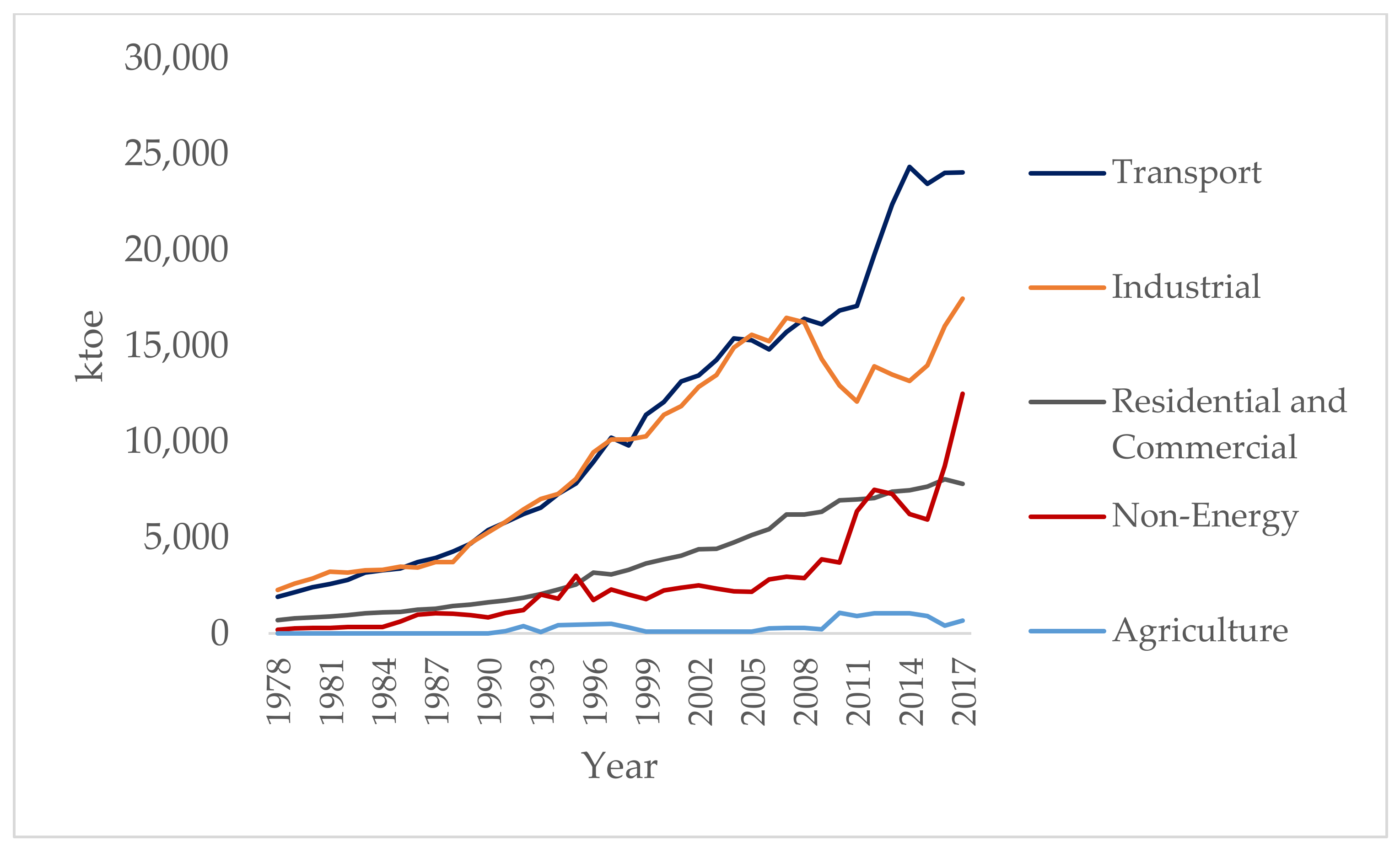
The contribution of the transport sector to the final energy consumption of Malaysia is among the highest across all sectors of energy use. Final energy use in the transport sector has shown to be the most urgent issue to be addressed by the Malaysian government. Since the late 1970s, along with industrial sector use, it has almost the same share until 2008 when a divergent trend began to appear, and the transport sector’s consumption continued to rise exponentially while industrial sector energy demand mellowed (Figure 1). 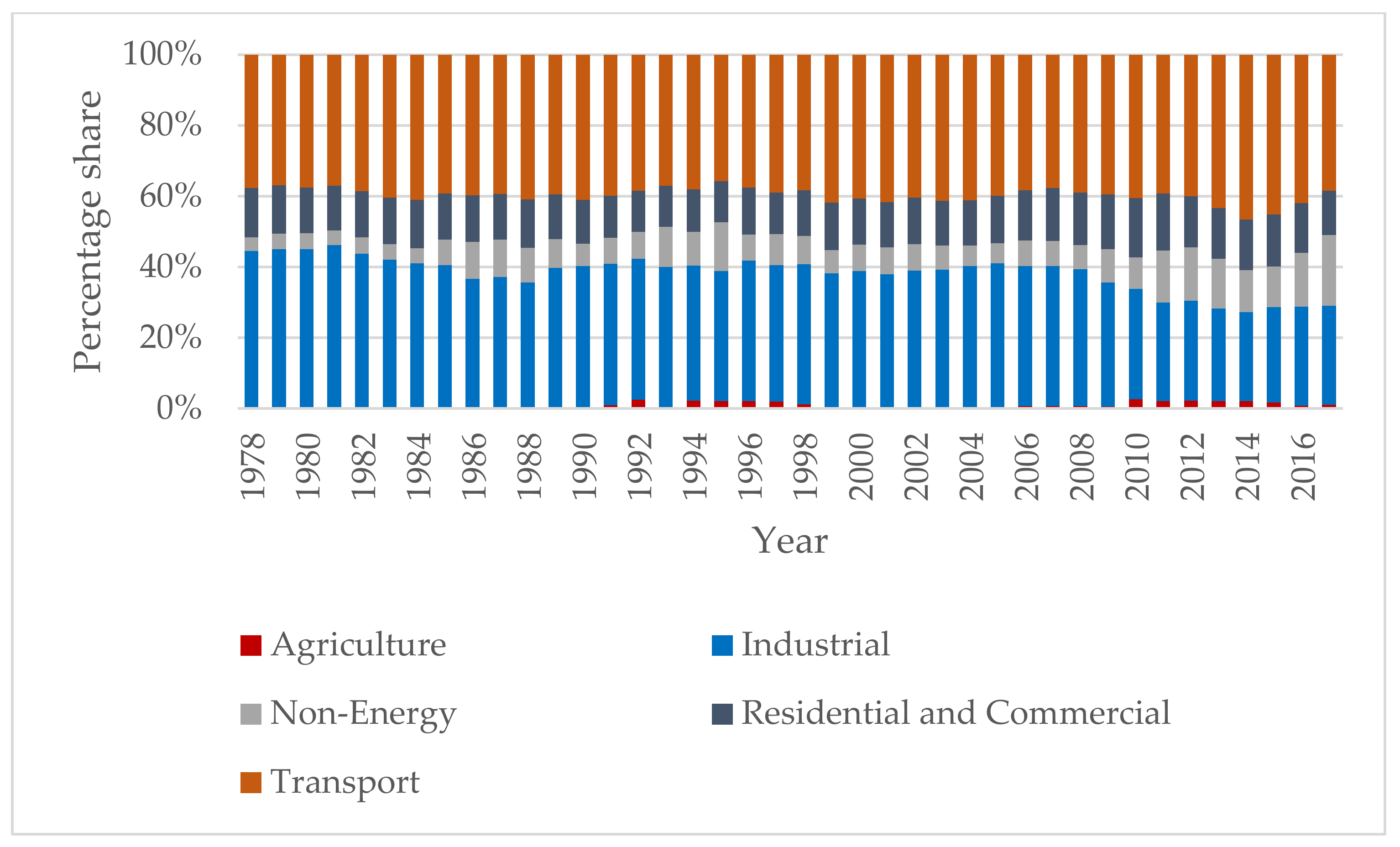In 2014, the share of final energy use by the transport sector breached 46%, the highest in history and was still hovering above 40% in the year 2017 (Figure 2).

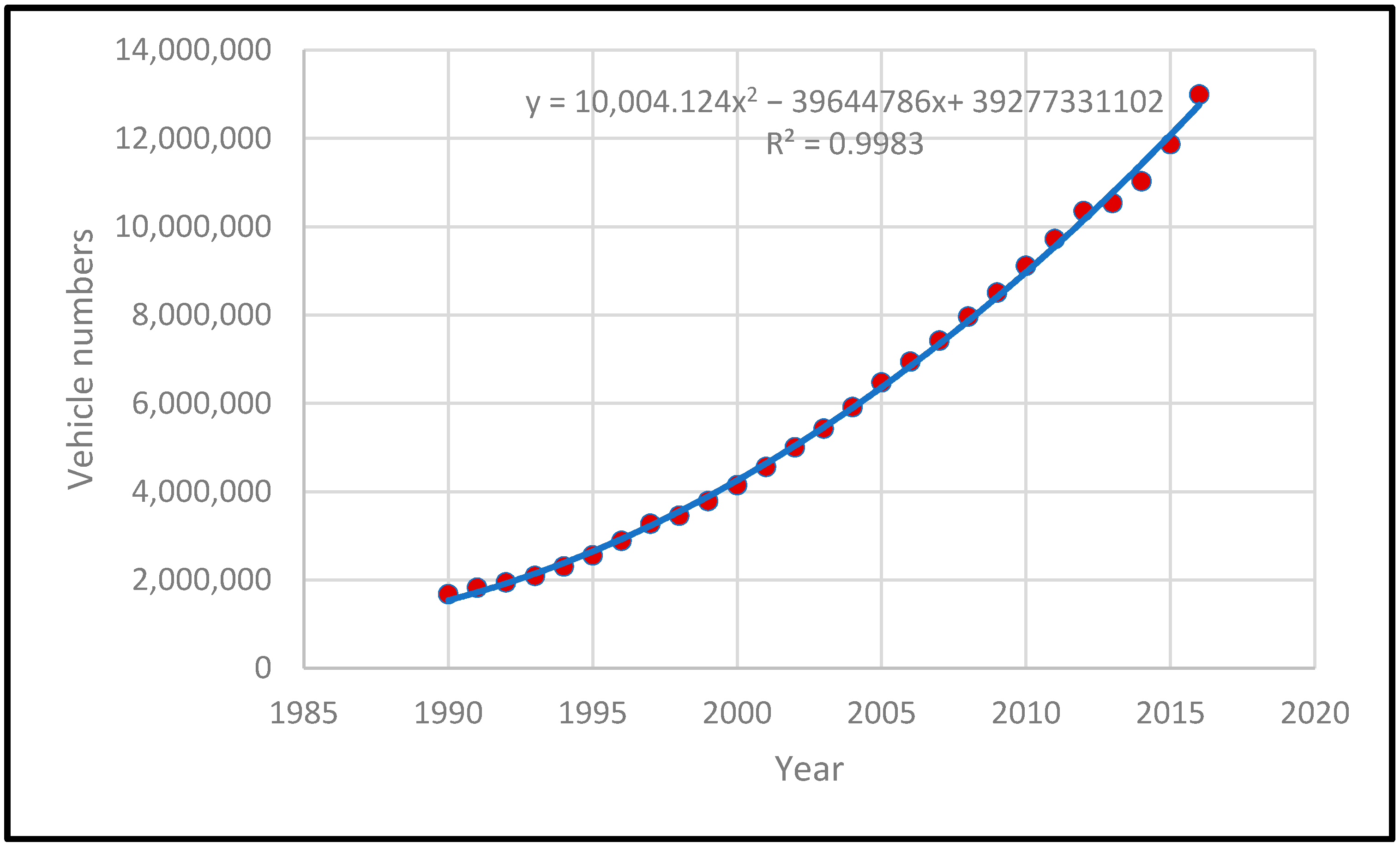
While the transport sector comprises the land, marine and air sector, this analysis focuses on land transport, primarily the use of petrol fuel in the internal combustion engine (ICE) motor vehicles, specifically cars. The increase in the rate of motorisation, including light-duty vehicles (LDV) or cars, has been steady since early the 1990s [3,4]. This focus is due to the enormous growth in car numbers, from around 4 million in 2000 to almost 13 million units in 2016 [5]. In addition, this segment of land transport is the biggest user of energy in the sector. Therefore, addressing energy use by the ever-increasing fleet of cars is imperative to reduce fuel consumption and mitigate its ensuing emissions. In this study, this is achieved by improving the fuel economy of cars.

For this study, we define FE as a measure of how energy efficient a motor vehicle is, commonly understood as the rate of its fuel consumption measured by calculating the amount of fuel used for every unit distance travelled [6]. FE is also driven by essential factors, including powertrain efficiency to convert fuel energy to functional work at the wheels, vehicle weight, speed, aerodynamics, tyres rolling resistance and many more [6]. However, the simple idea of energy use per unit distance moved is the working definition adopted by governments and international organisations worldwide in their reports [7,8,9].

There are many ways to improve the FE situation, and these include FE standards, which is a regulatory measure; fuel labelling, which is an information and awareness measure; innovation in vehicle technology; and fiscal measures [7,10,11]. Some of these have been implemented in some developed economies such as Australia, Canada, the EU and the US, with some early adopters in Asia, including China, India, Japan and South Korea [7,8,12,13]. In the Southeast Asian (SEA) region, Singapore, Vietnam and Thailand had introduced a vehicle fuel economy labelling scheme in 2012, 2014 and 2015, respectively [14], whereas fuel economy labels are voluntary in Indonesia. While no ASEAN member states have mandatory FE standards, fuel consumption or CO₂ emissions policies, Singapore and Thailand have fiscal policies on vehicles based on their emissions [9].

The focus of this study is the benefits of having a Fuel Economy (FE) standard, which improves the fuel economy of these vehicles by a mandatory measure [10,15]. FE standard is a type of regulation that sets a limit to vehicle fuel consumption for new vehicles entering the market when the standard is in place [7,9]. This is done by the introduction of specific regulations by the government, for example, the Corporate Average Fuel Economy Standards (CAFE) in the US [16,17] and the ‘Top Runner’ energy efficiency program in Japan [8,11]. These regulations compel the vehicle manufacturers to meet the FE target set by the regulator by making their vehicles more fuel-efficient, not at the individual vehicle level, due to factors that drive FE described above. However, it is designed as a fleet-wide average to allow for a flexible mix of various models introduced into the market, like the US CAFE [8]. It is a fact that Malaysia has yet to have implemented FE standard measure for its car market. Implementing a FE standard policy for cars in Malaysia is needed to reduce its ever-increasing fuel use and emissions in the transport sector, which depends on the dedication and will of the government to implement this measure. This study analyses and discuss just how much energy can be saved and emissions can be curbed by this measure. Without FE standard policy, there is no push for the automotive industry to introduce new car models into the market with the best fuel-efficient technology. If this is coupled with the fuel price situation, which is subsidised in the form of sales tax exemption, unnecessary fuel use will continue to prevail [18], at the expense of the national fiscal situation, health of the people and the environment. By introducing this policy, Malaysia has the opportunity to address these pressing issues.

2. Methods

For this study, we have adapted the method developed by [19] to investigate the impact of adopting a fuel economy standards policy on passenger vehicles. We employed many of the equations and explain the principles of calculations in the subsequent sections. We have listed the symbols employed in the Nomenclature list. In short, we will first forecast the number of cars and fuel consumption amount using a polynomial curve-fitting method of the latest published data. These are used to determine the average fuel use per unit distance travel (the FE of the car) for each year in the available and forecasted data. There will be a natural improvement of FE, even without the imposition of FE standard due to normal automotive technology advancement. We forecast the natural improvement of FE and the corresponding fuel use as a business-as-usual (BAU) scenario. We then forecast the number of cars affected by the mandatory FE policy (STD). The affected cars will be imposed a mandatory FE number, based on percentage reduction of BAU FE during the first year of implementation. We then calculate the difference of fuel use under BAU and STD scenarios as fuel savings and its avoided emissions. This method is suitable for fuel use analysis at the macro level, where we do not have granular insights into the respective car segment. The flexibility of this method was utilised by [20] in their study to calculate fuel savings. This study includes the added analysis of greenhouse gas emissions mitigation, not previously calculated by [20].

We sourced input data for the model from various government reports, statistics and previous literature. The numbers of privately owned vehicles were sourced from [5,20]. Energy consumption in the form of petrol fuel data was sourced from [1]. We only include vehicles that run on petrol (gasoline) for this study. 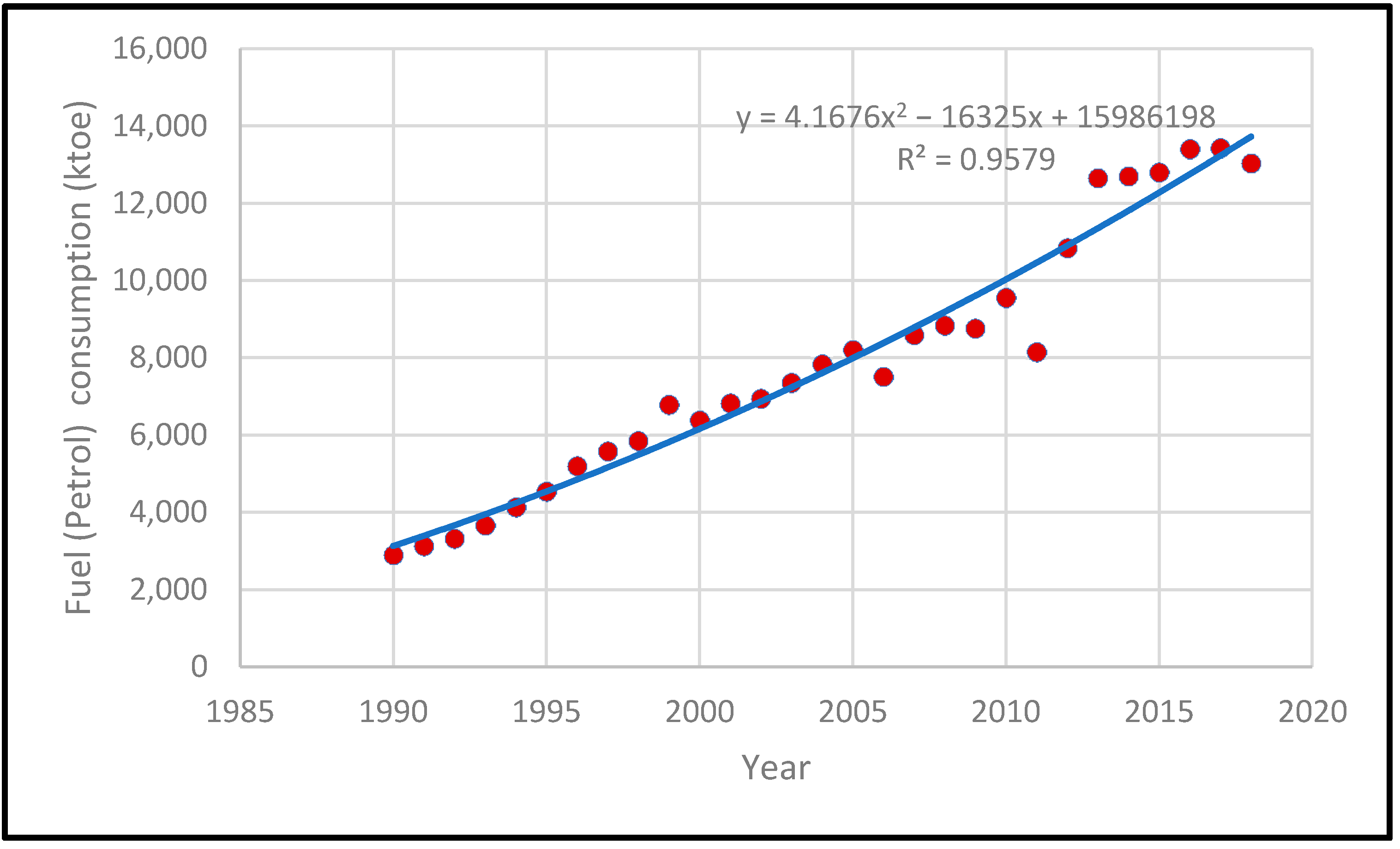The focus on petrol was based on the substantial number of petrol-powered ICE cars (taken to be 89% overall) compared with non-petrol-powered vehicles [21]. The annual petrol fuel consumption (1990–2018) and the corresponding total number of cars (1990 to 2016) are taken from various sources and demonstrated in

Table 1. The annual petrol fuel consumption and number of cars [1,5,20].

Year 1,2,3	Petrol Fuel Consumption (ktoe)	Cars (Units)
1990	2901	1,678,980
1991	3135	1,824,679
1992	3326	1,942,016
1993	3666	2,088,300
1994	4139	2,302,547
1995	4548	2,553,574
1996	5205	2,886,536
1997	5586	3,271,304
1998	5854	3,452,854
1999	6793	3,787,047
2000	6387	4,145,982
2001	6827	4,557,992
2002	6948	5,001,273
2003	7360	5,426,026
2004	7839	5,898,142
2005	8211	6,473,261
2006	7517	6,941,996
2007	8600	7,419,643
2008	8842	7,966,525
2009	8766	8,506,080
2010	9560	9,114,920
2011	8155	9,721,447
2012	10,843	10,354,678
2013	12,656	10,535,575
2014	12,705	11,028,296
2015	12,804	11,871,696
2016	13,411	12,997,839
2017	13,437	-
2018	13,041	-

¹ Vehicle numbers 1990–2008 from [20], ² Vehicle numbers 2009–2016 from [5], ³ Fuel consumption 1990–2018 from [1].

.

2.1. Projection of Petrol Fuel Consumption and Motor Vehicle Numbers

The basis of reduction in petrol fuel consumption and its corresponding emissions realised by the FE standards implementation hinges upon two important factors, namely the annual fuel consumption and motor vehicle numbers. The polynomial regression is instrumental and reliable in projecting future values beyond the presently available data. We define variable x as the number of the year, whereas variable y is the number of cars and petrol fuel consumption as a function of available data x. Polynomial regression enables the best fit line to fit available data points to make future predictions. The following equation represents a polynomial function of order k in x used in this study:

Y = C₀ + C₁ x + C₂ x² + … + C_k x^k

(1)

2.2. Potential Fuel Savings Calculations

2.2.1. Base Year Baseline Fuel Consumption, ${\mathrm{BFC}}_{{\mathrm{Y}}_{\mathrm{B}}}$

The baseline fuel consumption is the current state of affairs, also called the BAU situation. The base year ${\mathrm{Y}}_{\mathrm{B}}$ is taken as the year 2018 as the latest of the real data available. It is easy to determine the baseline fuel consumption for products with standards already implemented, taken as the standard or the rating level. Since Malaysia has no fuel FE standard for cars, we assumed that the baseline fuel consumption for cars is equal to the annual average of fuel consumption of cars. The total fuel consumption (petrol) in litres divided by the numbers of petrol-powered ICE cars in Malaysia, as per the following equation:

$${\mathrm{BFC}}_{{\mathrm{Y}}_{\mathrm{B}}}=\frac{{\mathrm{FC}}_{\mathrm{i}}}{{\mathrm{NV}}_{\mathrm{i}}} \left(\mathrm{L}\right)$$

(2)

2.2.2. Average Annual Fuel Economy Rating, ${\mathrm{FER}}_{\mathrm{i}}$

We calculate the fuel economy of a motor vehicle by averaging the distance travelled by the unit of fuel consumed, typically measured in either miles per gallon (mpg) or kilometres per litres (km/L). The average annual kilometres travelled by car is multiplied by the total number of cars divided by the total fuel consumption in litres. The average fuel economy rating is then:

$${\mathrm{FER}}_{\mathrm{i}}=\mathrm{AM}\times \frac{{\mathrm{NV}}_{\mathrm{i}}}{{\mathrm{FC}}_{\mathrm{i}}} (\mathrm{km}/\mathrm{L})$$

(3)

2.2.3. Annual Fuel Economy Improvement, ${\mathrm{AFI}}_{\mathrm{i}}$

This parameter is the overall percentage improvement of all cars’ fuel consumption on a year-on-year basis. This results from natural technological advancement in automotive technology that enables the cars, overall to travel the same average distance with less fuel. This parameter is represented by the following equation:

$${\mathrm{AFI}}_{\mathrm{i}}=\left[\frac{{\mathrm{FER}}_{\mathrm{i}}-{ \mathrm{FER}}_{\mathrm{i}-1}}{{\mathrm{FER}}_{\mathrm{i}-1}}\right] \times 100 \left(\%\right)$$

(4)

2.2.4. Future Baseline Fuel Consumption, ${\mathrm{BFC}}_{{\mathrm{Y}}_{\mathrm{s}}}$

We define this parameter as the baseline for petrol fuel use by the whole car population in the policy implementation year (Y_s) in a BAU scenario. This parameter is predicted from the projection of the fuel consumption that experiences natural fuel economy improvement over the years. The ${\mathrm{BFC}}_{{\mathrm{Y}}_{\mathrm{B}}}$ is applied a compounding interest function whereby the interest rate is taken as the average of the annual fuel economy improvement (${\mathrm{AFI}}_{\mathrm{avg}}$) (throughout the years of available data), over the number of years from the ${\mathrm{Y}}_{\mathrm{B}}$ and ${\mathrm{Y}}_{\mathrm{s}}$. ${\mathrm{BFC}}_{{\mathrm{Y}}_{\mathrm{s}}}$ is represented by:

$${\mathrm{BFC}}_{{\mathrm{Y}}_{\mathrm{s}}}={\mathrm{BFC}}_{{\mathrm{Y}}_{\mathrm{B}}}\times {\left(1+{ \mathrm{AFI}}_{\mathrm{avg}}\right)}^{\left({\mathrm{Y}}_{\mathrm{s}}-{ \mathrm{Y}}_{\mathrm{B}}\right)} \left(\mathrm{L}\right)$$

(5)

2.2.5. Fuel Consumption under FE Standard Implementation, ${\mathrm{SFC}}_{{\mathrm{Y}}_{\mathrm{S}}}$

The fuel consumption under FE standard implementation is the discounted value of the ${\mathrm{BFC}}_{{\mathrm{Y}}_{\mathrm{s}}}$ of the percentage reduction of fuel use applied under the FE standard. It is the FE improvement from the future baseline fuel consumption, demonstrated as follows:

$${\mathrm{SFC}}_{{\mathrm{Y}}_{\mathrm{S}}}={\mathrm{BFC}}_{{\mathrm{Y}}_{\mathrm{s}}}\times \left(1-{ \mathsf{\eta }}_{\mathrm{s}}\right) \left(\mathrm{L}\right)$$

(6)

2.2.6. Initial Unit Fuel Savings, ${\mathrm{UFS}}_{{\mathrm{Y}}_{\mathrm{S}}}$

Initial unit fuel savings is the difference between the baseline fuel consumption in the first year FE standard is rolled out (BAU, in the absence of FE standard) and the reduced petrol use of the cars under the implementation of the FE standard (applicable to the affected vehicles under the standard). The expression for the initial unit fuel savings is as follows:

$${\mathrm{UFS}}_{{\mathrm{Y}}_{\mathrm{S}}}={\mathrm{BFC}}_{{\mathrm{Y}}_{\mathrm{s}}}-{ \mathrm{SFC}}_{{\mathrm{Y}}_{\mathrm{s}}} \left(\mathrm{L}\right)$$

(7)

2.2.7. Shipment, ${\mathrm{Sh}}_{\mathrm{i}}$

We adapted the concept of ‘shipment’ from [19]. This parameter is a description of the included stock of cars under the FE standard implementation, as not all cars in the first year FE standard is rolled out is included by the policy, namely the previous year’s model of the cars. The number of cars affected by the FE standard is the sum of the difference between the number of cars in the current and the past year (the newly registered cars in the current year), and the replacement stock of the scrapped cars the same year (due to reaching its end-of-life). For example, if the general lifespan L of the vehicles is ten years, then these cars will be scrapped in 10 years time, and the total replacement for these cars will be back in the system in the 11th year. The following expression demonstrates the concept of shipment of the cars:

$${\mathrm{Sh}}_{\mathrm{i}}=\left({\mathrm{NV}}_{\mathrm{i}}-{ \mathrm{NV}}_{\mathrm{i}-1}\right)+{\mathrm{NV}}_{\mathrm{i}-\mathrm{L}} \left(\mathrm{units}\right)$$

(8)

2.2.8. Overall Fuel Economy Improvement, ${\mathrm{TI}}_{{\mathrm{Y}}_{\mathrm{s}}}$

We define the overall fuel economy improvement as a measure of the initial unit fuel savings from the future baseline fuel (in Y_s). The parameter is expressed as:

$${\mathrm{TI}}_{{\mathrm{Y}}_{\mathrm{s}}}=\frac{{\mathrm{UFS}}_{{\mathrm{Y}}_{\mathrm{S}}}}{{\mathrm{BFC}}_{{\mathrm{Y}}_{\mathrm{s}}}} \times 100 \left(\%\right)$$

(9)

2.2.9. Scaling Factor, ${\mathrm{SF}}_{\mathrm{i}}$

The scaling factor is a concept of the natural decrease of fuel consumption of the overall available cars in the country. This parameter is enabled by natural technological advances in the automotive industry, making the cars more fuel-efficient over time, even without the enforcement of an FE standard. Scaling factor reduces the initial unit fuel savings of the cars over the effective span of the policy implementation in a linear manner. In each year after the implementation of the FE standard, this parameter affects the unit fuel savings in that particular year. The scaling factor is expressed as:

$${\mathrm{SF}}_{\mathrm{i}}=1-\left({\mathrm{Y}}_{{\mathrm{Sh}}_{\mathrm{i}}}-{ \mathrm{Y}}_{\mathrm{s}}\right) \frac{{\mathrm{AFI}}_{\mathrm{avg}}}{{\mathrm{TI}}_{{\mathrm{Y}}_{\mathrm{s}}}} \left(\mathrm{dimensionless}\right)$$

(10)

2.2.10. Unit Fuel Savings, ${\mathrm{UFS}}_{\mathrm{i}}$

This parameter is the value of the unit fuel savings for each year after the implementation of FE standard. Due to the natural technological advancement in the automotive industry as described above, this value is adjusted with the scaling factor $S{F}_i$ annually, and expressed as:

$${\mathrm{UFS}}_{\mathrm{i}}={\mathrm{SF}}_{\mathrm{i}}\times { \mathrm{UFS}}_{{\mathrm{Y}}_{\mathrm{S}}} \left(\mathrm{L}\right)$$

(11)

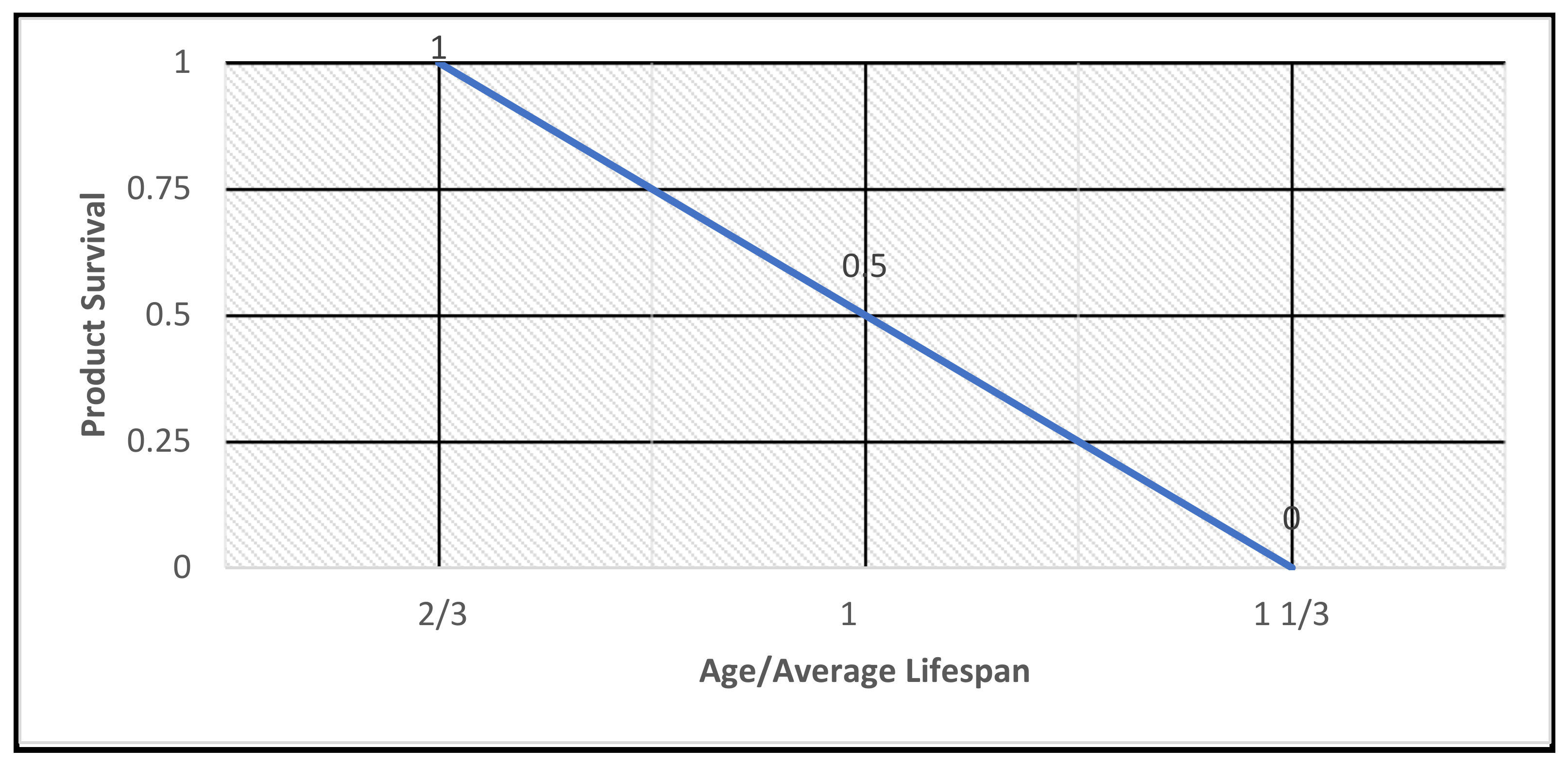
2.2.11. Shipment Survival Factor, ${\mathrm{SSF}}_{\mathrm{i}}$

The ${\mathrm{SSF}}_{\mathrm{i}}$ is a concept of the common survival rate of a product in light of its average lifespan L. The concept is introduced in [19,22]. The ‘shipment’ of the cars will survive 100% up to 2/3 of its lifespan L. If the age of the car’s stock is more than 2/3 of average lifespan L but less than 1 1/3 of the average lifespan L, the survival rate is expressed as [2 − Age × 1.5/(Average Life)]. For the age of over 4/3 of its average lifespan L, 0% of the stock survives. This factor can be graphically demonstrated as per Figure 3.

2.2.12. Affected Stock, ${\mathrm{AS}}_{\mathrm{i}}$

We define the affected stock of cars for the adherence to the FE standards as the shipment of cars in the specific year multiplied by the shipment survival factor, plus the number of cars under the standards in the previous year. Therefore, the expression for the parameter is as follows:

$${\mathrm{AS}}_{\mathrm{i}}=\left({\mathrm{Sh}}_{\mathrm{i}}\times { \mathrm{SSF}}_{\mathrm{i}}\right)+{ \mathrm{AS}}_{\mathrm{i}-1} \left(\mathrm{unit}\right)$$

(12)

2.2.13. Fuel Savings, ${\mathrm{FS}}_{\mathrm{i}}$

The fuel savings are the actual savings of fuel consumed under the FE standard implementation. It is determined by the unit fuel savings and the applicable stock and expressed as:

$${\mathrm{FS}}_{\mathrm{i}}= {{\displaystyle \sum }}_{\mathrm{i}={ \mathrm{Y}}_{\mathrm{s}}}^{\mathrm{T}}\left({\mathrm{AS}}_{\mathrm{i}}\times { \mathrm{UFS}}_{\mathrm{i}}\right) \left(\mathrm{L}\right)$$

(13)

2.3. Potential Emissions Reduction, ER_i

Emissions can potentially be reduced when there is substantial fuel saving resulting from the FE standard implementation. The most common tailpipe emissions of cars include methane (CH₄), carbon monoxide (CO), carbon dioxide (CO₂₎, nitrous oxide (N₂O), nitrogen oxides (NO_X) and sulphur dioxide (SO₂). The tailpipe emissions avoided are calculated from the total fuel savings and the emission factors of the respective gases per unit litre of petrol. The emissions reduction is therefore expressed by:

$${\mathrm{ER}}_{\mathrm{i}}={\mathrm{FS}}_{\mathrm{i}}\times \left({\mathrm{Em}}_{{\mathrm{CH}}_4}+{ \mathrm{Em}}_{\mathrm{CO}}+{ \mathrm{Em}}_{{\mathrm{CO}}_2}+{ \mathrm{Em}}_{{\mathrm{N}}_2\mathrm{O}}+{ \mathrm{Em}}_{{\mathrm{NO}}_{\mathrm{x}}}+{ \mathrm{Em}}_{{\mathrm{SO}}_2}\right) \left(\mathrm{kg}\right)$$

(14)

3. Results and Discussion

Based on the method described, we demonstrate sample calculations and the results obtained in this section.

3.1. Data Analysis

The forecasted fuel consumption for private vehicles was calculated with Equation (1). The polynomial regression method was used on the dataset in Table 1. The mathematical equation for the curve fitted plot is shown below, and the plot is shown in Figure 4.

y = 4.168x² − 16,325x + 15,986,198 R² = 0.9579

(15)

The forecasted number of cars can be predicted using the same polynomial regression method and Equation (1) on the dataset in Table 1. The polynomial expression for the curve fitted plot of vehicle numbers is shown below, and the plot is shown in Figure 5.

y = 10,004.124x² − 39,644,786x + 39,277,331,102 R² = 0.9983

(16)

We tabulated the forecasted petrol fuel consumption of cars and the number of cars in Malaysia from 2010 until 2020 by using the polynomial regression equation in

Table 2. The forecasted number of cars running on petrol and its petrol fuel consumption.

Year	Car Petrol Fuel Consumption (ktoe)	Car Petrol Fuel Consumption (Litres)	Number of Cars
2019	14,222	18,649,416,515	13,285,168
2020	14,730	19,315,158,648	13,963,231
2021	15,246	19,991,830,550	14,659,102
2022	15,770	20,679,432,222	15,372,780
2023	16,303	21,377,963,664	16,104,266
2024	16,844	22,087,424,876	16,853,558
2025	17,394	22,807,815,857	17,620,658
2026	17,951	23,539,136,608	18,405,566
2027	18,517	24,281,387,128	19,208,281
2028	19,092	25,034,567,418	20,028,803
2029	19,674	25,798,677,478	20,867,132
2030	20,265	26,573,717,307	21,723,269
2031	20,865	27,359,686,906	22,597,213
2032	21,473	28,156,586,275	23,488,965
2033	22,089	28,964,415,413	24,398,523
2034	22,713	29,783,174,321	25,325,890
2035	23,346	30,612,862,999	26,271,063

. Since the subsequent fuel economy calculations will be in litres, this study converted the data on energy use published by the Energy Commission in toe (or ton oil equivalent, which is the measure of the energy contained in a metric ton of crude oil) into the appropriate unit of measurement. Therefore, the study adopted the conversion factor whereby 1 ktoe equals the net calorific value of 43.9614 TJ for petrol [1].

3.1.1. Potential Fuel Savings Calculation

The year 2018 was taken as the base year for the baseline fuel consumption calculation. The calculation used Equation (2) and shown below:

$${\mathrm{BFC}}_{2018}=\frac{17,100,410,816}{12,624,912}=1354 \mathrm{L}$$

A total of 17,100,410,816 litres of petrol were consumed in the year 2018. We derived this number from published petroleum products final energy use data for 2018, reported in kilotonnes of oil equivalent (ktoe) unit. We then converted the value to the unit litres by adopting the conversion factor for toe to GJ and GJ to litres of petrol [1,23], whereby one ktoe of energy is equal to 1,311,280.64 L of gasoline (petrol) [23].

There were 12,624,912 cars using petrol fuel in the year 2018. This number represented 89% of the overall motor vehicle numbers for the year. The overall motor vehicle numbers were derived from the polynomial expression in Equation (1). The share of 89% for gasoline (petrol) powered internal combustion engine (ICE) cars (out of the overall total) were adopted from the work of [21]. Therefore, we assumed that petrol ICE cars are 89% of the total number of cars throughout the simulation years for this study.

We used Equations (3) and (4), respectively to calculate the overall fuel economy ratio—FER in km/L—for each year between 1990 and 2018, and the annual fuel economy improvement (AFI), by using the petrol consumption (in litres) and the number of petrol cars, as demonstrated in

Table 3. Fuel Economy Ratio, Annual Fuel Economy Improvement (AFI) and Average AFI.

Year	FER (km/L)	AFI (%)
1990	7.86
1991	7.90	0.57
1992	7.93	0.32
1993	7.73	−2.44
1994	7.55	−2.34
1995	7.62	0.93
1996	7.53	−1.23
1997	7.95	5.60
1998	8.01	0.72
1999	7.57	−5.48
2000	8.81	16.44
2001	9.06	2.85
2002	9.77	7.81
2003	10.01	2.42
2004	10.24	2.29
2005	10.70	4.54
2006	12.54	17.14
2007	11.71	−6.58
2008	12.23	4.43
2009	13.17	7.70
2010	12.94	−1.74
2011	16.18	25.03
2012	12.96	−19.89
2013	11.30	−12.83
2014	11.78	4.27
2015	12.59	6.82
2016	13.16	4.53
2017	13.60	3.38
2018	14.77	8.56
Average		2.64%

. Another critical assumption for this calculation was the average annual distance travelled per car of 20,000 km. We then calculated the average of the AFI (${\mathrm{AFI}}_{\mathrm{avg}}$), which was 2.64% based on each known AFI from the year 1991 to 2018. Consequently, we used the ${\mathrm{AFI}}_{\mathrm{avg}}$ value in Equation (5) to forecast the baseline fuel consumption during the first year of the FE standards roll-out (${\mathrm{BFC}}_{{\mathrm{Y}}_{\mathrm{s}}}$—in the year 2025). For this case, based on known BFC in the year 2018, the baseline fuel consumption in the implementation year of the standard (2025) is shown below:

$${\mathrm{BFC}}_{{\mathrm{Y}}_{\mathrm{s}}}={\mathrm{BFC}}_{2025}={1354 \times (1+2.64\%)}^{(2025-2018)}=1625.12 \mathrm{L}/\mathrm{year}$$

The remaining analysis required some other data and statistics for the basis of assumptions used. There are many improvements needed in the data recording, maintenance and reporting for the transport sector in Malaysia. In lieu of the lack of data, these data estimates were nevertheless adapted from [24,25] and summarised in

Table 4. Input data for calculation of potential fuel savings.

Description	Values
Implementation Year	2025
Average Lifespan	10 years
${\mathrm{BFC}}_{{\mathrm{Y}}_{\mathrm{s}}}$ (${\mathrm{Y}}_{\mathrm{s}}=2025)$	1625.12 L/year
Target FE efficiency improvement	10%
Standards fuel consumption	1333 L/year
Annual mileage	20,000 km/year
Average Annual Fuel Economy Improvement (AFI)	2.64%

.

The potential fuel savings calculation results realised by enforcement of FE standard on cars in Malaysia (beginning year 2025) is outlined in

Table 5. The potential fuel savings calculation results.

Year	Shipment (‘000)	Applicable Stock (‘000)	Scaling Factor	Unit Fuel Savings (L)	Potential Fuel Savings (L)
2025	10,565,809	10,565,809	1.00	162.51	21,090,749,294
2026	11,568,077	22,133,886	0.82	133.95	20,574,304,446
2027	11,982,463	34,116,349	0.65	105.39	20,685,925,377
2028	12,624,912	46,741,261	0.47	76.83	21,443,597,561
2029	13,285,168	60,026,429	0.30	48.26	22,901,509,777
2030	13,963,231	73,989,660	0.12	19.70	25,115,885,234

. As can be seen, the efficacy of the policy lasts for only a few years before the natural improvement of the AFI, due to the advancement of automotive technology, catches up with the target fuel savings of the standards. Based on the previous data, it was assumed that the annual AFI will improve at 2.64% on average, without the FE standard policy in place. Therefore, if the fixed FE standard is not revised to the latest relevant base year, the FE standard’s savings will cease to be relevant a few years after its implementation. As a demonstration of this point, based on Table 5 and Figure 6, the FE standard of 15% reduction based on the year 2025 will be effective for six years, up to the year 2030.

It can be seen in Figure 6 that substantial savings will begin in the first year of the FE standard implementation and continues to increase as more applicable stock gets into the system after the year 2025. After that, however, this effect starts to taper off four years into the FE standard implementation until it ceases to be relevant after the year 2030. This situation happens as the effect of reducing scaling factor kicks in due to the natural increase of the technological advancement in automotive technologies that increases the fuel efficiencies of cars against the FE standard.

The comparison between annual fuel consumption in a BAU situation and fuel consumption under FE standard implementation is shown in Figure 7, whereby STD is the potential fuel consumption at the much-reduced level under the FE standard. The total cumulative savings during the years the FE standard policy is effective is more than 16.2 billion litres of petrol or more than 12,300 ktoe. It is nice to be aware that these savings are based on a minimum of 15% efficiency improvement. With continuous technological improvements, the fuel savings for the future period can be better.

3.1.2. Potential Emissions Mitigation

The fuel savings to be achieved may result in tailpipe emissions reduction, which is beneficial to the global environment. Tailpipe emissions from gasoline (petrol) comprise CH₄, CO, CO₂, N₂O, NO_X and SO₂. The amount of emissions avoided is a function of the emission factors and the amount of petrol saved. We adapted the emission factors from [20,26] in this study. We did some necessary unit conversions as some factors were originally in the units of gallons, and the emission factors are eventually in the form of kg/L or g/L. Table 6 outlines the corresponding emission factors used in this study.

It is essential to understand these from the lens of its respective Global Warming Potential (GWP), in the normalised units of a reference gas, in this case, the CO₂ in the form of carbon dioxide equivalent (CO₂ eq). Each gas has its GWP factor that measures its propensity to the global warming effects, which depends on the time horizon of 100 years. It is interesting to note that depending on the different time horizons adopted, the GWP factor varies. However, the parties to the Conference of the Parties (COP) to the United Nations Framework Convention on Climate Change (UNFCCC) has adopted the 100-year time horizon since the Kyoto Protocol and reaffirmed in the IPCC Second Assessment Report [27] and IPCC Fifth Assessment Report [28]. We outlined the GWP of the respective gases in Table 6. It is worth noting that CO, SO₂ and NO_x are considered indirect greenhouse gases, as compared to CO₂, CH₄ and N₂O, which has direct global warming potential. Therefore, we excluded the effects of CO, SO₂ and NO_x on global warming from this study as indirect greenhouse gases can be highly uncertain, compared with direct GWPs, believed to be highly accurate [29].

Table 6. The emission factor for motor gasoline (petrol) and Global Warming Potential (GWP) of gases.

Type of Emission	Emission Factor 1,2	Emission Factor	GWP 3
CO2	8.78 kg/gal	2.319 kg/L	1
CH4	0.38 g/gal	0.100 g/L	21
N2O	0.08 g/gal	0.021 g/L	310
CO	3.49086 kg/GJ	116.400 g/L	indirect
SO2	0.00228 kg/GJ	0.076 g/L	indirect
NOX	1.36876 kg/GJ	45.630 g/L	indirect

¹ Emission factor for CO₂, CH₄, and N₂O from [26]; ² Emission factor for CO, SO₂, and NO_X from [20]; ³ GWP from [30].

Table 6. The emission factor for motor gasoline (petrol) and Global Warming Potential (GWP) of gases.

Type of Emission	Emission Factor 1,2	Emission Factor	GWP 3
CO2	8.78 kg/gal	2.319 kg/L	1
CH4	0.38 g/gal	0.100 g/L	21
N2O	0.08 g/gal	0.021 g/L	310
CO	3.49086 kg/GJ	116.400 g/L	indirect
SO2	0.00228 kg/GJ	0.076 g/L	indirect
NOX	1.36876 kg/GJ	45.630 g/L	indirect

¹ Emission factor for CO₂, CH₄, and N₂O from [26]; ² Emission factor for CO, SO₂, and NO_X from [20]; ³ GWP from [30].

Table 7. The emissions avoidance calculation results.

Year	CO2 (Ton)	CH4 (kg)	N2O (kg)	CO (kg)	SO2 (kg)	NOX (kg)
2025	3,982,619	172,368	36,288	199,866,548	130,497	78,349,747
2026	6,876,726	297,626	62,658	345,106,464	225,327	135,285,292
2027	8,339,428	360,932	75,986	418,511,748	273,255	164,060,920
2028	8,329,009	360,481	75,891	417,988,891	272,914	163,855,955
2029	6,719,783	290,833	61,228	337,230,320	220,185	132,197,762
2030	3,381,342	146,345	30,809	169,691,653	110,795	66,520,877

¹ Emission factor for CO₂, CH₄, and N₂O from [26]; ² Emission factor for CO, SO₂, and NO_X from [20]; ³ GWP from [30].

shows the result of the emissions avoided throughout FE standard implementation. Consequently, we applied the GWP factor to CO₂, CH₄ and N₂O, and greenhouse gas emission avoidance over the FE standard period, as demonstrated in

Table 8. The greenhouse gas emissions avoidance.

Year	CO2 (Ton)	CH4 (kg CO2 eq)	N2O (kg CO2 eq)
2025	3,982,619	3,619,738	762,050
2026	6,876,726	6,250,145	1,315,820
2027	8,339,428	7,579,571	1,595,699
2028	8,329,009	7,570,102	1,593,706
2029	6,719,783	6,107,502	1,285,790
2030	3,381,342	3,073,247	646,999

.

GHG emissions avoidance can be substantial, especially for CO₂, while CH₄ and N₂O can be negligible relative to the CO₂ scale, as demonstrated by Figure 8. Total CO₂ emissions reduction is 37.6 million tons, while CH₄ and N₂O account for 41,400 tons of CO2 equivalent. Nevertheless, these should count towards the GHG reduction potential as each contribution counts for Malaysia’s commitments to reducing GHG emissions.

4. Conclusions

The analysis in this study for the implementation of the FE standard in the year 2025 is fortunately timed with the commitments of the Malaysian government in reducing its GHG emissions by the year 2030. This study forecasted the stock of cars in the study period and its corresponding fuel savings and emissions mitigation under the FE standard implementation. The key findings that we have found are that, in the period of implementation, fuel savings of 16.2 billion litres of petrol or more than 12,300 ktoe can be achieved, along with the reduction in at least 37.6 million tons CO₂ equivalent GHG emissions. In Malaysia’s official projection to the UNFCCC, under the BAU scenario, the GHG emissions up to the year 2030 (from 2005) is 549,535 Gg CO_{2 eq} (549.535 million Ton CO_{2 eq}), while the mitigation plan scenario is expected to lower this value to 510,205 Gg CO_{2 eq} (510.205 million Ton CO_{2 eq}). The reduction of the overall 39.3 million Ton CO_{2 eq} pledged by Malaysia in its Third National Communication and Second Biennial Update Report to the UNFCCC seems within reach with just this FE standard implementation. These certainly will do well for Malaysia in meeting its commitments to the international community.

The implementation of a FE standard policy for cars in Malaysia is a promising policy to help Malaysia reduce its energy use from the transport sector. This step could be one of the most effective measures, among other FE initiatives [12], nudged positively by the discussion and public discourse of the policy that has happened at various levels within Malaysia and regionally [8,9,31]. However, Malaysia still has a lot to do before the implementation of the FE standard can be realised.

Malaysia has policy documents that outline the intention to have the FE standard implementation timed nicely within the timeframe of this analysis [32,33,34]. Specifically, the Ministry of Transport (MOT) (the ministry in charge of transport policies and regulations) plan to formulate and implement a fuel economy policy between the year 2019 and 2030 [34]. In addition, a further commitment was made by the Ministry of International Trade and Industry (MITI) (the ministry in charge of the development of automotive industry), “pledged to reduce carbon emission by improving fuel economy level in Malaysia by 2025 in line with the ASEAN Fuel Economy Roadmap of 5.3 Lge/100 km” [33]. Both the government automotive and transport policy statements [33,34] for the FE as outlined above indicate that Malaysia is on the right track towards the realisation of the policy.

Despite all these, Malaysia needs to designate a body focusing on the technical aspects and regulatory matters to realise this policy [35]. While various government agencies are related to road transport, prior existing jurisdictions rendered the policy fall in between the cracks, as no specific government agency in Malaysia is responsible for both energy use and transport under its roof. For the technical aspect, one of the actions required involves the driving test cycle suitable for the local situation for measuring the right FE situation. The IEA has outlined the policy pathway and critical actions to implement FE policies, including deciding on the form of standard, target values, introducing a mechanism for increased vehicle weights as part of the policy design process, before implementing and monitoring the progress of the policy implementation [11]. The implementation of FE standard itself should regularly be updated as natural improvements happen over time, rendering the standard obsolete. In addition, conflicting priorities like the encouragement of car ownership as a support to the national automotive industry [3] and curbing energy usage from car use through the implementation of FE standard may impact the competitiveness of the national car industry. This is where Malaysia should resolve its will so that the implementation of the FE standard becomes a reality.

References

1. The Energy Commission. National Energy Balance 2018; The Energy Commission: Putrajaya, Malaysia, 2020. [Google Scholar]
2. The Energy Commission. Final Energy Demand by Sectors; Malaysia Energy Information Hub: Putrajaya, Malaysia, 2019. Available online: https://meih.st.gov.my/statistics?p_auth=SDzwojf5&p_p_id=Eng_Statistic_WAR_STOASPublicPortlet&p_p_lifecycle=1&p_p_state=maximized&p_p_mode=view&p_p_col_id=column-1&p_p_col_pos=1&p_p_col_count=2&_Eng_Statistic_WAR_STOASPublicPortlet_execution=e1s1&_Eng_Sta (accessed on 4 December 2019).
3. Kasipillai, J.; Chan, P. Travel Demand Management: Lessons for Malaysia. J. Public Transp. 2015, 11, 41–55. [Google Scholar] [CrossRef] [Green Version]
4. Ng, W.-S.S. Urban Transportation Mode Choice and Carbon Emissions in Southeast Asia. Transp. Res. Rec. 2018, 2672, 54–67. [Google Scholar] [CrossRef]
5. MAI. Vehicle Registration Statistics for Private Vehicle, Goods Vehicle and Others by Year. 2021. Available online: https://www.data.gov.my/data/ms_MY/dataset/vehicle-registration-statistics-for-private-vehicle-goods-vehicle-and-others (accessed on 15 May 2021).
6. Cleveland, C.J.; Morris, C. Dictionary of Energy, 2nd ed.; Morris, C., Ed.; Elsevier: Boston, MA, USA, 2015; pp. 217–246. [Google Scholar]
7. IEA. Fuel Economy of Road Vehicles; IEA: Paris, France, 2011. [Google Scholar]
8. GFEI. Improving Vehicle Fuel Economy in the ASEAN Region; GFEI: London, UK, 2010. [Google Scholar]
9. ASEAN Secretariat. ASEAN Fuel Economy Roadmap for the Transport Sector 2018–2025: With Focus on Light-Duty Vehicles; ASEAN Secretariat: Jakarta, Indonesia, 2019. [Google Scholar]
10. Atabani, A.; Badruddin, I.A.; Mekhilef, S.; Silitonga, A. A review on global fuel economy standards, labels and technologies in the transportation sector. Renew. Sustain. Energy Rev. 2011, 15, 4586–4610. [Google Scholar] [CrossRef]
11. IEA. Improving the Fuel Economy of Road Vehicles, a Policy Packace; IEA: Paris, France, 2012. [Google Scholar]
12. Lipu, M.S.H.; Hannan, M.A.; Karim, T.F.; Hussain, A.; Saad, M.H.M.; Ayob, A.; Miah, M.S.; Mahlia, T.M.I. Intelligent algorithms and control strategies for battery management system in electric vehicles: Progress, challenges and future outlook. J. Clean. Prod. 2021, 292, 126044. [Google Scholar] [CrossRef]
13. Clerides, S.; Zachariadis, T. The effect of standards and fuel prices on automobile fuel economy: An international analysis. Energy Econ. 2008, 30, 2657–2672. [Google Scholar] [CrossRef]
14. Yang, Z. Overview of global fuel economy policies. In Proceedings of the 2018 AP CAP Joint Forum and Clean Air Week Theme: Solutions Landscape for Clean Air, Bangkok, Thailand, 19–23 March 2018. [Google Scholar]
15. Mallick, P. Materials, Design and Manufacturing for Lightweight Vehicles, 2nd ed.; Mallick, P., Ed.; Woodhead Publishing: Cambridge, UK, 2020. [Google Scholar]
16. Crandall, R.W. Policy Watch: Corporate Average Fuel Economy Standards. J. Econ. Perspect. 1992, 6, 171–180. [Google Scholar] [CrossRef] [Green Version]
17. Portney, P.R.; Parry, I.W.; Gruenspecht, H.K.; Harrington, W. Policy Watch: The Economics of Fuel Economy Standards. J. Econ. Perspect. 2003, 17, 203–217. [Google Scholar] [CrossRef]
18. Ying, L.S.; Harun, M. Fuel subsidy abolition and performance of the sectors in Malaysia: A computable general equilibrium approach. Malays. J. Econ. Stud. 2019, 56, 303–326. [Google Scholar]
19. Mahlia, T.; Masjuki, H.; Choudhury, I. Theory of energy efficiency standards and labels. Energy Convers. Manag. 2002, 43, 743–761. [Google Scholar] [CrossRef]
20. Aizura, A.B.; Mahlia, T.M.I.; Masjuki, H.H. Potential fuel savings and emissions reduction from fuel economy standards implementation for motor-vehicles. Clean Technol. Environ. Policy 2009, 12, 255–263. [Google Scholar] [CrossRef]
21. Ishak, A. Vehicle Inspection in Malaysia. In Proceedings of the Regional Workshop on Vehicle Inspection and Maintenance Policy in Asia, Bangkok, Thailand, 10–12 December 2001. [Google Scholar]
22. Sanchez, M.; Koomey, J.; Moezzi, M.; Meier, A.; Huber, W. Miscellaneous Electricity Use in the US Residential Sector; Lawrence Berkeley National Laboratory: Berkeley, CA, USA, 1998. [Google Scholar]
23. US Energy Infomation Administration. Units and Calculators Explained—Energy Conversion Calculators. 2020. Available online: https://www.eia.gov/energyexplained/units-and-calculators/energy-conversion-calculators.php (accessed on 4 February 2021).
24. Azman, Z.; Radin, D.; Ahmad, R.; Ramdzani, A.; Chung, I. The estimation of carbon dioxide (CO2) emissions from the transport sector in Malaysia (2000–2020). In Proceedings of the 9th AIM International Workshop, National Institute for Environmental Studies, Tsukuba, Japan, 12–13 March 2004. [Google Scholar]
25. Masjuki, H.H.; Karim, M.; Mahlia, T. Energy Use in the Transportation Sector of Malaysia; University of Malaya: Kuala Lumpur, Malaysia, 2004. [Google Scholar]
26. US Environmental Protection Agency. Emission Factors for Greenhouse Gas Inventories. 2014. Available online: https://www.epa.gov/sites/production/files/2015-07/documents/emission-factors_2014.pdf (accessed on 6 May 2021).
27. IPCC. Global Warming of 1.5 °C. An IPCC Special Report; IPCC: Geneva, Switzerland, 2018. [Google Scholar]
28. Myhre, G.; Stocker, T.F.; Qin, D.; Plattner, G.-K.; Tignor, M.M.B.; Allen, S.K.; Boschung, J.; Nauels, A.; Xia, Y.; Bex, V.; et al. Anthropogenic and Natural Radiative Forcing. In Climate Change 2013: The Physical Science Basis. Contribution of Working Group I to the Fifth Assessment Report of the Intergovernmental Panel on Climate Change; IPCC: Geneva, Switzerland, 2013. [Google Scholar]
29. IPCC. Climate Change 2001: The Scientific Basis. Contribution of Working Group I to the Third Assessment Report of the Intergovernmental Panel on Climate Change; IPCC: Geneva, Switzerland, 2001. [Google Scholar]
30. UNFCC. Global Warming Potentials (IPCC Second Assessment Report). 2021. Available online: https://unfccc.int/process/transparency-and-reporting/greenhouse-gas-data/greenhouse-gas-data-unfccc/global-warming-potentials (accessed on 6 May 2021).
31. Briggs, H.G.; Leong, H.K. ASEAN-German Technical Cooperation|Energy Efficiency and Climate Change Mitigation in the Land Transport Sector Malaysia Stocktaking Report on Sustainable Transport and Climate Change Data, Policy, and Monitoring; GIZ: Kuala Lumpur, Malaysia, 2016. [Google Scholar]
32. EPU. Final Report on Demand Side Management (DSM) Preliminary Study; EPU: Putrajaya, Malaysia, 2017. [Google Scholar]
33. Ministry of International Trade and Industry (MITI). National Automotive Policy 2020; Ministry of International Trade and Industry: Kuala Lumpur, Malaysia, 2020. [Google Scholar]
34. Ministry of Transport Malaysia. National Transport Policy 2019–2030; Ministry of Transport Malaysia: Putrajaya, Malaysia, 2019. [Google Scholar]
35. Indati Mustapa, S.; Ali Bekhet, H. International Journal of Energy Economics and Policy Investigating Factors Affecting CO2 Emissions in Malaysian Road Transport Sector. Int. J. Energy Econ. Policy 2015, 5, 1073–1083. [Google Scholar]
Figure 1. Final energy demand by sectors (ktoe), 1978–2017 [1].
Sustainability 13 07348 g001
Figure 2. The percentage share of final energy demand by sectors, 1978–2017 [2].
Sustainability 13 07348 g002
Figure 3. The relationship between the Age/Average lifespan of a product with Product Survival.
Sustainability 13 07348 g003
Figure 4. The prediction of petrol fuel consumption for cars with polynomial regression.
Sustainability 13 07348 g004
Figure 5. The prediction of the number of cars using polynomial regression.
Sustainability 13 07348 g005
Figure 6. The prediction of annual fuel savings for cars.
Sustainability 13 07348 g006
Figure 7. The prediction of annual fuel savings for cars.
Sustainability 13 07348 g007
Figure 8. The greenhouse gas emissions avoidance under the FE standard implementation.
Sustainability 13 07348 g008