Stacking Ensemble Tree Models to Predict Energy Performance in Residential Buildings

Abstract

In this research, a new machine-learning approach was proposed to evaluate the effects of eight input parameters (surface area, relative compactness, wall area, overall height, roof area, orientation, glazing area distribution, and glazing area) on two output parameters, namely, heating load (HL) and cooling load (CL), of the residential buildings. The association strength of each input parameter with each output was systematically investigated using a variety of basic statistical analysis tools to identify the most effective and important input variables. Then, different combinations of data were designed using the intelligent systems, and the best combination was selected, which included the most optimal input data for the development of stacking models. After that, various machine learning models, i.e., XGBoost, random forest, classification and regression tree, and M5 tree model, were applied and developed to predict HL and CL values of the energy performance of buildings. The mentioned techniques were also used as base techniques in the forms of stacking models. As a result, the XGboost-based model achieved a higher accuracy level (HL: coefficient of determination, R² = 0.998; CL: R² = 0.971) with a lower system error (HL: root mean square error, RMSE = 0.461; CL: RMSE = 1.607) than the other developed models in predicting both HL and CL values. Using new stacking-based techniques, this research was able to provide alternative solutions for predicting HL and CL parameters with appropriate accuracy and runtime.

1. Introduction

In recent years, the literature has consisted of many studies carried out into the energy performance of buildings (EPB). Such popularity is because many concerns have been raised regarding energy wastage and the adverse effects of this phenomenon on the natural environment [1,2]. The European Directive 2002/91/EC has determined specific requirements related to energy efficiency to be followed by all buildings constructed in the scope of this continent [2]. As suggested by many studies released across the world during the past decades, energy consumption in the building sector has experienced a steady increase [3,4]. More specifically, most of the energy consumed in this sector is used for heating, ventilation, and air conditioning (HVAC) of the buildings [5]. These three items regulate the indoor climate of buildings [6]. For that reason, an effective way to decline the demands for extra energy supply is to design buildings of higher energy efficiency and enhance the tools required for conserving energy in buildings. To this end, there is a need for calculating two significant items, i.e., cooling load (CL) and heating load (HL), to decide about their equipment specifications, which are essential for keeping indoor air conditions comfortable [5]. Accurate information regarding the building features (e.g., activity and occupancy levels), the climate, and the type of building (industrial/residential) is required. Currently, the literature comprises some extensively used tools for simulating the energy consumption of buildings. They can be applied to analyzing or predicting the building energy consumption, thereby efficiently facilitating energy-building operations. Real-life practice has generally confirmed the high capacity of simulation models in offering an accurate reflection of actual measurements [7]. In many fields of study, simulation tools are of high importance. This is because they help researchers do their experiments with parameters that are infeasible or less feasible in practice [8]. For instance, concerning building energy design, these tools provide a proper environment for comparing similar buildings by modifying only a single parameter among an available range of possible values. To compare the existing building simulation tools in more detail, several references can be found [7,9]. One may achieve dependable solutions with the use of some advanced building energy simulation software to predict the effects of different building design alternatives, though much time and expertise is needed in a specific program. In addition, different building simulation software packages may offer varying levels of accuracy in their results [7].

Numerous studies have preferred to make use of soft computing (SC) and machine learning (ML) tools to examine the impacts of different parameters of building on some variables since this requires much less expertise and time in cases where a database is available containing the required ranges of variables [1,10,11,12,13,14,15,16,17,18]. Using statistical and ML tools in the EPB domain, one can use the benefits of some distinctive advantages provided by refined expertise from other disciplines. With these techniques, especially when a particular model has been sufficiently trained, reliable results could be obtained rapidly by varying some building design parameters. Furthermore, the mentioned techniques/analyses can enhance our understanding by offering quantitative expressions of different effective parameters that the building researchers/designers might need to know. As a result of the above-noted advantages, many researchers have become interested in integrating SC and ML models for solving engineering and science problems [19,20,21,22,23,24,25,26,27,28,29,30,31,32,33,34,35,36,37,38,39,40,41,42,43,44,45,46,47,48,49,50,51,52,53,54,55,56,57,58,59,60,61,62,63,64,65,66,67,68,69,70]. In the context of EPB, different quantities of interest can be well predicted using a variety of SC and ML techniques, e.g., decision trees [1], support vector machines [10,71], polynomial regression [11], and artificial neural networks (ANNs) [72,73]. The literature consists of many studies that have applied SC and ML tools to the prediction of CL and HL. Polynomial regression was utilized by Catalina et al. [11] for forecasting the building heating demand during one month. The parameters of the building shape, the window-to-floor area ratio, the envelope U-value, climate, and the time constant of the building were set as input variables. In another study, Wan et al. [74] investigated the office buildings in China regarding the effects of climate change on CL and HL. Li et al. [71] attempted to predict the hourly building CL based on environmental parameters. Their results revealed that CL and HL are affected by different variables like climate [74], relative compactness (RC) [75], orientation, surface area, wall area, roof area [75,76], and glazing [75]. According to engineers and designers, these variables were examined since they significantly correlated with energy performance, especially with CL and HL. Schiavon et al. [76] examined the impacts of structure type, raised floor, window-to-wall ratio, and the presence of carpet on determining CL for various regions. Their results showed the high significance of two parameters, i.e., the orientation of the building and the presence of carpet, in this regard.

The challenge is that numerous researchers working in EPB have made inflexible assumptions considering merely the classical least squares regression and linear correlations methods. The techniques mentioned above have been found inapplicable to numerous complex problems where normality moulds do not hold. Some other researchers have employed complex SC and ML applications without any success in thoroughly scrutinizing the accessible data (e.g., to identify the critical parameters to a particular problem). Therefore, they have also failed to provide meaningful information that can be well derived using statistical tools. The present paper determines the output variables (i.e., CL and HL of residential buildings) by examining the impacts of eight inputs, including overall height, RC, wall area, surface area, roof area, building orientation, glazing area, and glazing area distribution. In most of the papers published in the EPB area, these variables have been taken into account recurrently to explore the energy-related topics in buildings. The current research explores the data, meticulously analyzes available statistics to gain insight into the essential behavior of model inputs/output, and applies ML tools. In this research, four stacking tree models are developed to predict two HL and CL parameters. The obtained results will then be analyzed and discussed for the purpose of obtaining a powerful ML technique.

2. Research Significance

The accomplishment of sustainable development goals (SDGs) in the energy sector as introduced by Agenda 2030 is a critical issue in many countries [77]. Energy is fundamental to nearly every significant opportunity that humanity confronts today, including health, adaptation to climate change, sustainable cities, and transport [77]. Moreover, according to United Nations [77], energy is the dominant contributor to climate change, accounting for around 60% of total global greenhouse gas emissions. Therefore, energy-saving and designing buildings of higher energy efficiency seems to be a robust remedial response for achieving SDGs.

Energy-saving issues are directly related to socio-economic development and SDGs (Goal 7) as introduced by Agenda 2030 [77]. Goal 7 involves ensuring affordable, reliable, sustainable, and modern energy [77]. Since energy is crucial for achieving many of the SDGs, the significance of this study lies in the development of an efficient tool for calculating two critical items required for proposing energy-saving measures in buildings.

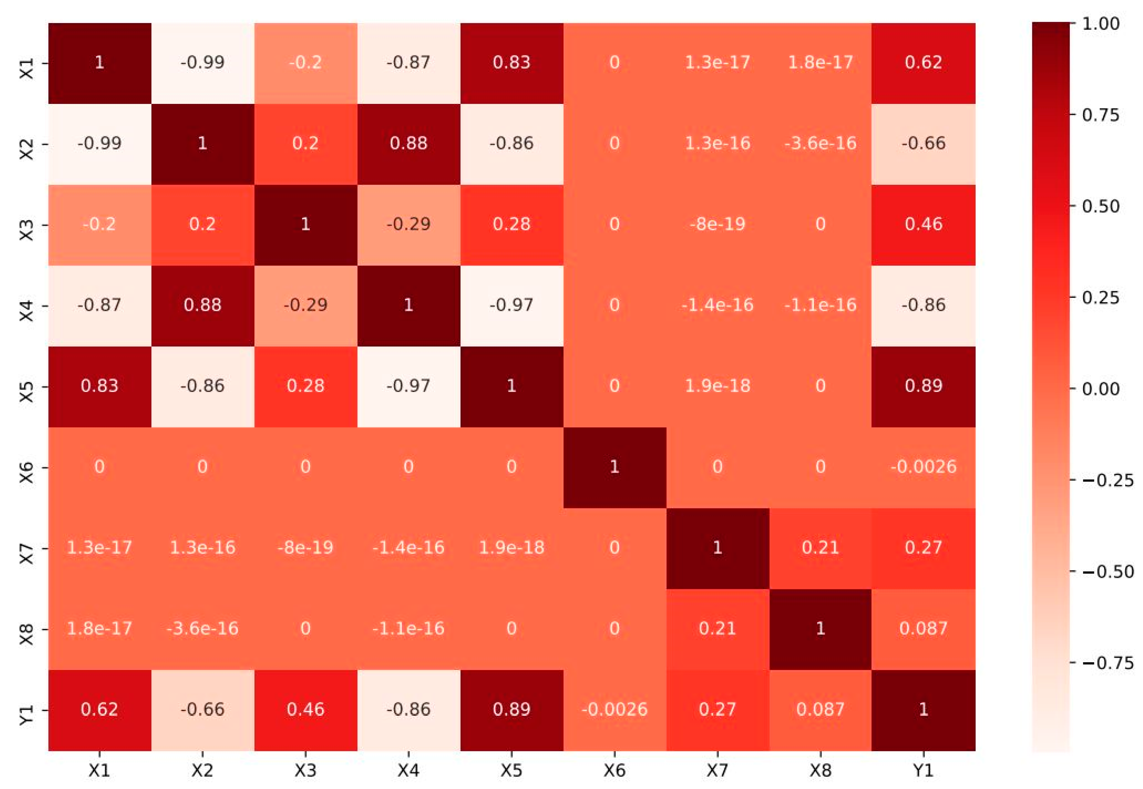
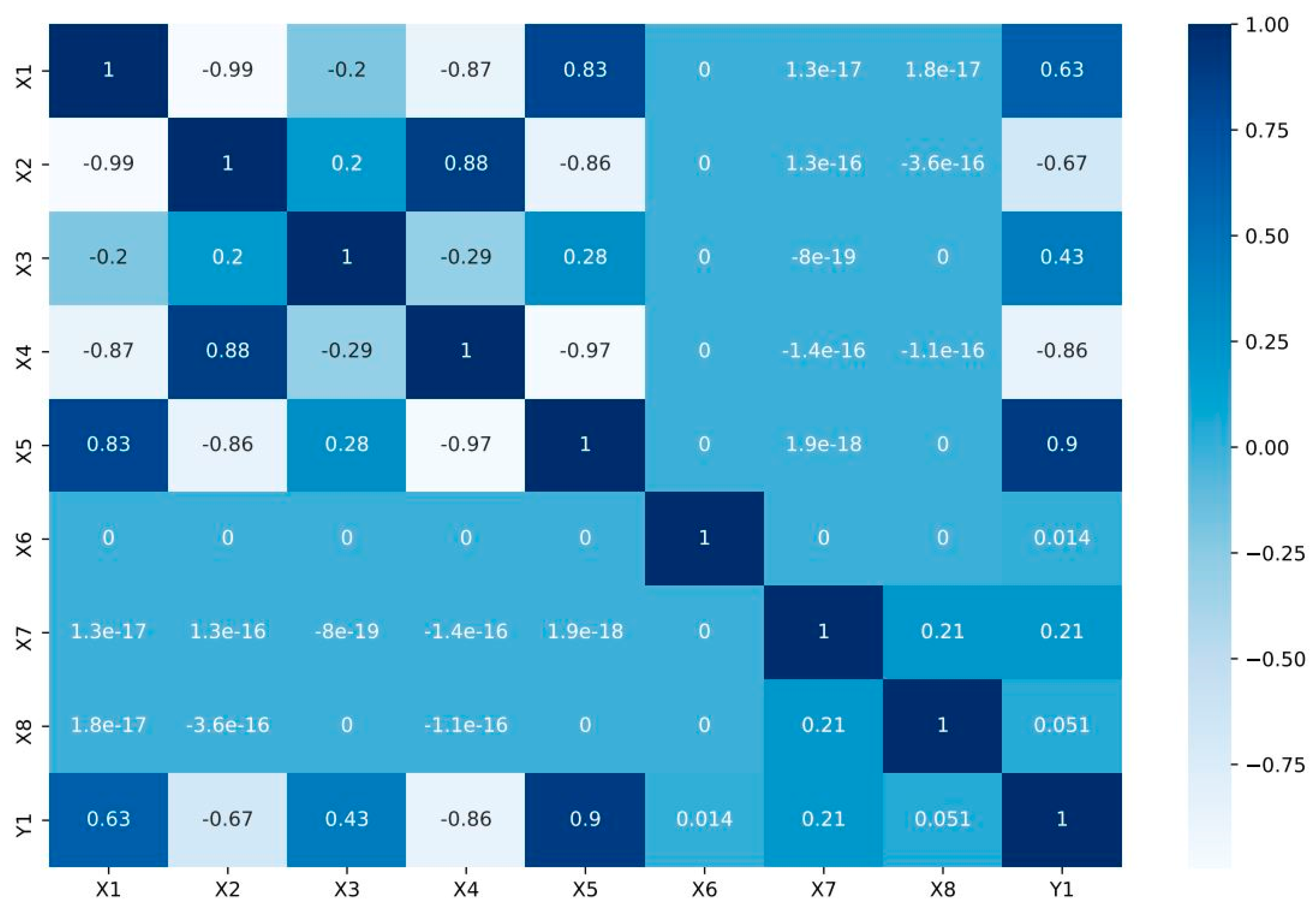
3. Energy Data of Building

An elementary cube (3.5 m × 3.5 m × 3.5 m) was applied to produce 12 building forms, each of which comprised 18 elements (elementary cubes). Ecotect was used to generate the simulated buildings required for this study. All the simulated buildings have similar materials and similar volumes (771.75 m³); however, they differ in their surface areas and dimensions. They were built using modern and extensively used materials used by the building industry, with minimized U-value. Several building specifications were utilized (the associated U-values are noted in parentheses): floors (0.860), walls (1.780), windows (2.260), and roofs (0.500) [74]. In the simulations performed in this study, the assumption was that the buildings are of a residential type and located in Athens, Greece, occupied by seven persons with sedentary activities (70 W). Then, the interior design was planned and considered as follows: clothing: lighting level: 300 Lux, 0.6 clo, airspeed: 0.30 m/s, and humidity: 60%. The internal advances were fixed at sensible (5) and latent (2 W/m²). In this situation, a value of 0.5 was set as the infiltration rate for air change rate with wind sensitivity 0.25 air changer per hour. In the case of thermal conditions, this study implemented a 95% efficiency mixed mode as follows: thermostat range 19–24 °C, with operations on weekends for 10–20 h and 15–20 h on weekdays. Regarding glazing areas/zones, three different kinds were utilized in the simulation, which are articulated as percentages i.e., 10%, 25%, and 40% of the floor area. In addition, for every glazing zone, five distribution scenarios were considered and simulated. For more details, the main research [74] can be considered and reviewed.

Moreover, samples without any glazing areas were achieved as well. At the final step, all forms were rotated in a way to face the four cardinal points. As a result, with taking into consideration 12 building forms and three different glazing areas with five distributions of each glazing area, for four orientations, in total 12 × 3 × 5 × 4 = 720 building samples were considered and obtained. Additionally, 12 building forms were considered for the four orientations with no glazing. Thus, the present paper investigated 12 × 3 × 5 × 4 + 12 × 4 = 768 simulated buildings in total, each of which can be categorized by eight variables (to be well conformed to the standard mathematical notation, to facilitate the analyses required in this study, these building parameters will be named input variables denoted by X) that are to be explored further in the present study. Moreover, in the case of all 768 buildings, CL and HL (which are the output variables and hereafter denoted by y) were recorded. The input/output parameters are summarized in

Table 1. The statistical information of parameters including eight inputs and two outputs.

Parameter	Symbol	Unit	Minimum	Average	Maximum	Variance
Relative compactness	X1	-	0.62	0.76	0.98	0.01
Surface area	X2	m2	514.50	671.71	808.50	7759.16
Wall area	X3	m2	245	318.50	416.50	1903.27
Roof area	X4	m2	110.25	176.60	220.50	2039.96
Overall height	X5	m	3.50	5.25	7	3.07
Orientation	X6	-	2	3.50	5	1.25
Glazing area	X7	m2	0	0.23	0.4	0.02
Glazing area distribution	X8	-	0	2.81	5	2.41
Heating load	Y1	KWh/m2	6.01	22.31	43.1	101.81
Cooling load	Y2	KWh/m2	10.9	24.59	48.03	90.50

, introducing the mathematical representations of the variables and the number of possible values. Many researchers have attempted to simulate energy aspects of buildings, although no one can assure that the simulation results flawlessly show the actual data in the real world (here CL and HL) [74].

4. Methodology

Artificial intelligence, SC, and ML models have been used as alternative solutions to various problems [21,22,31,78,79,80,81,82,83,84,85,86,87]. One of the new structures known as tree structure has recently been developed in various forms. The tree model is applied in numerous modelling fields of hydrology and meteorology. While model trees are able to obtain data-based forecasts by strict guidelines, their efficiency indeed needs to be improved. Bagging or upgrading ensemble strategies are two well-known approaches [88]. Accordingly, there are some reports about using classification and regression tree (CART) or M5 to predict the problem of HL and CL values in the literature. Furthermore, perhaps just a few studies have concentrated on applying several model trees’ stacked ensemble to the breakup timing of EPB. As a result, various sorts of tree models got stacked to combine the benefits of each model in a layered framework.

4.1. Stacking Structure

Several sorts of model trees have been utilized as ensemble models and core models (educators) in a stacking ensemble tree model (SETM) for HL and CL parameters (Figure 1). CART, random forest (RF), M5, and XGboost are put to the test as core models and as ensemble models in the current study. As a foundational ensemble model, the simple average technique (SAM) is used for the modeling of this study. The CART, RF, M5, and XGboost models are briefly described in the following sub-sections, along with the most significant methods for developing the base and ensemble (mixing) models.

4.2. CART

The current work uses CART, first developed by Breiman et al. [89], to estimate the breakup dates of the river ice. The applied CART structure in the study is a regression model with forecasted dependent variable for every leaf node by the sequence of branching nodes as independent variable division criteria [46,90,91,92]. According to the training data set, a binary recursive partitioning procedure is employed to get the best structure. The separation of the database into two subsets is done in an iterative procedure until the prediction total residual sum square (TRSS) values are achieved for all the subsets of the minimum threshold. After every node has been divided, it is compared to each independent variable at all conceivable values, and the split utilization determined by the TRSS improvement gained by dividing that node is smaller than a predetermined threshold or the minimum limit inside that node that is met. The values of independent variables that are newly created in the testing data set are applied to calculate the subnode, into which a sample enters once the CART structure is established according to the training data set. As a consequence, the sample launches into a leaf node sequentially. The forecasted value of the sample’s dependent variable is the mean dependent variable at the leaf node in the training set. CART offers a number of benefits, the most notable of which are: (1) no predefined status of the correlation, (2) no hypothesis about the variable distribution, (3) influential exploration of all potential splits with all independent variables, and (4) simple-to-understand underlying logic. The statistical information and MATLAB Machine Learning Toolbox are used to implement CART in this work.

4.3. M5 Tree Model

The M5 tree model is utilized when the leaf nodes’ differences are not set in CART [93,94]. At each leaf, a regression tree is integrated by M5 with potential linear regression models. Because the decision structure is apparent and the models can characterize the potential difference in every leaf with fewer variables, the resulting tree model has a clear structure with increased fitting capabilities. The M5 tree may be thought of as a piecewise linear model. Keep in mind that setting a regression tree is similar to setting a model of M5 tree. The original tree is built via a recursive splitting technique to reduce the mistake rate. A splitting criterion consists of a specific node from the training data that is obtained through a standard deviation. The splitting operation is terminated when samples’ output difference is lower than the standard deviation of the basic sample. In other words, when their standard deviation is less than 5% of the standard, the basic sample set. Similarly, the division process is terminated when the samples inside a subset falls below a specified threshold. Following that, sonelinear regression models are built in the terminating (leaf) nodes for each sample. The cut back procedure is then conducted to the newly generated tree in order to overcome over-fitting by combining certain lower sub-trees into a single node. Each leaf of the pruned tree is subjected to a smoothing technique in the final phase to remunerate the strong disruptions between surrounding linear models. The new sample prediction is made in two phases using the resultant MT: (1) the new sample is let go of a specific leaf depending on the inputs using the tree’s splitting criteria, and (2) the expert model’s output at the associated leaf is used as one for the new sample. M5 is used in this study with the aid of the MATLAB toolbox created by Jekabsons [95].

4.4. RF

Breiman [96] presented RF as an enhanced version of tree Bagging [97], which merges the random subspace technique and bagging method. The bootstrap approach with simple and feature sampling is used to create the original data subsets. The best split in each decision tree is determined through finding the candidate features’ random-based subset according to a given criterion (i.e., Gini impurity). The voting technique is used to decide the last estimation once the decision trees have been created. Such methods are entirely suitable to the related classification issue in finance-related disciplines because RF does not need for assuming a previous distribution [98] and since the deployment method is simple.

4.5. Extreme Gradient Boosting

Chen and Guestrin [99] created extreme gradient boosting (XGBoost), which is an effective tree-based ensemble learning algorithm. Many academics in the field of data science regard it as a powerful tool. XGBoost is based on the gradient boosting architecture [100], and its objective function is computed as follows:

$$Obj \left(\theta \right)={\displaystyle \sum }_{i=1}^{n}L(y_i, \widehat{y_i})+{\displaystyle \sum }_{k=1}^k\mathsf{\Omega }(f_k)$$

(1)

in which the first portion reflects the model’s training loss (logistic or squared loss) and the second part reflects the total complexity the trees. The kth complexity of the tree is able to be obtained through $\mathsf{\Omega } \left(f\right)=\gamma T+\frac{1}{2}\lambda {\left|\right|w\left|\right|}^2$, in which γ shows the parameter of complexity, T indicates the leaf nodes quantity, λ represents the constant coefficient, and ${\left|\right|w\left|\right|}^2$ demonstrates the l2-norm of the weight of the leaf.

Moreover, the primary goal function can be articulated as shown below following the Taylor expansion:

$$\begin{array}{l}Ob{j}^{\left(t\right)}\approx {\displaystyle {\displaystyle \sum }_{i=1}^n}[L(y_i, \widehat{y_i})+g_i{f}_{i\left(x_i\right)}+\frac{1}{2}{h}_i{f}_i{}^2\left(x_i\right)]+\mathsf{\Omega }\left(f_i\right)\\ ={\displaystyle {\displaystyle \sum }_{i=1}^n}[g_i{w}_q\left(x_i\right)+\frac{1}{2}{h}_i{w}_q{}^2\left(x_i\right)]+\gamma T+\frac{1}{2}{\displaystyle {\displaystyle \sum }_{j=1}^T}{w}_j{}^2\\ ={\displaystyle {\displaystyle \sum }_{i=1}^T}\left[\left({\displaystyle {\displaystyle \sum }_{i=I_j}}{g}_i\right)w_j+\frac{1}{2}\left({\displaystyle {\displaystyle \sum }_{i=I_j}}{h}_i+\lambda \right)w_j{}^2\right]+\gamma T\\ ={\displaystyle {\displaystyle \sum }_{i=1}^T}\left[G_j{w}_j+\frac{1}{2}\left(H_j+\lambda \right)w_j{}^2\right]+\gamma T\end{array}$$

(2)

In which, $g_i={\vartheta }_{{\widehat{y}}^{\left(t-1\right)}}L\left(y_i,{\widehat{y}}^{\left(t-1\right)}\right), h_i={\vartheta }^2{}_{{\widehat{y}}^{\left(t-1\right)}}L\left(y_i,{\widehat{y}}^{\left(t-1\right)}\right),$ I is the sample group of each leaf, $I_j=\left\{i| q\left(x_i\right)=j\right\} , G_j={\displaystyle \sum }_{i=I_j}{g}_i , H_j={\displaystyle \sum }_{i=I_j}{h}_j$.

XGBoost employs the second order Taylor expression as the objective function in comparison to conventional gradient boosting as seen in the equations above, which can proceed with the first and second-order derivatives in parallel during the model development phase, increasing the convergence process speed. Furthermore, XGBoost includes a standardized term that smooths the responses of each decision tree, preventing overfitting.

5. Model Simulation

5.1. Performance Index

Two indicators of root mean squared error (RMSE), mean absolute error (MAE), and correlation coefficient (R) were selected to assess the quality of the suggested ML techniques concerning forecasting the various problem [21,22,29,46,101,102]. The indicators used in the ML approach to defining training and testing groups are explained below:

$$R^2=\frac{{{\displaystyle \sum }}_{t=1}^N{(M_i-P_i)}^2}{{{\displaystyle \sum }}_{t=1}^N{(M_i-{\overline{M}}_i)}^2}$$

(3)

$$RMSE=\sqrt{\frac{{{\displaystyle \sum }}_{t=1}^N{(M_i-P_i)}^2}{N}}$$

(4)

$$MAE=\frac{1}{N}{\displaystyle \sum }_{t=1}^N\left|M_i-P_i\right|$$

(5)

M_j and P_j signify the measured and predicted values for the jth sample’s HL and Cl, sequentially, while N and $\overline{M_{ i}}$ imply the number and predicted mean of the HL and Cl values, sequentially.

5.2. Statistical Analysis

This study aims to predict two important parameters of energy, including HL and CL, in buildings based on the input parameters. Since two different parameters are introduced as target parameters in this study, separate analyzes are provided to investigate the impact of each input parameter on them. Statistical analysis makes it possible to determine the relationships between each independent and non-independent parameter, and according to them, it is possible to identify appropriate patterns and, if necessary, reduce the dimensions of the problem. Therefore, in Figure 2 and Figure 3, for the two parameters Y1 and Y2, respectively, a heat map is drawn between all parameters. As clearly shown in these figures, the relationship between each input parameter is also provided in color and value. The range of variations of these numbers is between −1 and 1. The closer the numbers are to −1 and 1, the stronger the relationship between the parameters. However, when these numbers approach zero, they indicate that the parameters are independent of each other and have less correlation. Comparing these conditions for both outputs (HL and CL), the input parameters are most closely related to the outputs, except in the three parameters X6, X7, and X8. The exact difference between these values causes the modeling conditions and structures to change. However, in this research, using these two forms, appropriate structures are developed in the first step of this research, which is to select the best input data for both outputs. This issue is discussed in the following sections.

5.3. Pre-Training

The input variables are the most critical factor affecting the accuracy of a computing model. In order to predict CL and HL (model outputs) in the EPB, eight parameters were considered in the input layer of the machine learning. Based on the experimental studies conducted in the past years, the above-mentioned eight parameters were selected as the most critical factors affecting EPB. The value variation range of these parameters, which is 768 data samples, is shown in Table 1. The above mentioned 768 data (including Y1, Y2, and eight parameters affecting them) were divided into two groups. Among them, the first 615 cases were considered for the training of the network (training data). The other ones, including the remaining data, were used to assess the neural network performance (testing data). In fact, 20% of the whole data, including 153 data, was selected randomly and considered to test the model in each training period. An analysis is implemented on different combinations of data to evaluate the Y1 and Y2 parameters and investigate the pre-training of the main techniques. Figure 4 shows the main combinations of this data for designing computational models. This analysis helps to identify influential variables on the ML model structure and its performance in predicting the Y1 and Y2 parameters at each stage. Figure 5 shows the results of this study for both output parameters. As seen, the results of the discrepancy between the measured and predicted values are presented as errors. Each combination has a different error. However, the best group belongs to groups 9, 11, 12, and 14. Since group 9 has almost the same conditions as the other three groups, it is selected as the optimal group. This is because fewer inputs are used, resulting in more straightforward calculations and a more efficient model. Calculations for the development of models based on Group 7 will continue.

5.4. Model Developing

In the previous sections, the appropriate combinations for the development of energy models were discussed. According to group 9 data, stacking models based on tree-based models are implemented and developed in this section. In the first step, the goal is to find the optimal structure of models. Therefore, of the data used, 80% was used to train the basic structure. Other data were allocated to assess the model’s performance. The main parameters of the ensemble given in

Table 2. The main parameters of the base models.

Model	Hyper-Parameter	Limit	Optimal
CART	Maximal depth	[5–15]	10
	Minimal leaf size	[2–5]	2
	Minimal size for split	[2–6]	3
RF	Number of trees	[1–12]	10
	Maximal depth	[5–15]	12
	Minimal leaf size	[2–5]	2
	Minimal size for split	[2–6]	4
M5	Maximal depth	[5–15]	8
	Minimal leaf size	[2–5]	2
	Minimal size for split	[2–6]	3
XGBoost	Maximal depth	[2–15]	6
	learning rate	[0–1]	0.2
	gamma	[0–4]	0.1
	colsample_bytree	[0–1]	0.4

were carefully examined to achieve the desired structure. In order to obtain the best and most optimal structure of the stacking models of each model, their optimal structures were created from among the basic models. Each model has different effective parameters, each of which has a range of changes for each problem. To obtain the optimal conditions of the basic models, parametric analysis was performed based on Table 2 and finally the optimal conditions of each were determined. In the second step, different combinations were used as stencils to provide predictive models for HL and CL.

Two methods developed by previous researchers were used to determine the best models in predicting HL and CL [81,103]. These methods are based on scoring and color intensity. More information can be obtained from the original studies. Here, any number that has a more important value is assigned a more intense color. Using these two methods in this research, the results of the models were compared, and the best models were selected. For both output parameters, the results of different models are presented in

Table 3. Final results for HL and CL prediction in EPB.

	Model	Network Result						Ranking						Total Rank
		TR			TS			TR			TS
		R2	RMSE	MAE	R2	RMSE	MAE	R2	RMSE	MAE	R2	RMSE	MAE
Heating load	CART	0.996	0.6	0.382	0.996	0.699	0.482	3	2	2	3	2	2	14
	RF	0.998	0.457	0.319	0.996	0.641	0.471	4	4	4	3	3	3	21
	M5	0.987	1.131	0.856	0.991	1.021	0.827	2	1	1	2	1	1	8
	XGBoost	0.998	0.461	0.338	0.997	0.582	0.437	4	3	3	4	4	4	22
Cooling load	CART	0.969	1.662	1.107	0.965	1.78	1.148	2	2	2	2	1	1	10
	RF	0.972	1.596	1.022	0.97	1.66	1.054	4	4	4	3	2	2	19
	M5	0.967	1.733	1.198	0.97	1.655	1.164	1	1	1	3	3	3	12
	XGBoost	0.971	1.607	1.027	0.973	1.567	1.008	3	3	3	4	4	4	21

TR: training, TS: testing.

. In general, the results of all models developed based on the stacking structure have higher capabilities than the primary conditions. In addition, these two RF and XGboost models have higher accuracy than the other models. The best model was used for both output parameters: scoring and color intensity. The obtained results show that the accuracy of the XGboost model is better than the developed RF and offers a higher and more accurate capability. Therefore, this model was selected as the best technique among other employed models. In addition, the results reveal that the prediction accuracy for the HL parameter is higher than the CL, which is directly related to the input parameters of each output, the impact of which was previously discussed.

6. Results and Discussion

This study evaluates the values of HL and CL by examining various intelligent models and their development. Four models of CART, RF, M5, and XGBoost ensembles were created from the basic model. The structure of the basic model was optimized by examining several parameters, including the maximal depth, and number of trees, and the best conditions were introduced as a predictor model. Given the fact that XGBoost model has a precision of R² = 0.998 and 0.971 for HL and CL training, respectively, it is introduced as the best model with the highest performance and lowest system error. Therefore, the two HL and CL parameters were designed using a combination of XGBoost ensembles.

Table 4. Relative error of training and testing sections for HL and CL prediction in EPB.

	Model	Relative Error
		Training			Testing
		Minimum (%)	Average (%)	Maximum (%)	Minimum (%)	Average (%)	Maximum (%)
Heating load	CART	0	1.948093	22.46982	0.002152	2.265783	23.04147
	RF	0	1.511993	20.50767	0.001537	2.2304	16.1755
	M5	0.003095	4.871494	38.08553	0.001425	4.328006	22.97682
	XGBoost	0	1.658665	13.81958	0.006211	2.065914	13.16331
Cooling load	CART	0.001627	3.993693	21.74001	0.00467	4.074743	23.07824
	RF	0	3.541409	17.66955	0.040435	3.673206	19.47688
	M5	0.010722	4.46516	18.01908	0.007783	4.325679	16.99606
	XGBoost	0	3.555542	15.25532	0	3.530423	14.2682

presents the relative error results for the training and testing data samples. As can be seen, the maximum relative error for both parameters is less than 15% for the selected model (i.e., XGBoost). For the same model, the average error is in the range of 1–3% for all sections of training and testing of HL and CL parameters. Compared to the previously developed models, this range is acceptable, but the advantage of this model compared to previous models is the reduction of the input dimensions, which have been able to achieve acceptable results with these new conditions [18]. Figure 6 and Figure 7 show the results of all four models for different parts of training and testing, respectively. As can be seen, stacking models have higher performance prediction results for evaluating EPB parameters. In addition, it is clear that the accuracy of the developed models for the HL parameter is higher than the CL parameter. The results of the test section showed that the developed XGBoost model receives a higher accuracy level compared to the other developed techniques. The developed ML models have a high level of flexibility against new data and have a good performance for predicting HL and CL parameters in the EPB problem. In addition, this research can develop models with fewer input data than previous articles with similar performance [12].

7. Conclusions

Four new tree-based stacking model is applied to estimate HL and CL parameters in EPB. These ML models were proposed by collecting 768 datasets from the literature. The output parameters were set as HL and CL values, and the input parameters were considered as RC, wall area, surface area, roof area, building orientation, glazing area, overall height, and glazing area distribution. In the first step, 14 different sets of data were formed to identify the best combination to predict these two parameters. Group 9 with six parameters was identified and introduced as the optimal state. This helped to reduce the size of the problem and make it easier to solve. Then, the optimized basic CART, RF, M5, and XGboost parameters were set by conducting the sensitivity analyses. The basic structure of tree models was designed and used for the final stacking structure. Well-developed stacking models can provide higher accuracy for predicting two HL and CL parameters. Among these four developed models, the XGboost technique was determined as the superior model based on various statistical indices. The accuracy of this model for training data is HL: R² = 0.998, RMSE = 0.461, and MAE = 0.338; and CL: R² = 0.971, RMSE = 1.607, and MAE = 1.027, respectively. This stacking model also offers better accuracy and a higher score than other models for testing data, which indicates its high performance against new data. The findings of this research can be used to predict and evaluate EPB values to manage and reduce energy costs for various researches. In addition, some advanced ML models such as group data of data-handling-fuzzy mixed with whale optimization algorithm can be applied later on by the other researchers to get more accurate results. The immediate future goal of our research is to update the current database with more data so that it becomes robust and reliable, and according to it, soft computing techniques will be developed for reducing the environmental footprint of buildings. The development of an efficient tool for calculating the necessary items required for proposing energy-saving measures in buildings is important for accelerating the accomplishment of Goal 7.

References

1. Yu, Z.; Haghighat, F.; Fung, B.C.M.; Yoshino, H. A decision tree method for building energy demand modeling. Energy Build. 2010, 42, 1637–1646. [Google Scholar] [CrossRef] [Green Version]
2. Khalil, A.J.; Barhoom, A.M.; Abu-Nasser, B.S.; Musleh, M.M.; Abu-Naser, S.S. Energy Efficiency Prediction using Artificial Neural Network. Int. J. Acad. Res. 2019, 3, 1–7. [Google Scholar]
3. Pérez-Lombard, L.; Ortiz, J.; Pout, C. A review on buildings energy consumption information. Energy Build. 2008, 40, 394–398. [Google Scholar] [CrossRef]
4. Cai, W.G.; Wu, Y.; Zhong, Y.; Ren, H. China building energy consumption: Situation, challenges and corresponding measures. Energy Policy 2009, 37, 2054–2059. [Google Scholar] [CrossRef]
5. Platt, G.; Li, J.; Li, R.; Poulton, G.; James, G.; Wall, J. Adaptive HVAC zone modeling for sustainable buildings. Energy Build. 2010, 42, 412–421. [Google Scholar] [CrossRef]
6. Yao, R.; Li, B.; Steemers, K. Energy policy and standard for built environment in China. Renew. Energy 2005, 30, 1973–1988. [Google Scholar] [CrossRef]
7. Yezioro, A.; Dong, B.; Leite, F. An applied artificial intelligence approach towards assessing building performance simulation tools. Energy Build. 2008, 40, 612–620. [Google Scholar] [CrossRef]
8. Tsanas, A.; Goulermas, J.Y.; Vartela, V.; Tsiapras, D.; Theodorakis, G.; Fisher, A.C.; Sfirakis, P. The Windkessel model revisited: A qualitative analysis of the circulatory system. Med. Eng. Phys. 2009, 31, 581–588. [Google Scholar] [CrossRef]
9. Crawley, D.B.; Hand, J.W.; Kummert, M.; Griffith, B.T. Contrasting the capabilities of building energy performance simulation programs. Build. Environ. 2008, 43, 661–673. [Google Scholar] [CrossRef] [Green Version]
10. Dong, B.; Cao, C.; Lee, S.E. Applying support vector machines to predict building energy consumption in tropical region. Energy Build. 2005, 37, 545–553. [Google Scholar] [CrossRef]
11. Catalina, T.; Virgone, J.; Blanco, E. Development and validation of regression models to predict monthly heating demand for residential buildings. Energy Build. 2008, 40, 1825–1832. [Google Scholar] [CrossRef]
12. Seyedzadeh, S.; Rahimian, F.P.; Rastogi, P.; Glesk, I. Tuning machine learning models for prediction of building energy loads. Sustain. Cities Soc. 2019, 47, 101484. [Google Scholar] [CrossRef]
13. Gassar, A.A.A.; Yun, G.Y.; Kim, S. Data-driven approach to prediction of residential energy consumption at urban scales in London. Energy 2019, 187, 115973. [Google Scholar] [CrossRef]
14. Pilechiha, P.; Mahdavinejad, M.; Rahimian, F.P.; Carnemolla, P.; Seyedzadeh, S. Multi-objective optimisation framework for designing office windows: Quality of view, daylight and energy efficiency. Appl. Energy 2020, 261, 114356. [Google Scholar] [CrossRef]
15. Seyedzadeh, S.; Rahimian, F.P.; Oliver, S.; Glesk, I.; Kumar, B. Data driven model improved by multi-objective optimisation for prediction of building energy loads. Autom. Constr. 2020, 116, 103188. [Google Scholar] [CrossRef]
16. Seyedzadeh, S.; Rahimian, F.P.; Oliver, S.; Rodriguez, S.; Glesk, I. Machine learning modelling for predicting non-domestic buildings energy performance: A model to support deep energy retrofit decision-making. Appl. Energy 2020, 279, 115908. [Google Scholar] [CrossRef]
17. Hamida, A.; Alsudairi, A.; Alshaibani, K.; Alshamrani, O. Environmental impacts cost assessment model of residential building using an artificial neural network. Eng. Constr. Archit. Manag. 2020. [Google Scholar] [CrossRef]
18. Lin, Y.; Zhou, S.; Yang, W.; Shi, L.; Li, C.-Q. Development of building thermal load and discomfort degree hour prediction models using data mining approaches. Energies 2018, 11, 1570. [Google Scholar] [CrossRef] [Green Version]
19. Jahed Armaghani, D.; Asteris, P.G.; Askarian, B.; Hasanipanah, M.; Tarinejad, R.; Huynh, V. Van Examining Hybrid and Single SVM Models with Different Kernels to Predict Rock Brittleness. Sustainability 2020, 12, 2229. [Google Scholar] [CrossRef] [Green Version]
20. Asteris, P.G.; Skentou, A.D.; Bardhan, A.; Samui, P.; Pilakoutas, K. Predicting concrete compressive strength using hybrid ensembling of surrogate machine learning models. Cem. Concr. Res. 2021, 145, 106449. [Google Scholar] [CrossRef]
21. Asteris, P.G.; Mamou, A.; Hajihassani, M.; Hasanipanah, M.; Koopialipoor, M.; Le, T.-T.; Kardani, N.; Armaghani, D.J. Soft computing based closed form equations correlating L and N-type Schmidt hammer rebound numbers of rocks. Transp. Geotech. 2021, 29, 100588. [Google Scholar] [CrossRef]
22. Asteris, P.G.; Koopialipoor, M.; Armaghani, D.J.; Kotsonis, E.A.; Lourenço, P.B. Prediction of cement-based mortars compressive strength using machine learning techniques. Neural Comput. Appl. 2021. [Google Scholar] [CrossRef]
23. Gavriilaki, E.; Asteris, P.G.; Touloumenidou, T.; Koravou, E.-E.; Koutra, M.; Papayanni, P.G.; Karali, V.; Papalexandri, A.; Varelas, C.; Chatzopoulou, F.; et al. Genetic justification of severe COVID-19 using a rigorous algorithm. Clin. Immunol. 2021, 9, 108726. [Google Scholar] [CrossRef] [PubMed]
24. Zhao, J.; Nguyen, H.; Nguyen-Thoi, T.; Asteris, P.G.; Zhou, J. Improved Levenberg–Marquardt backpropagation neural network by particle swarm and whale optimization algorithms to predict the deflection of RC beams. Eng. Comput. 2021. [Google Scholar] [CrossRef]
25. Zhang, H.; Nguyen, H.; Bui, X.-N.; Pradhan, B.; Asteris, P.G.; Costache, R.; Aryal, J. A generalized artificial intelligence model for estimating the friction angle of clays in evaluating slope stability using a deep neural network and Harris Hawks optimization algorithm. Eng. Comput. 2021. [Google Scholar] [CrossRef]
26. Asteris, P.G.; Cavaleri, L.; Ly, H.-B.; Pham, B.T. Surrogate models for the compressive strength mapping of cement mortar materials. Soft Comput. 2021. [Google Scholar] [CrossRef]
27. Zeng, J.; Asteris, P.G.; Mamou, A.P.; Mohammed, A.S.; Golias, E.A.; Armaghani, D.J.; Faizi, K.; Hasanipanah, M. The Effectiveness of Ensemble-Neural Network Techniques to Predict Peak Uplift Resistance of Buried Pipes in Reinforced Sand. Appl. Sci. 2021, 11, 908. [Google Scholar] [CrossRef]
28. Wang, S.; Zhou, J.; Li, C.; Armaghani, D.J.; Li, X.; Mitri, H.S. Rockburst prediction in hard rock mines developing bagging and boosting tree-based ensemble techniques. J. Cent. South Univ. 2021, 28, 527–542. [Google Scholar] [CrossRef]
29. Li, D.; Koopialipoor, M.; Armaghani, D.J. A Combination of Fuzzy Delphi Method and ANN-based Models to Investigate Factors of Flyrock Induced by Mine Blasting. Nat. Resour. Res. 2021, 30, 1905–1924. [Google Scholar] [CrossRef]
30. Zhou, J.; Qiu, Y.; Zhu, S.; Armaghani, D.J.; Li, C.; Nguyen, H.; Yagiz, S. Optimization of support vector machine through the use of metaheuristic algorithms in forecasting TBM advance rate. Eng. Appl. Artif. Intell. 2021, 97, 104015. [Google Scholar] [CrossRef]
31. Yu, C.; Koopialipoor, M.; Murlidhar, B.R.; Mohammed, A.S.; Armaghani, D.J.; Mohamad, E.T.; Wang, Z. Optimal ELM–Harris Hawks Optimization and ELM–Grasshopper Optimization Models to Forecast Peak Particle Velocity Resulting from Mine Blasting. Nat. Resour. Res. 2021. [Google Scholar] [CrossRef]
32. Armaghani, D.J.; Harandizadeh, H.; Momeni, E. Load carrying capacity assessment of thin-walled foundations: An ANFIS–PNN model optimized by genetic algorithm. Eng. Comput. 2021. [Google Scholar] [CrossRef]
33. Jahed Armaghani, D.; Azizi, A. Empirical, Statistical, and Intelligent Techniques for TBM Performance Prediction. In Applications of Artificial Intelligence in Tunnelling and Underground Space Technology; SpringerBriefs in Applied Sciences and Technology; Headquarters: Berlin, Germany, 2021; pp. 17–32. [Google Scholar] [CrossRef]
34. Kardani, N.; Bardhan, A.; Samui, P.; Nazem, M.; Zhou, A.; Armaghani, D.J. A novel technique based on the improved firefly algorithm coupled with extreme learning machine (ELM-IFF) for predicting the thermal conductivity of soil. Eng. Comput. 2021. [Google Scholar] [CrossRef]
35. Zhou, J.; Li, X.; Mitri, H.S. Comparative performance of six supervised learning methods for the development of models of hard rock pillar stability prediction. Nat. Hazards 2015, 79, 291–316. [Google Scholar] [CrossRef]
36. Zhou, J.; Li, E.; Yang, S.; Wang, M.; Shi, X.; Yao, S.; Mitri, H.S. Slope stability prediction for circular mode failure using gradient boosting machine approach based on an updated database of case histories. Saf. Sci. 2019, 118, 505–518. [Google Scholar] [CrossRef]
37. Zhou, J.; Li, X.; Mitri, H.S. Evaluation method of rockburst: State-of-the-art literature review. Tunn. Undergr. Sp. Technol. 2018, 81, 632–659. [Google Scholar] [CrossRef]
38. Zhou, J.; Li, X.; Mitri, H.S. Classification of rockburst in underground projects: Comparison of ten supervised learning methods. J. Comput. Civ. Eng. 2016, 30, 4016003. [Google Scholar] [CrossRef]
39. Huang, J.; Wang, Q.-A. Influence of crumb rubber particle sizes on rutting, low temperature cracking, fracture, and bond strength properties of asphalt binder. Mater. Struct. 2021, 54, 1–15. [Google Scholar] [CrossRef]
40. Huang, J.; Sun, Y.; Zhang, J. Reduction of computational error by optimizing SVR kernel coefficients to simulate concrete compressive strength through the use of a human learning optimization algorithm. Eng. Comput. 2021. [Google Scholar] [CrossRef]
41. Huang, J.; Shiva Kumar, G.; Ren, J.; Sun, Y.; Li, Y.; Wang, C. Towards the potential usage of eggshell powder as bio-modifier for asphalt binder and mixture: Workability and mechanical properties. Int. J. Pavement Eng. 2021, 1–13. [Google Scholar] [CrossRef]
42. Huang, J.; Zhang, J.; Ren, J.; Chen, H. Anti-rutting performance of the damping asphalt mixtures (DAMs) made with a high content of asphalt rubber (AR). Constr. Build. Mater. 2021, 271, 121878. [Google Scholar] [CrossRef]
43. Huang, J.; Kumar, G.S.; Sun, Y. Evaluation of workability and mechanical properties of asphalt binder and mixture modified with waste toner. Constr. Build. Mater. 2021, 276, 122230. [Google Scholar] [CrossRef]
44. Huang, J.; Zhang, Y.; Sun, Y.; Ren, J.; Zhao, Z.; Zhang, J. Evaluation of pore size distribution and permeability reduction behavior in pervious concrete. Constr. Build. Mater. 2021, 290, 123228. [Google Scholar] [CrossRef]
45. Asteris, P.G.; Douvika, M.G.; Karamani, C.A.; Skentou, A.D.; Chlichlia, K.; Cavaleri, L.; Daras, T.; Armaghani, D.J.; Zaoutis, T.E. A Novel Heuristic Algorithm for the Modeling and Risk Assessment of the COVID-19 Pandemic Phenomenon. Comput. Model. Eng. Sci. 2020. [Google Scholar] [CrossRef]
46. Lu, S.; Koopialipoor, M.; Asteris, P.G.; Bahri, M.; Armaghani, D.J. A Novel Feature Selection Approach Based on Tree Models for Evaluating the Punching Shear Capacity of Steel Fiber-Reinforced Concrete Flat Slabs. Materials 2020, 13, 3902. [Google Scholar] [CrossRef] [PubMed]
47. Zhou, J.; Asteris, P.G.; Armaghani, D.J.; Pham, B.T. Prediction of ground vibration induced by blasting operations through the use of the Bayesian Network and random forest models. Soil Dyn. Earthq. Eng. 2020, 139, 106390. [Google Scholar] [CrossRef]
48. Armaghani, D.J.; Asteris, P.G.; Fatemi, S.A.; Hasanipanah, M.; Tarinejad, R.; Rashid, A.S.A.; Huynh, V. Van On the Use of Neuro-Swarm System to Forecast the Pile Settlement. Appl. Sci. 2020, 10, 1904. [Google Scholar] [CrossRef] [Green Version]
49. Apostolopoulou, M.; Asteris, P.G.; Armaghani, D.J.; Douvika, M.G.; Lourenço, P.B.; Cavaleri, L.; Bakolas, A.; Moropoulou, A. Mapping and holistic design of natural hydraulic lime mortars. Cem. Concr. Res. 2020, 136, 106167. [Google Scholar] [CrossRef]
50. Asteris, P.G.; Lemonis, M.E.; Nguyen, T.-A.; Le, H.V.; Pham, B.T. Soft computing-based estimation of ultimate axial load of rectangular concrete-filled steel tubes. Steel Compos. Struct. 2021, 39, 471–491. [Google Scholar] [CrossRef]
51. Psyllaki, P.; Stamatiou, K.; Iliadis, I.; Mourlas, A.; Asteris, P.; Vaxevanidis, N. Surface treatment of tool steels against galling failure. In MATEC Web of Conferences; EDP Sciences: Les Ulis, France, 2018; Volume 188, p. 4024. [Google Scholar]
52. Yu, Y.; Gao, W.; Castel, A.; Liu, A.; Chen, X.; Liu, M. Assessing external sulfate attack on thin-shell artificial reef structures under uncertainty. Ocean Eng. 2020, 207, 107397. [Google Scholar] [CrossRef]
53. Yu, Y.; Wu, D.; Wang, Q.; Chen, X.; Gao, W. Machine learning aided durability and safety analyses on cementitious composites and structures. Int. J. Mech. Sci. 2019, 160, 165–181. [Google Scholar] [CrossRef]
54. Baharfar, Y.; Mohammadyan, M.; Moattar, F.; Nassiri, P.; Behzadi, M.H. Indoor PM2.5 concentrations of pre-schools; determining the effective factors and model for prediction. Smart Sustain. Built Environ. 2021. [Google Scholar] [CrossRef]
55. Ismail, Z.-A. Bin Thermal comfort practices for precast concrete building construction projects: Towards BIM and IOT integration. Eng. Constr. Archit. Manag. 2021. [Google Scholar] [CrossRef]
56. Eslamirad, N.; Kolbadinejad, S.M.; Mahdavinejad, M.; Mehranrad, M. Thermal comfort prediction by applying supervised machine learning in green sidewalks of Tehran. Smart Sustain. Built Environ. 2020. [Google Scholar] [CrossRef]
57. Kwong, Q.J.; Yang, J.Y.; Ling, O.H.L.; Edwards, R.; Abdullah, J. Thermal comfort prediction of air-conditioned and passively cooled engineering testing centres in a higher educational institution using CFD. Smart Sustain. Built Environ. 2020. [Google Scholar] [CrossRef]
58. Yang, H.; Wang, Z.; Song, K. A new hybrid grey wolf optimizer-feature weighted-multiple kernel-support vector regression technique to predict TBM performance. Eng. Comput. 2020. [Google Scholar] [CrossRef]
59. Yang, H.; Liu, J.; Liu, B. Investigation on the cracking character of jointed rock mass beneath TBM disc cutter. Rock Mech. Rock Eng. 2018, 51, 1263–1277. [Google Scholar] [CrossRef]
60. Yang, H.; Wang, H.; Zhou, X. Analysis on the damage behavior of mixed ground during TBM cutting process. Tunn. Undergr. Sp. Technol. 2016, 57, 55–65. [Google Scholar] [CrossRef]
61. Ashkzari, A.; Azizi, A. Introducing genetic algorithm as an intelligent optimization technique. In Applied Mechanics and Materials; Trans Tech Publications Ltd.: Bäch, Switzerland, 2014; Volume 568, pp. 793–797. [Google Scholar]
62. Azizi, A.; Entessari, F.; Osgouie, K.G.; Rashnoodi, A.R. Introducing neural networks as a computational intelligent technique. In Applied Mechanics and Materials; Trans Tech Publications Ltd.: Bäch, Switzerland, 2014; Volume 464, pp. 369–374. [Google Scholar]
63. Le, T.-T.; Asteris, P.G.; Lemonis, M.E. Prediction of axial load capacity of rectangular concrete-filled steel tube columns using machine learning techniques. Eng. Comput. 2021. [Google Scholar] [CrossRef]
64. Harandizadeh, H.; Armaghani, D.J.; Asteris, P.G.; Gandomi, A.H. TBM performance prediction developing a hybrid ANFIS-PNN predictive model optimized by imperialism competitive algorithm. Neural Comput. Appl. 2021. [Google Scholar] [CrossRef]
65. Ke, B.; Khandelwal, M.; Asteris, P.G.; Skentou, A.D.; Mamou, A.; Armaghani, D.J. Rock-burst occurrence prediction based on optimized Naïve Bayes models. IEEE Access 2021. [Google Scholar] [CrossRef]
66. Armaghani, D.J.; Mamou, A.; Maraveas, C.; Roussis, P.C.; Siorikis, V.G.; Skentou, A.D.; Asteris, P.G. Predicting the unconfined compressive strength of granite using only two non-destructive test indexes. Geomech. Eng. 2021, 25, 317–330. [Google Scholar]
67. Ly, H.-B.; Pham, B.T.; Le, L.M.; Le, T.-T.; Le, V.M.; Asteris, P.G. Estimation of axial load-carrying capacity of concrete-filled steel tubes using surrogate models. Neural Comput. Appl. 2020. [Google Scholar] [CrossRef]
68. Liu, B.; Yang, H.; Karekal, S. Effect of Water Content on Argillization of Mudstone During the Tunnelling process. Rock Mech. Rock Eng. 2019. [Google Scholar] [CrossRef]
69. Yang, H.Q.; Zeng, Y.Y.; Lan, Y.F.; Zhou, X.P. Analysis of the excavation damaged zone around a tunnel accounting for geostress and unloading. Int. J. Rock Mech. Min. Sci. 2014, 69, 59–66. [Google Scholar] [CrossRef]
70. Huang, J.; Duan, T.; Zhang, Y.; Liu, J.; Zhang, J.; Lei, Y. Predicting the permeability of pervious concrete based on the beetle antennae search algorithm and random forest model. Adv. Civ. Eng. 2020, 2020. [Google Scholar] [CrossRef]
71. Li, Q.; Meng, Q.; Cai, J.; Yoshino, H.; Mochida, A. Applying support vector machine to predict hourly cooling load in the building. Appl. Energy 2009, 86, 2249–2256. [Google Scholar] [CrossRef]
72. Zhang, Y.; Zhao, R. Overall thermal sensation, acceptability and comfort. Build. Environ. 2008, 43, 44–50. [Google Scholar] [CrossRef]
73. Zhang, J.; Haghighat, F. Development of Artificial Neural Network based heat convection algorithm for thermal simulation of large rectangular cross-sectional area Earth-to-Air Heat Exchangers. Energy Build. 2010, 42, 435–440. [Google Scholar] [CrossRef]
74. Wan, K.K.W.; Li, D.H.W.; Liu, D.; Lam, J.C. Future trends of building heating and cooling loads and energy consumption in different climates. Build. Environ. 2011, 46, 223–234. [Google Scholar] [CrossRef]
75. Pessenlehner, W.; Mahdavi, A. Building Morphology, Transparence, and Energy Performance. In Proceedings of the Eighth International IBPSA Conference, Eindhoven, The Netherlands, 11–14 August 2003. [Google Scholar]
76. Schiavon, S.; Lee, K.H.; Bauman, F.; Webster, T. Influence of raised floor on zone design cooling load in commercial buildings. Energy Build. 2010, 42, 1182–1191. [Google Scholar] [CrossRef] [Green Version]
77. UN (United Nations). Available online: https://unfoundation.org/what-we-do/issues/sustainable-development-goals/ (accessed on 17 April 2021).
78. Cai, M.; Koopialipoor, M.; Armaghani, D.J.; Thai Pham, B. Evaluating Slope Deformation of Earth Dams due to Earthquake Shaking using MARS and GMDH Techniques. Appl. Sci. 2020, 10, 1486. [Google Scholar] [CrossRef] [Green Version]
79. Gao, J.; Koopialipoor, M.; Armaghani, D.J.; Ghabussi, A.; Baharom, S.; Morasaei, A.; Shariati, A.; Khorami, M.; Zhou, J. Evaluating the bond strength of FRP in concrete samples using machine learning methods. Smart Struct. Syst. 2020, 26, 403–418. [Google Scholar]
80. Huang, J.; Koopialipoor, M.; Armaghani, D.J. A combination of fuzzy Delphi method and hybrid ANN-based systems to forecast ground vibration resulting from blasting. Sci. Rep. 2020, 10, 1–21. [Google Scholar] [CrossRef] [PubMed]
81. Koopialipoor, M.; Armaghani, D.J.; Hedayat, A.; Marto, A.; Gordan, B. Applying various hybrid intelligent systems to evaluate and predict slope stability under static and dynamic conditions. Soft Comput. 2018. [Google Scholar] [CrossRef]
82. Yang, H.; Koopialipoor, M.; Armaghani, D.J.; Gordan, B.; Khorami, M.; Tahir, M.M. Intelligent design of retaining wall structures under dynamic conditions. STEEL Compos. Struct. 2019, 31, 629–640. [Google Scholar]
83. Huang, L.; Asteris, P.G.; Koopialipoor, M.; Armaghani, D.J.; Tahir, M.M. Invasive Weed Optimization Technique-Based ANN to the Prediction of Rock Tensile Strength. Appl. Sci. 2019, 9, 5372. [Google Scholar] [CrossRef] [Green Version]
84. Armaghani, D.J.; Koopialipoor, M.; Bahri, M.; Hasanipanah, M.; Tahir, M.M. A SVR-GWO technique to minimize flyrock distance resulting from blasting. Bull. Eng. Geol. Environ. 2020. [Google Scholar] [CrossRef]
85. Zhou, J.; Koopialipoor, M.; Li, E.; Armaghani, D.J. Prediction of rockburst risk in underground projects developing a neuro-bee intelligent system. Bull. Eng. Geol. Environ. 2020, 79, 4265–4279. [Google Scholar] [CrossRef]
86. Tang, D.; Gordan, B.; Koopialipoor, M.; Jahed Armaghani, D.; Tarinejad, R.; Thai Pham, B.; Huynh, V. Van Seepage Analysis in Short Embankments Using Developing a Metaheuristic Method Based on Governing Equations. Appl. Sci. 2020, 10, 1761. [Google Scholar] [CrossRef] [Green Version]
87. Li, Z.; Bejarbaneh, B.Y.; Asteris, P.G.; Koopialipoor, M.; Armaghani, D.J.; Tahir, M.M. A hybrid GEP and WOA approach to estimate the optimal penetration rate of TBM in granitic rock mass. Soft Comput. 2021. [Google Scholar] [CrossRef]
88. Galelli, S.; Castelletti, A. Assessing the predictive capability of randomized tree-based ensembles in streamflow modelling. Hydrol. Earth Syst. Sci. 2013, 17, 2669–2684. [Google Scholar] [CrossRef] [Green Version]
89. Breiman, L.; Friedman, J.H.; Olshen, R.A.; Stone, C.J. Classification and regression trees. In Advanced Books & Software; Brooks/Cole Publishing: Monterey, CA, USA, 1984. [Google Scholar]
90. Ye, J.; Koopialipoor, M.; Zhou, J.; Armaghani, D.J.; He, X. A Novel Combination of Tree-Based Modeling and Monte Carlo Simulation for Assessing Risk Levels of Flyrock Induced by Mine Blasting. Nat. Resour. Res. 2020, 30, 225–243. [Google Scholar] [CrossRef]
91. Pham, B.T.; Nguyen, M.D.; Nguyen-Thoi, T.; Ho, L.S.; Koopialipoor, M.; Quoc, N.K.; Armaghani, D.J.; Van Le, H. A novel approach for classification of soils based on laboratory tests using Adaboost, Tree and ANN modeling. Transp. Geotech. 2020, 100508. [Google Scholar] [CrossRef]
92. Erdal, H.I.; Karakurt, O. Advancing monthly streamflow prediction accuracy of CART models using ensemble learning paradigms. J. Hydrol. 2013, 477, 119–128. [Google Scholar] [CrossRef]
93. Wang, Y.; Witten, I.H. Inducing model trees for continuous classes. In Proceedings of the Ninth European Conference on Machine Learning, Prague, Czech Republic, 23–25 April 1997; Volume 9. [Google Scholar]
94. Quinlan, J.R. Learning with continuous classes. In Proceedings of the 5th Australian Joint Conference on Artificial Intelligence, Hobart, Tasmania, 16–18 November 1992; Volume 92, pp. 343–348. [Google Scholar]
95. Jekabsons, G. M5 Regression Tree and Model Tree Toolbox for Matlab; Technical Report; Institute of Applied Computer Systems, Riga Technical University: Riga, Latvia, 2010. [Google Scholar]
96. Breiman, L. Random forests. Mach. Learn. 2001, 45, 5–32. [Google Scholar] [CrossRef] [Green Version]
97. Breiman, L. Bagging predictors. Mach. Learn. 1996, 24, 123–140. [Google Scholar] [CrossRef] [Green Version]
98. Quinlan, J.R. Induction of decision trees. Mach. Learn. 1986, 1, 81–106. [Google Scholar] [CrossRef] [Green Version]
99. Chen, T.; Guestrin, C. Xgboost: A scalable tree boosting system. In Proceedings of the 22nd ACM Sigkdd International Conference on Knowledge Discovery and Data Mining, San Francisco, CA, USA, 13–17 August 2016; pp. 785–794. [Google Scholar]
100. Friedman, J.H. Greedy function approximation: A gradient boosting machine. Ann. Stat. 2001, 1189–1232. [Google Scholar]
101. Koopialipoor, M.; Nikouei, S.S.; Marto, A.; Fahimifar, A.; Armaghani, D.J.; Mohamad, E.T. Predicting tunnel boring machine performance through a new model based on the group method of data handling. Bull. Eng. Geol. Environ. 2018, 78, 3799–3813. [Google Scholar] [CrossRef]
102. Koopialipoor, M.; Noorbakhsh, A. Applications of Artificial Intelligence Techniques in Optimizing Drilling. In Emerging Trends in Mechatronics; IntechOpen: London, UK, 2020. [Google Scholar]
103. Zorlu, K.; Gokceoglu, C.; Ocakoglu, F.; Nefeslioglu, H.A.; Acikalin, S. Prediction of uniaxial compressive strength of sandstones using petrography-based models. Eng. Geol. 2008, 96, 141–158. [Google Scholar] [CrossRef]
Figure 1. Stacking structure for HL and CL forecasting based on tree models.
Sustainability 13 08298 g001
Figure 2. Heat map of correlation between 8 input parameters and Y1.
Sustainability 13 08298 g002
Figure 3. Heat map of correlation between 8 input parameters and Y2.
Sustainability 13 08298 g003
Figure 4. Introducing fourteen group combinations of input parameters together with their outputs.
Sustainability 13 08298 g004
Figure 5. Fourteen selected combinations (an) to analyze the effect of parameters on both outputs, i.e., Y1 and Y2 (according to G1–G14 presented in Figure 4).
Sustainability 13 08298 g005aSustainability 13 08298 g005bSustainability 13 08298 g005cSustainability 13 08298 g005dSustainability 13 08298 g005eSustainability 13 08298 g005f
Figure 6. Results obtained for four stacking models in predicting HL in EPB.
Sustainability 13 08298 g006
Figure 7. Results obtained for four stacking models in predicting CL in EPB.
Sustainability 13 08298 g007