
Does Staying at Home during the COVID-19 Pandemic Help Reduce CO2 Emissions?


1
Graduate School of Humanities and Social Sciences, Saitama University, 255 Shimo-Okubo, Sakura-ku, Saitama 338-8570, Japan
2
Department of Agricultural Economics, Bangladesh Agricultural University, Mymensingh 2202, Bangladesh
3
Graduate School of Life and Environmental Sciences, University of Tsukuba, Tsukuba 305-8572, Japan
4
Institute of Agribusiness and Development Studies, Bangladesh Agricultural University, Mymensingh 2202, Bangladesh
*
Author to whom correspondence should be addressed.
Sustainability 2021, 13(15), 8534; https://0-doi-org.brum.beds.ac.uk/10.3390/su13158534
Submission received: 17 June 2021
/
Revised: 24 July 2021
/
Accepted: 27 July 2021
/
Published: 30 July 2021
(This article belongs to the Special Issue Global Energy Economics and Implications of Energy-Related Policies)
Abstract
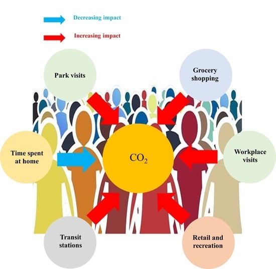
:Quarantining at home during the COVID-19 pandemic significantly restricted human mobility such as visits to parks, grocery stores, workplaces, retail places, and transit stations. In this research, we analyzed how the changes in human mobility during the first wave of the COVID-19 pandemic, from February to April 2020 (i.e., between 17 February and 30 April 2020), affected the daily CO2 emissions for countries having a high number of coronavirus cases at that time. Our daily time-series analyses indicated that when average hours spent at home increased, the amount of daily CO2 emissions declined significantly. The findings suggest that for all three countries (the US, India, and France), a 1% increase in the average duration spent in residential areas reduced daily CO2 emissions by 0.17 Mt, 0.10 Mt, and 0.01 Mt, respectively, during the first wave period. Thus, confining people into their homes contributes to cutting down CO2 emissions remarkably. However, the study also reveals those activities such as visiting parks and going grocery shopping increase CO2 emissions, suggesting that unnecessary human mobility is undesirable for the environment.
1. Introduction
As the Intergovernmental Panel on Climate Change (IPCC) states in its Fifth Assessment Report (AR5), the causes of climate change are largely related to anthropogenic greenhouse gas emissions driven by economic growth and population increases [1]. Thus, the simplest solution to climate change is to stop or restrict human activities. However, this is unrealistic since every country wants to enjoy economic development, and wealth is often related to economic growth. However, the recent spread of the COVID-19 has forced many countries into lockdown and, for the first time after the industrial revolution, almost the entire world is confining people at their homes, restricting human mobility.
The lockdown regulations in many countries are prohibiting people from going out of their homes unless they need to buy necessities at grocery and pharmacy stores. Even going to public parks was restricted in some countries where social distancing was difficult to implement. As human mobility declined during the COVID-19 pandemic, nature is regenerating [2], and this stagnant mobility is likely reducing global greenhouse gas emissions. For example, the global CO2 emissions are claimed to have decreased by 17% during the first quarter of 2020 relative to the mean level of emissions in 2019 [3]. Furthermore, NASA (the National Aeronautics and Space Administration) and ESA (the European Space Agency) reports that during the COVID-19 pandemic, NO2 emissions decreased by up to 30% due to the lockdown restrictions [4].
Although a significant number of studies exist concerning how the COVID-19 crisis is affecting human mobility changes [5], tourism and hospitality [6,7,8], and fuel markets [9], not much is known about how these mobility changes are related to CO2 emissions. The effects of the COVID-19 pandemic on CO2 emissions have been investigated with respect to emission levels [3], air quality index [10], and waste recycling [11]. Some studies examined the effects of lockdown on environmental pollution. However, these studies use the satellite remote sensing datasets [12,13], and no studies have investigated how changes in human mobility during the COVID-19 pandemic are related to CO2 emissions.
Based on Quere et al., [3], which identifies a temporary reduction in daily global CO2 emissions during the COVID-19 pandemic, we hypothesized that capturing the levels of human mobility restriction might have an impact on CO2 emissions levels. Before the COVID-19 pandemic, no reliable data were available to capture a huge decline in human movements where most people spend their time in their houses restricting unnecessary and nonurgent outings and no studies have examined how mobility changes in a country influence its CO2 emissions. Hence, this is the first study to quantitatively investigate the effects of the reduction in human mobility on CO2 emissions. Conducting a social experiment might be an alternative way to obtain such data, but unless a whole city participates in the experiment, it would be very difficult to control the people’s movement within a city. Moreover, even if some cities claimed to participate in such an experiment it would be morally wrong to restrict the residence of the city from moving outside their homes.
Hence, by taking advantage of this opportunity where data that seizes changes in the human mobility under the lockdown are available, this study investigated how human mobility changes during the first wave of COVID-19 affected CO2 emissions. We applied the autoregressive distributed lag (ARDL) model [14] on human mobility indices obtained for the United States (US), India, and France [15]. Since the lockdown’s effect is most likely observable in the number of hours spent at homes, we focus on whether increased hours of stay in residential areas impacted CO2 emissions. Furthermore, since the obtained human mobility data also contain changes in the number of visits to parks, groceries and pharmacies, workplaces, retail and recreational places, and transit stations, we also identify the different impacts on the emission levels among these sectors.
2. CO2 Emissions and Changes in Human Mobility during the COVID-19 First Wave
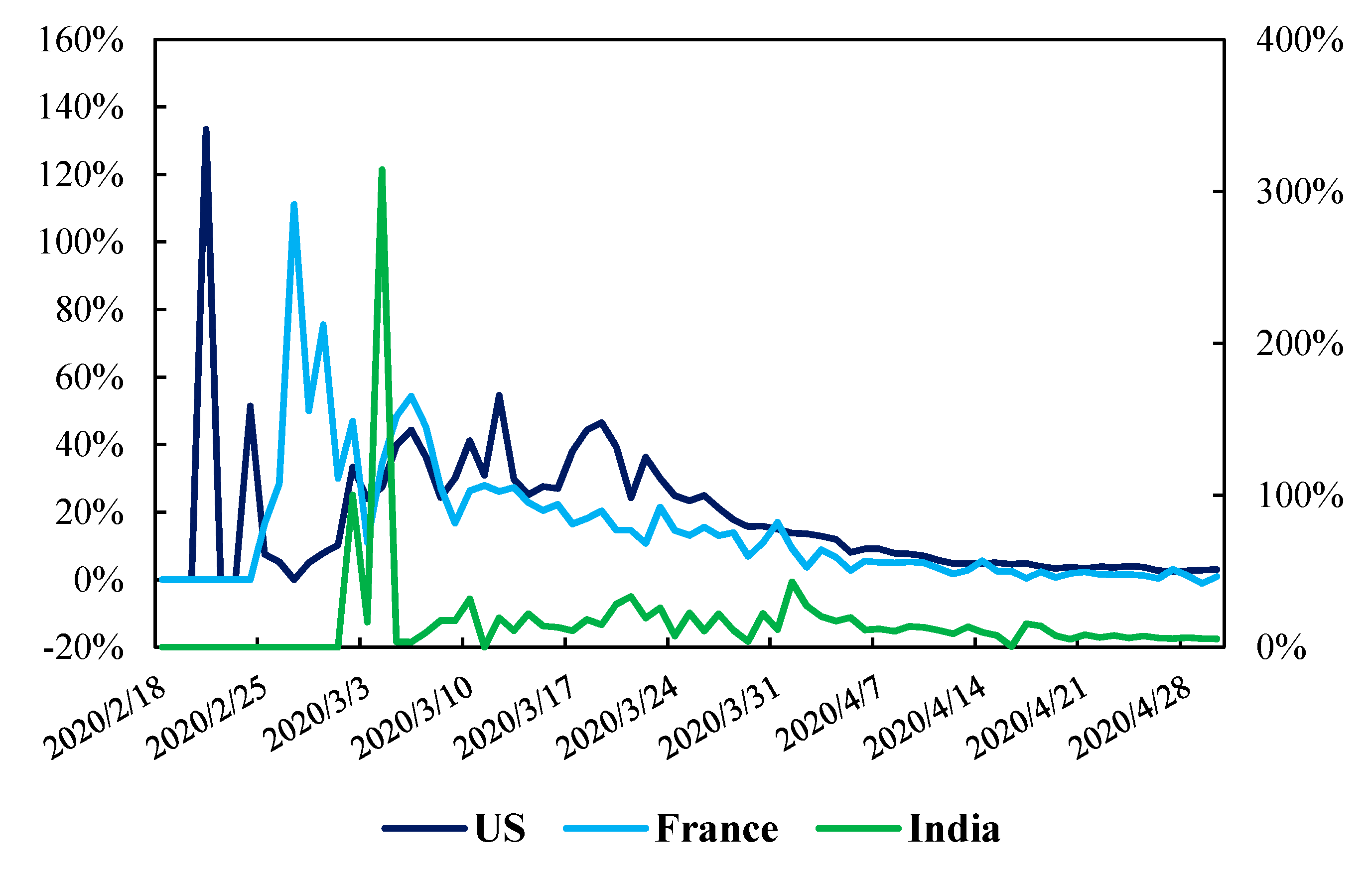
The period investigated in this study contains data between 17 February and 30 April 2020, since this period corresponds to the time when an increasing number of COVID-19 cases began to be identified in various countries outside China (where the first new type of coronavirus epidemic broke out in Wuhan [16]). The study considered three countries having a large number of COVID-19 cases in North America, Asia, and Europe, namely the US, India, and France, respectively. These countries were chosen since they are one of the world’s highly COVID-19-affected countries, as well as the top two CO2 emitting countries [17]. During the period investigated, the US, India, and France had near 1.1 million, 35 thousand, and 130 thousand accumulative number of coronavirus cases [18], respectively, and as a comparison, before severe lockdown restrictions were enforced in these countries in mid-March [19], the daily changes in the number of COVID-19 cases were increasing drastically (Figure 1). By the end of April 2020, the daily changes in the COVID-19 had slowed down (Figure 1) and therefore in this study, the 17 February–30 April 2020 period is defined as the first wave of COVID-19.
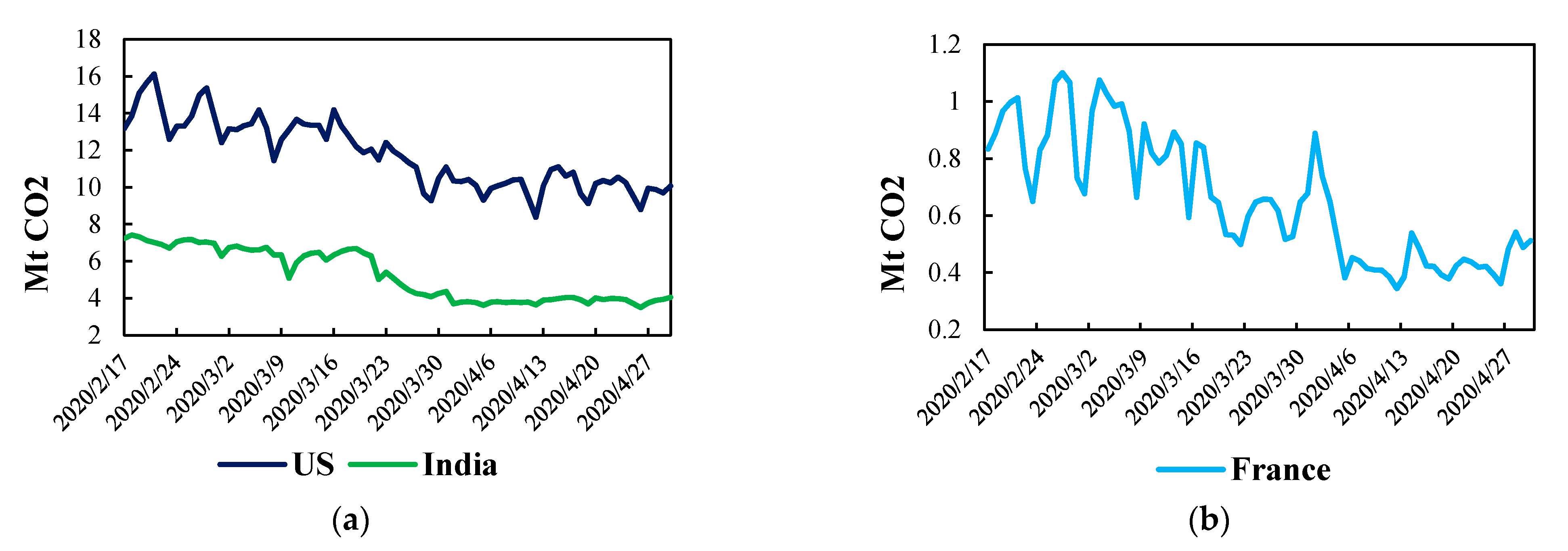
The daily CO2 emissions (Mt CO2) data for the US, India, and France is obtained from the Carbon Monitor [20]. During the COVID-19 first wave (17 February 2020–30 April 2020), the daily CO2 emissions of all three countries investigated had a declining trend (Figure 2a,b). The main purpose of the study is to investigate if this decline in the CO2 emissions during the COVID-19 first wave is related to lockdown restriction by testing the effects of changes in human mobility on the emissions level.
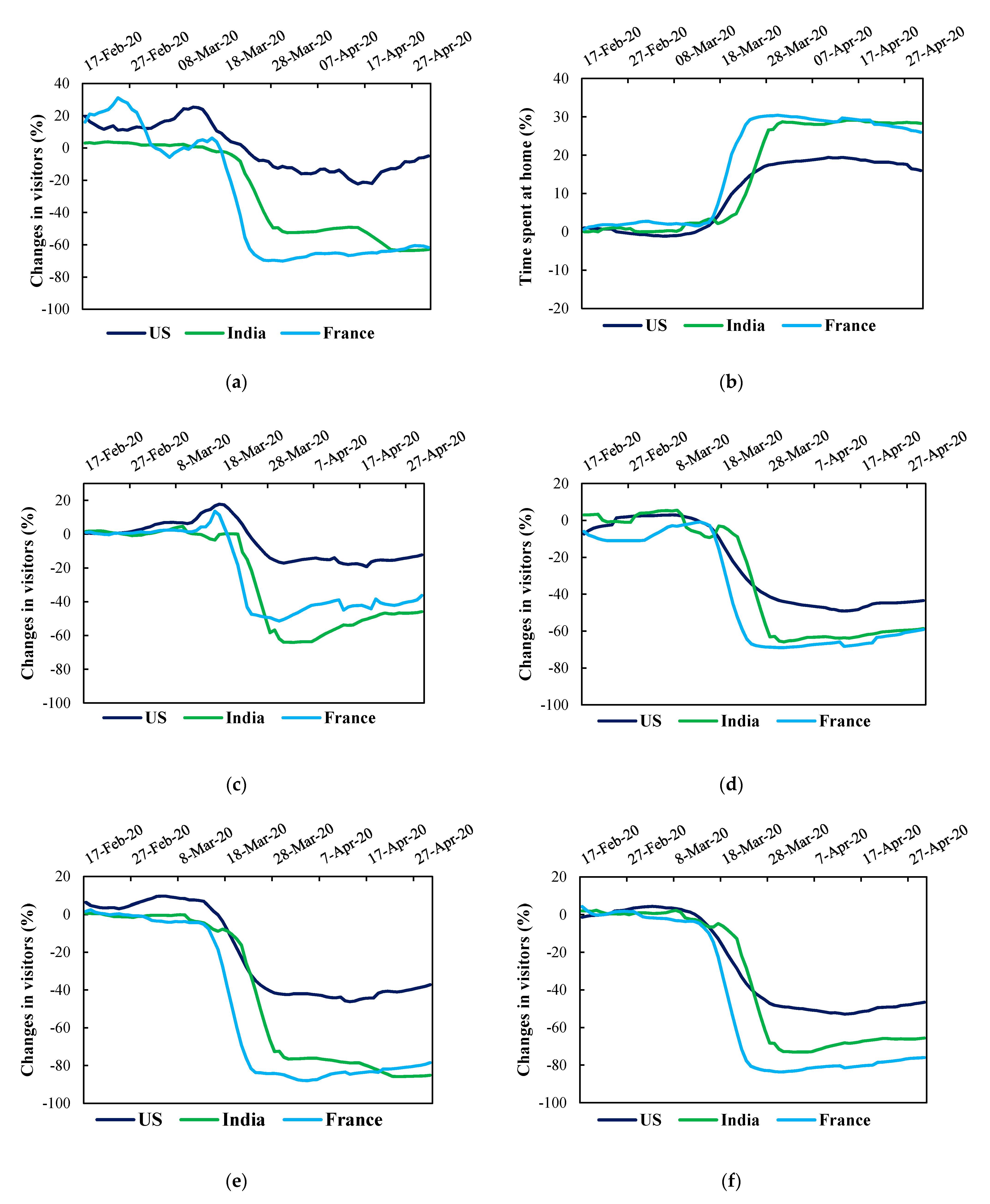
Six human mobility indices were obtained from Google limited liability company (LLC) [15] for the first wave period. The indices represent changes in visits and the number of hours spent at homes relative to a baseline day, where the baseline day is defined as the median value between 3 January and 6 February 2020. The first index is the changes in the visits to parks and outdoor spaces (Figure 3a), and the second is hours spent at home (Figure 3b). The third, fourth, and fifth indices are changes in the number of visits to groceries and pharmacies, workplaces, and retail and recreational places, respectively (Figure 3c–e). Finally, the last index is the changes in the transit station visits (Figure 3f). Except for the residential index, all five mobility indices remained near zero or above zero before enforcing lockdown restrictions (Figure 3a–f). However, when all three countries implemented severe quarantine restrictions after mid-March 2020, all these indices plummeted over 50% (Figure 3a,c–f). On the other hand, time spent at home increased dramatically after mid-March due to the quarantine measures in all three countries (Figure 3b).
3. Materials and Methods
The effects of changes in the human mobility during the first wave of COVID-19 pandemic on the CO2 emissions were analyzed using the following Equations:
where CO2 is the total daily CO2 emissions, park, residential, grocery, work, retail, and transit are the daily human mobility variables included in the Google mobility trends, and COVID are the daily changes in the number of coronavirus cases. Each equation is estimated using the ARDL model with unrestricted intercepts with no trends (Case III) proposed by Pesaran et al., (2001) for the US, India, and France using data from these three countries.
The first reason for using the ARDL model is that this model can be used on time series data even when orders of integration of the test variables are either I (1) or I (0). Testing the long-run relationship between variables in a time series analysis is often conducted by cointegration tests. Many conventional cointegration tests such as the Johansen test [21] require all the test variables to be cointegrated of the same order, but such a condition is not required for the ARDL. The second advantage of the ARDL model is that this model does not lose its power even when omitted variables and autocorrelation issues sustain in the data and, thus, the model is useful for analyzing data with small sample sizes [22].
Since ARDL requires the test variables to be either I (1) or I (0), we applied the Elliott-Rothenberg-Stock (1996) [23], Kwiatkowski–Phillips–Schmidt–Shin (KPSS) [24] tests, and the Lee-Strazicich (2003) [25] test with two structural breaks. Based on the results of one of these tests, we were able to confirm that all our endogenous variables can be considered as either I (1) or I (0) (Table 1).
Second, the ARDL (p, q) model estimation was conducted with the following unrestricted error correction model:
where mobility is one of the six mobility variables investigated in the study, p and q are the lag orders of the dynamic regressors, and εt is the white noise error term.
To test if the models contain serial correlation and heteroskedasticity issues, the Breusch–Godfrey test for autocorrelation [26,27] and the Breusch and Pagan (1979) [28] test for heteroskedasticity and Jarque and Bera (1980) test [29] for normality were performed. The cumulative sum (CUSUM) and the cumulative sum of squares (CUSUMSQ) tests were also conducted to examine the stability of the parameters estimated by the ARDL and non-linear autoregressive distributed lag (NARDL) models.
As observable from the Breusch–Godfrey (BG) test results presented in Table 2, none of our models contained some serial correlation issue under the 5% significance level. The Breusch-Pagan-Godfrey (BPG) test suggested that most of our models are homoscedastic based on the 5% significance level, but the work model for India and the grocery model for France contained heteroscedasticity. To overcome the issues of serial correlation and heteroscedasticity, we used the Newey–West heteroscedasticity and autocorrelation corrected (HAC) standard errors for estimating the ARDL model coefficients. We also investigated the stability of the parameters estimated with the CUSUM and CUSUMQ tests. These details of these results are provided in the supplementary file.
4. Results
4.1. Linear ARDL Bounds Test for Cointegration
A cointegration test was performed using the ARDL bounds test. The results indicated that except for the US and French grocery models, our mobility models for the three countries had cointegration relationships at the 5% significance level (Table 3). Although cointegration relationships were not confirmed for the US and French grocery models by the bounds test, the Johansen cointegration test performed between the CO2 and grocery for the US and French models suggested that they are cointegrated at the 5% significance level (see Table S1 in the Supplementary Materials). Based on this result, the ARDL unrestricted error correction model was estimated, capturing both short-run and long-run relationships between the CO2 emissions and human mobility indices.
4.2. Staying Home Is Cutting Down CO2 Emissions
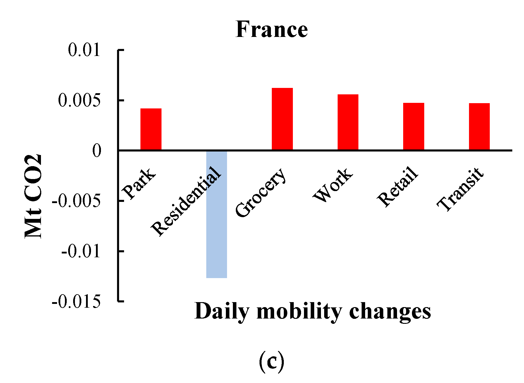
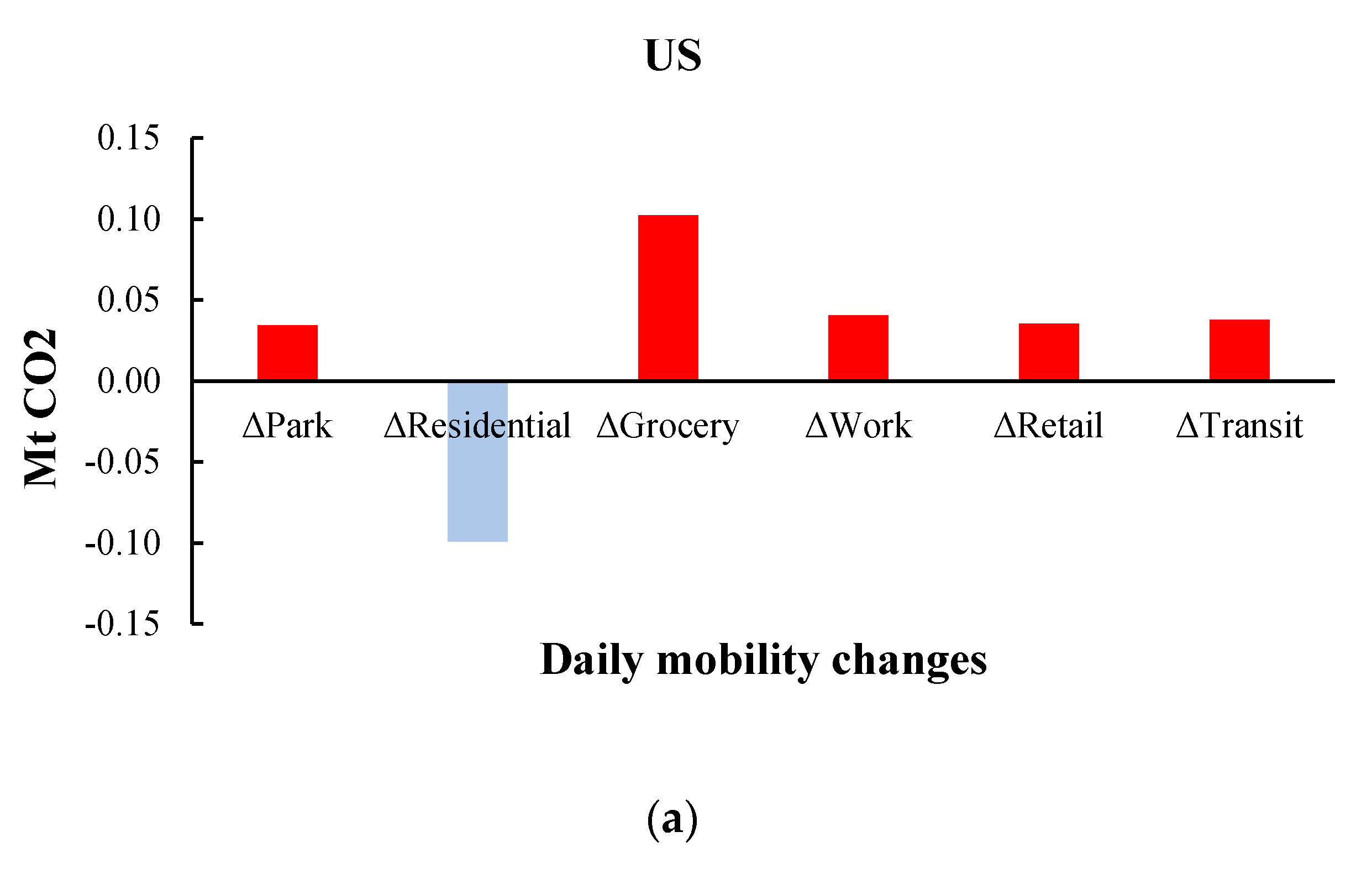
Investigating how daily changes in the number of hours spent at residential areas influence the daily CO2 emissions, a 1% increase in the time spent at home in the US, India, and France resulted in a 0.1 Mt, 0.25 Mt, and 0.006 Mt reduction in CO2 emissions, respectively (Figure 4a–c, Table 4). These results indicate that since more people were forced to stay at their homes during the quarantine, it is probable that the use of automobiles and aircraft in their daily lives declined, resulting in a reduction of carbon emissions [30,31].
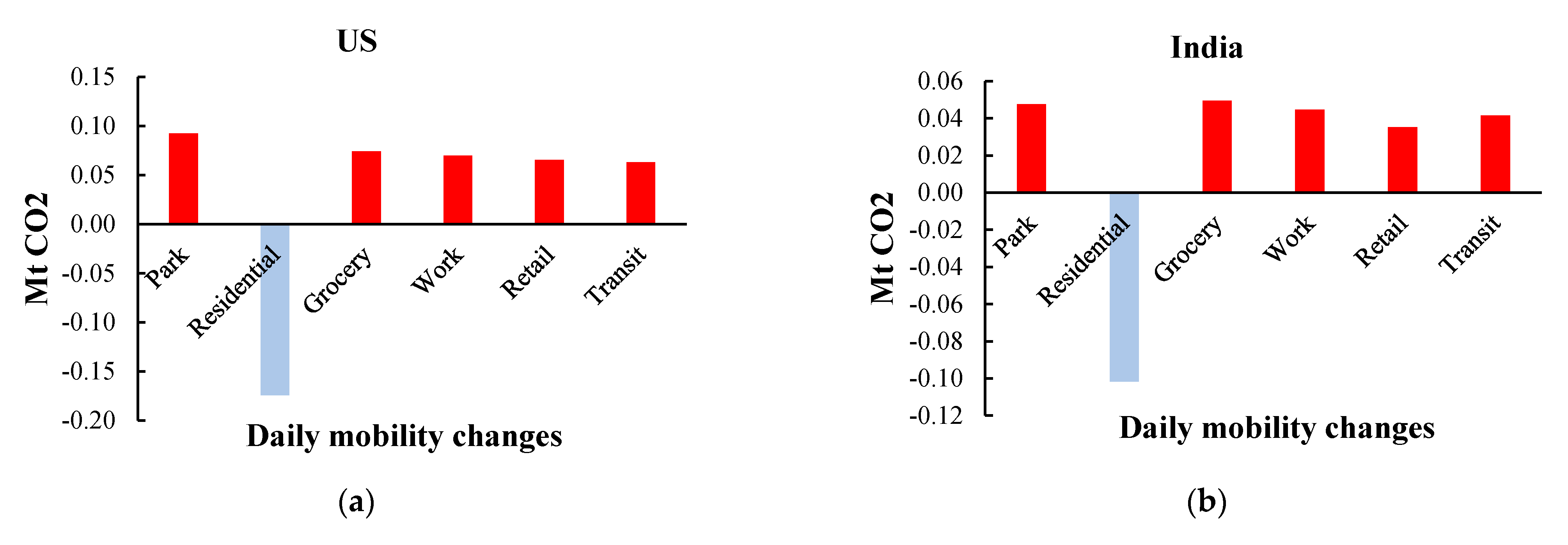
The long-run coefficients of the ARDL model also reveal that in all three countries, increased hours spent at home contribute to reducing CO2 emissions (Figure 5a–c, Table 5). Our result implies that a 1% increase in the residential index reduced daily CO2 emissions by 0.17 Mt, 0.10 Mt, and 0.01 Mt in the US, India, and France, respectively (Figure 5a–c, Table 5). The difference in the size of the CO2 reductions from staying at home longer among the three countries reflects the total volume of CO2 emissions. The US and India are ranked the second and third after China while France is ranked the 19th for its annual CO2 emissions in the world [17].
These results indicate that constraining people at their homes during the COVID-19 pandemic contributed to reducing CO2 emissions. This implies that such a policy that restricts people to stay at their homes for hours might help decrease CO2 emissions.
4.3. Parks, Groceries, and Workplace Visits Contributing to CO2 Emissions
During the lockdown restrictions, many countries did not prohibit people from going to parks and grocery and pharmacy shopping if social distancing was possible. The park index used in the study contained parks such as local and national parks, public beaches, marina, dog parks, and so on, and the grocery index “includes places such as grocery markets, food warehouses, farmers markets” [15] and so on. The short-run results for the US, India, and France model suggests that a 1% increase in the daily park and grocery mobility indices raised the US daily CO2 emissions by 0.03 Mt and 0.1 Mt, those for India by 0.12 Mt and 0.09 Mt, and France for 0.002 Mt and 0.002 Mt, respectively (Figure 4a–c, Table 4). The effects of mobility changes in parks and groceries during the entire first wave period show that visits to groceries had the highest contribution to CO2 emissions for India and France, and it was the second-highest for the US (Figure 5a–c). In the US, India, and France, a 1% increase in grocery visits lead to a 0.07 Mt, 0.05 Mt, and 0.006 Mt increase in the CO2 emissions (Figure 5a–c, Table 5). This is expected, since even the number of visits to groceries and pharmacies declined during the quarantine (Figure 3c), people had to continue to go shopping at grocery stores, but this activity often involves using automobiles. The park visits also impacted largely on daily CO2 emissions for the US and India. It had the largest influence on the emissions for the US rising 0.09 Mt, and it had the second-largest impact on the emissions for India. For France, the increase in the emissions from park visits was relatively small among the other five mobility indices rising CO2 emissions (Figure 5c). We predict that this is related to French citizens using bicycles or walking in order to visit parks, while the US citizens usually use their car [32].
Finally, although most countries promoted companies to shift to working from home, it was impossible to stop people from going to offices entirely. Even if the number of workers visiting their offices declined during the quarantine, if some people continued to work at their office buildings, electricity to warm the buildings and other utilities to run the office contributed to energy use. However, in general, it is still uncertain whether working at home is better than the office in terms of CO2 emissions since the total amount of emissions varies by way of commuting and distance to the office [33].
4.4. Retail & Recreation and Transport Station Mobility Contributing to CO2 Emissions
The study found that an increase in the visits to retail and recreational places and transit stations also positively impacted CO2 emissions. When the number of visitors to retail and recreational places and transit stations increased by 1% during the first wave, the CO2 emissions grew by 0.065 Mt and 0.063 Mt for the US, 0.035 Mt and 0.042 Mt for India, and 0.005 Mt and 0.005 Mt for France, respectively (Figure 5a–c, Table 5). Since the retail and recreational index was based on the number of visits to restaurants, cafes, shopping centers, theme parks, museums, libraries, and movie theaters, an increase in visits to these places will add the volume of gasoline to travel to these places and energy to run their facilities. Hence, an increase in this mobility index will likely increase CO2 emissions. Similarly, an increase in transit station visits reflects conditions in which more people are taking public transportation to various destinations. Thus, an increase in human mobility in transit stations will contribute to CO2 emissions positively.
Higher human mobility in the retail and recreational places and transit stations signifies a condition where more people enjoy their commercial lifestyle before the pandemic. Hence, the results of these mobility indices showing a positive effect on CO2 emissions means that CO2 emissions will increase as peoples’ lives return to normal without experiencing the effects of lockdowns.
4.5. Practical Implications
Although the restrictions imposed on human movement during COVID-19 were not meant to reduce CO2 emissions, both the long-run and short-run results of our ARDL estimations revealed that confining people in their homes for a longer period contributes to reducing CO2 emissions. Since our short-run results indicate that even a daily increase in the hours spent at homes has a negative impact on CO2 emissions, it implies that any policy that will keep people in their homes for a longer period can help reduce CO2 emissions. Thus, introducing a holiday at a global level that will restrict people to stay at their homes to reduce CO2 might be a practical way to realize the effects of our findings.
Another intriguing result is that those activities not being restricted under the lockdown policy in most countries such as going grocery shopping and visiting parks tended to have a larger impact on the CO2 emissions compared to those that have been more or less restricted under the policy such as visits to retail and recreational places when analyzed regarding the daily change in the mobility. This implies that activities that will increase human mobility can lead to an increase in CO2 emissions and have a higher contribution to CO2 emissions compared to the case when people are kept at their homes.
5. Conclusions
This study evaluated how changes in human mobility during the first wave of COVID-19 affected CO2 emissions by using this opportunity where data that captures changes in human mobility under lockdown are available. For the US, India, and France, six Google mobility indices were used to analyze the consequences of human movement restrictions owing to the COVID-19 pandemic. In this regard, the ARDL unconstrained error correction model was used to predict the short and long-run relationships between CO2 emissions and human mobility indices. Both the short-run and long-run coefficients of the ARDL model reveal that in all three countries, staying home during the COVID-19 first wave cuts off impacts on CO2 emissions, while even necessary outings such as grocery shopping and going to parks contributed to increased CO2 emissions.
Hence, our study finds that restricting peoples’ activities is good for the environment, although such a policy is not realistic to be continued forever. However, it might be possible to have a global policy such as keeping people in their homes for a certain period of a year to control CO2 emissions. During the pandemic, many people must have realized how many of the activities we have been performing before the pandemic are unnecessary. Hence, a policy that at least reduces such unnecessary activities might help decrease CO2 emissions.
The COVID-19 has reduced human mobility across the world due to lockdown regulations, but we have gained a changed world with a better atmosphere. There is no question that once the world engine begins to run after COVID-19, emissions and waste will begin to pile up, posing threats not just to human health but also to environmental sustainability. However, we should learn from the pandemic that reducing human activities is one way to reduce our impact on the environment.
Supplementary Materials
The following are available online at https://0-www-mdpi-com.brum.beds.ac.uk/article/10.3390/su13158534/s1, Table S1: Johansen cointegration tests for the US and France grocery models, Figure S1: CUSUM test for the US model, Figure S2. CUSUM of Squares test for the US model, Figure S3: CUSUM test for the India model, Figure S4: CUSUM of Squares test for the India model, Figure S5: CUSUM test for the France model, Figure S6: CUSUM of Squares test for the France model.
Author Contributions
Conceptualization, K.A., M.M.I. and A.J.; methodology, K.A.; formal analysis, K.A.; data curation, K.A., M.M.I. and A.J.; writing—original draft preparation, K.A., M.M.I. and A.J.; writing—review and editing, K.A., M.M.I. and A.J.; supervision, K.A. All authors have read and agreed to the published version of the manuscript.
Funding
This research received no external funding.
Institutional Review Board Statement
Not applicable.
Informed Consent Statement
Not applicable.
Data Availability Statement
Daily CO2 emissions for the US, India, and France are available at https://carbonmonitor.org (accessed on 8 April 2021). The data for the daily changes in the human mobility data are available at https://ourworldindata.org/covid-google-mobility-trends (accessed on 22 April 2021). The data for the number of COVID-19 cases are available at https://www.worldometers.info/coronavirus (accessed on 4 April 2021).
Acknowledgments
This research received no specific grant from any funding agency in the public, commercial, or not-for-profit sectors.
Conflicts of Interest
The authors declare no conflict of interest.
References
- IPCC. Climate Change 2014: Synthesis Report; IPCC: Geneva, Switzerland, 2014. [Google Scholar]
- Beth, G. Why COVID-19 Will End Up Harming the Environment (National Geography). National Geography. 19 June 2020. Available online: https://www.nationalgeographic.com/science/article/why-covid-19-will-end-up-harming-the-environment (accessed on 13 April 2021).
- Le Quéré, C.; Jackson, R.B.; Jones, M.W.; Smith, A.; Abernethy, S.; Andrew, R.M.; De-Gol, A.J.; Willis, D.R.; Shan, Y.; Canadell, J.G.; et al. Temporary reduction in daily global CO2 emissions during the COVID-19 forced confinement. Nat. Clim. Chang. 2020, 10, 647–653. [Google Scholar] [CrossRef]
- NASA Satellite Data Show 30 Percent Drop in Air Pollution Over Northeast U.S. NASA Air Quality Analysis. 2020. Available online: https://airquality.gsfc.nasa.gov/ (accessed on 16 April 2021).
- Hadjidemetriou, G.M.; Sasidharan, M.; Kouyialis, G.; Parlikad, A.K. The impact of government measures and human mobility trend on COVID-19 related deaths in the UK. Transp. Res. Interdiscip. Perspect. 2020, 6, 100167. [Google Scholar] [CrossRef]
- Hoque, A.; Shikha, F.A.; Hasanat, M.W.; Arif, I.; Hamid, A.B.A. The effect of Coronavirus (COVID-19) in the tourism industry in China. Asian J. Multidiscip. Stud. 2020, 3, 52–58. [Google Scholar]
- Kaushal, V.; Srivastava, S. Hospitality and tourism industry amid COVID-19 pandemic: Perspectives on challenges and learnings from India. Int. J. Hosp. Manag. 2021, 92, 102707. [Google Scholar] [CrossRef] [PubMed]
- Gössling, S.; Scott, D.; Hall, C.M. Pandemics, tourism and global change: A rapid assessment of COVID-19. J. Sustain. Tour. 2020, 29, 1–20. [Google Scholar] [CrossRef]
- Aruga, K. Changes in Human Mobility under the COVID-19 Pandemic and the Tokyo Fuel Market. J. Risk Financ. Manag. 2021, 14, 163. [Google Scholar] [CrossRef]
- Zambrano-Monserrate, M.A.; Ruano, M.A.; Sanchez-Alcalde, L. Indirect effects of COVID-19 on the environment. Sci. Total Environ. 2020, 728, 138813. [Google Scholar] [CrossRef] [PubMed]
- Liu, Z.; Ciais, P.; Deng, Z.; Lei, R.; Davis, S.J.; Feng, S.; Zheng, B.; Cui, D.; Dou, X.; Zhu, B.; et al. Near-real-time monitoring of global CO2 emissions reveals the effects of the COVID-19 pandemic. Nat. Commun. 2020, 11, 1–12. [Google Scholar] [CrossRef]
- Muhammad, S.; Long, X.; Salman, M. COVID-19 pandemic and environmental pollution: A blessing in disguise? Sci. Total Environ. 2020, 728, 138820. [Google Scholar] [CrossRef]
- Fan, C.; Li, Y.; Guang, J.; Li, Z.; Elnashar, A.; Allam, M.; De Leeuw, G. The Impact of the Control Measures during the COVID-19 Outbreak on Air Pollution in China. Remote. Sens. 2020, 12, 1613. [Google Scholar] [CrossRef]
- Pesaran, M.H.; Shin, Y.; Smithc, R.J. Bounds testing approaches to the analysis of level relationships. J. Appl. Econ. 2001, 16, 289–326. [Google Scholar] [CrossRef]
- Google COVID-19 Community Mobility Reports. Google LLC, 2021. Available online: https://www.google.com/covid19/mobility/ (accessed on 22 April 2021).
- Zhu, H.; Wei, L.; Niu, P. The novel coronavirus outbreak in Wuhan, China. Glob. Heal. Res. Policy 2020, 5, 1–3. [Google Scholar] [CrossRef] [PubMed]
- Union of Concerned Scientists. Each Country’s Share of CO2 Emissions. 2020. Available online: https://www.ucsusa.org/resources/each-countrys-share-co2-emissions (accessed on 19 April 2020).
- Worldometer. COVID-19 Coronavirus Pandemic. 2020. Available online: https://www.worldometers.info/coronavirus/ (accessed on 4 April 2021).
- Singh, K.D.; Goel, V.; Kumar, H.; Gettleman, J. India, Day 1: World’s Largest Coronavirus Lockdown Begins. The New York Times. 25 March 2020. Available online: https://www.nytimes.com/2020/03/25/world/asia/india-lockdown-coronavirus.html (accessed on 20 April 2021).
- Carbon Monitor. Carbon Monitor, Near-Real-Time Daily Datasets of Global and Regional CO2 Emissions from Fossil Fuel and Cement Production. 2020. Available online: https://0-doi-org.brum.beds.ac.uk/10.1038/s41467-020-18922-7 (accessed on 8 April 2021).
- Johansen, S. A statistical analysis of cointegration for I(2) variables. Econom. Theory 1995, 11, 25–29. [Google Scholar] [CrossRef]
- Nyga-Łukaszewska, H.; Aruga, K. Energy Prices and COVID-Immunity: The Case of Crude Oil and Natural Gas Prices in the US and Japan. Energies 2020, 13, 6300. [Google Scholar] [CrossRef]
- Elliott, G.; Rothenberg, T.J.; Stock, J.H. Efficient Tests for an Autoregressive Unit Root. Econometrica 1996, 64, 813. [Google Scholar] [CrossRef]
- Kwiatkowski, D.; Phillips, P.C.; Schmidt, P.; Shin, Y. Testing the null hypothesis of stationarity against the alternative of a unit root: How sure are we that economic time series have a unit root? J. Econ. 1992, 54, 159–178. [Google Scholar] [CrossRef]
- Lee, J.; Strazicich, M.C. Minimum Lagrange Multiplier Unit Root Test with Two Structural Breaks. Rev. Econ. Stat. 2003, 85, 1082–1089. [Google Scholar] [CrossRef]
- Breusch, T.S. Testing for Autocorrelation in Dynamic Linear Models*. Aust. Econ. Pap. 1978, 17, 334–355. [Google Scholar] [CrossRef]
- Godfrey, L.G. Testing Against General Autoregressive and Moving Average Error Models when the Regressors Include Lagged Dependent Variables. Econometrica 1978, 46, 1293. [Google Scholar] [CrossRef]
- Breusch, T.S.; Pagan, A.R. A Simple Test for Heteroscedasticity and Random Coefficient Variation. Econometrica 1979, 47, 1287. [Google Scholar] [CrossRef]
- Jarque, C.M.; Bera, A.K. Efficient tests for normality, homoscedasticity and serial independence of regression residuals. Econ. Lett. 1980, 6, 255–259. [Google Scholar] [CrossRef]
- Liu, M.; Tan, S.; Zhang, M.; He, G.; Chen, Z.; Fu, Z.; Luan, C. Waste paper recycling decision system based on material flow analysis and life cycle assessment: A case study of waste paper recycling from China. J. Environ. Manag. 2020, 255, 109859. [Google Scholar] [CrossRef] [PubMed]
- Yusup, Y.; Ramli, N.; Kayode, J.; Yin, C.; Hisham, S.; Isa, H.M.; Ahmad, M. Atmospheric Carbon Dioxide and Electricity Production Due to Lockdown. Sustainability 2020, 12, 9397. [Google Scholar] [CrossRef]
- De Vos, J. The effect of COVID-19 and subsequent social distancing on travel behavior. Transp. Res. Interdiscip. Perspect. 2020, 5, 100121. [Google Scholar] [CrossRef] [PubMed]
- Crow, D.; Millot, A. Working from Home Can Save Energy and Reduce Emissions. But How Much? 2021. Available online: https://www.iea.org/commentaries/working-from-home-can-save-energy-and-reduce-emissions-but-how-much (accessed on 23 April 2021).
Figure 1.
Trends of COVID-19 during the first wave of the pandemic (17 February 2020–30 April 2020). The left vertical axis shows the percentage changes of COVID-19 cases for the US and France, while the right shows those for India.
Figure 1.
Trends of COVID-19 during the first wave of the pandemic (17 February 2020–30 April 2020). The left vertical axis shows the percentage changes of COVID-19 cases for the US and France, while the right shows those for India.

Figure 2.
Trends of CO2 emissions during the first wave of the COVID-19 pandemic (17 February 2020–30 April 2020). (a) The US and India. (b) France. The vertical axis shows the daily CO2 emissions (Mt CO2). Changes in CO2 emissions are accumulated from the power (±1.5%), ground transport (±9.3%), industry (±36.0%), residential (±40.0%), and domestic aviation (±10.2%) with an overall uncertainty of ±6.8%.

Figure 3.
Google mobility trends during the first wave of the COVID-19 pandemic (17 February 2020–30 April 2020). The figure presents changes in the six mobility indices: (a) Parks and outdoor spaces. (b) Time spent at home (Residential). (c) Groceries and pharmacies. (d) Workplaces. (e) Retail and recreation. (f) Public transport stations (Transit) in the US (navy line), India (green line), and France (blue line).

Figure 4.
Effects of daily changes in mobility indices on the daily CO2 emissions. The graph shows the short-run coefficients of the ARDL model estimation. (a) The US. (b) India. (c) France. All coefficients are significant at the 5% level except for the US grocery coefficient.
Figure 4.
Effects of daily changes in mobility indices on the daily CO2 emissions. The graph shows the short-run coefficients of the ARDL model estimation. (a) The US. (b) India. (c) France. All coefficients are significant at the 5% level except for the US grocery coefficient.

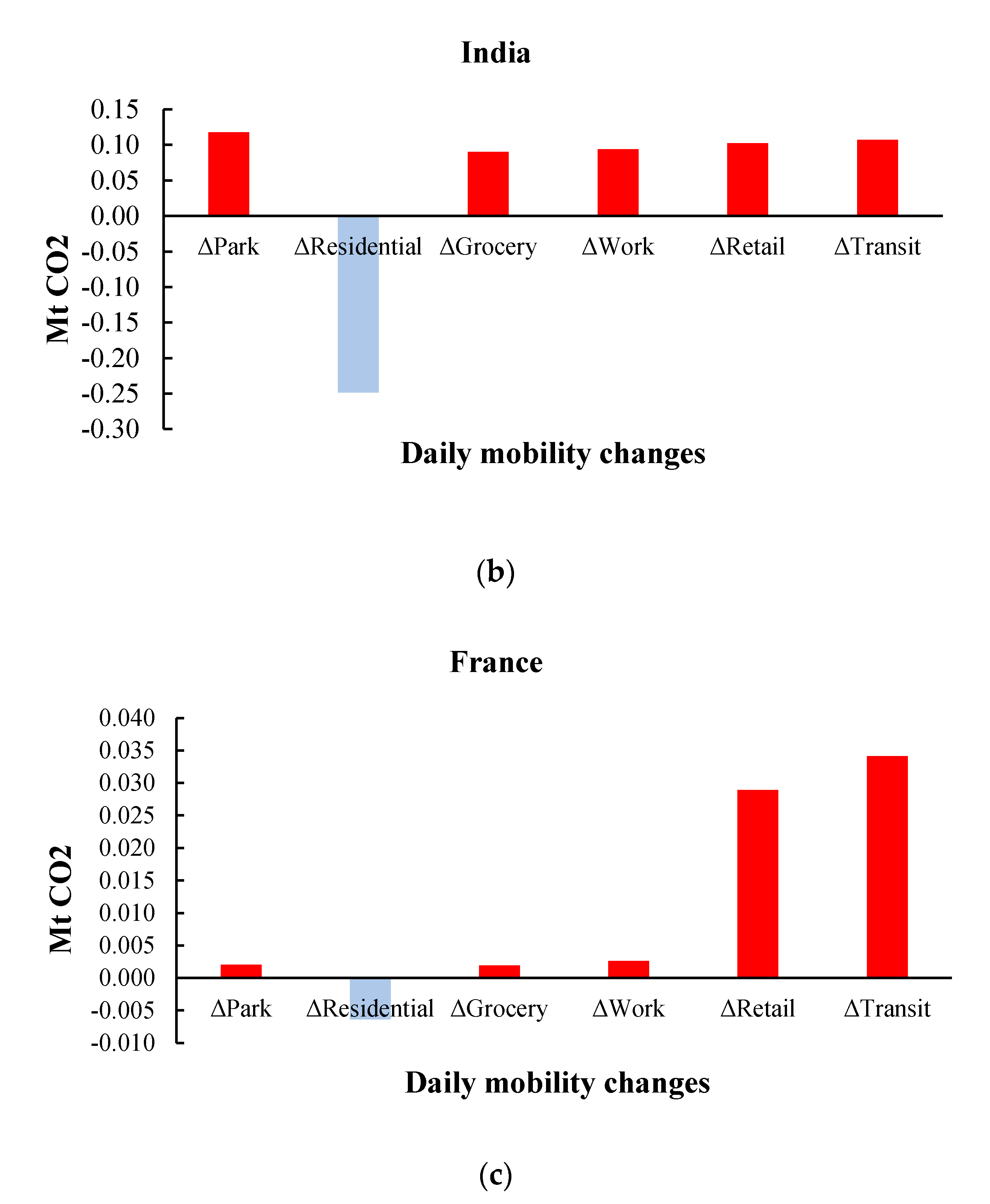
Figure 5.
Effects of mobility changes on the daily CO2 emissions during the first wave of the COVID-19 pandemic (17 February 2020–30 April 2020). (a) The US. (b) India. (c) France. The vertical axis shows the increase or decrease in the daily CO2 emissions when the six mobility indices change by 1% based on the ARDL estimation. In addition, the graph shows the long-run coefficients of the ARDL model, all significant at the 5% level.


Table 1.
Unit root tests.
| Variables | Levels | First Differences | ||||||||||
|---|---|---|---|---|---|---|---|---|---|---|---|---|
| ERS | KPSS | LS | ERS | KPSS | LS | |||||||
| US CO2 | 2.71 | *** | 0.17 | * | −5.09 | 42.15 | 0.19 | ** | −6.52 | ** | ||
| US park | 5.69 | * | 0.13 | * | −4.61 | 8.58 | 0.14 | * | −7.51 | *** | ||
| US residential | 2.58 | *** | 0.16 | ** | −5.58 | 12.47 | 0.20 | ** | −6.40 | ** | ||
| US grocery | 6.17 | * | 0.14 | * | −7.70 | *** | 6.47 | * | 0.11 | −7.40 | *** | |
| US work | 7.38 | 0.15 | ** | −6.07 | * | 26.13 | 0.22 | *** | −7.53 | *** | ||
| US retail | 4.92 | ** | 0.15 | ** | −7.32 | *** | 12.77 | 0.16 | ** | −7.01 | *** | |
| US transit | 3.02 | *** | 0.16 | ** | −8.57 | *** | 34.02 | 0.21 | ** | −7.58 | *** | |
| India CO2 | 9.59 | 0.14 | * | −5.51 | 2.93 | *** | 0.09 | −10.75 | *** | |||
| India park | 3.65 | *** | 0.12 | −7.87 | *** | 1.82 | *** | 0.11 | −7.43 | *** | ||
| India residential | 4.32 | ** | 0.13 | * | −9.50 | *** | 2.07 | *** | 0.14 | * | −10.30 | *** |
| India grocery | 2.70 | *** | 0.14 | * | −7.05 | *** | 8.48 | 0.13 | * | −10.56 | *** | |
| India work | 9.38 | 0.14 | * | −7.85 | *** | 5.93 | * | 0.13 | * | −9.29 | *** | |
| India retail | 4.11 | *** | 0.13 | * | −10.26 | *** | 1.88 | *** | 0.14 | * | −11.54 | *** |
| India transit | 3.99 | *** | 0.14 | * | −8.79 | *** | 2.77 | *** | 0.14 | * | 10.92 | *** |
| France CO2 | 2.73 | *** | 0.11 | −6.21 | * | 12.73 | 0.20 | ** | −6.64 | ** | ||
| France park | 8.37 | 0.19 | * | −10.41 | *** | 0.48 | *** | 0.10 | −6.81 | ** | ||
| France residential | 3.81 | *** | 0.16 | * | −9.51 | ** | 2.86 | *** | 0.12 | * | −9.45 | *** |
| France grocery | 8.79 | 0.14 | * | −7.87 | ** | 4.75 | ** | 0.10 | −10.53 | *** | ||
| France work | 7.11 | 0.15 | ** | −9.66 | *** | 2.10 | *** | 0.11 | −8.91 | *** | ||
| France retail | 26.05 | 0.18 | ** | −11.40 | *** | 1.36 | *** | 0.13 | * | −8.54 | *** | |
| France transit | 7.78 | 0.17 | ** | −14.95 | *** | 3.93 | *** | 0.12 | * | −9.97 | *** | |
Note: ***, **, and * denote significance at the 1%, 5%, and 10% levels, respectively. ERS is the Elliott-Rothenberg-Stock (1996) test, and LS is the Lee-Strazicich (2003) test with two structural breaks. The null hypothesis of the ERS and LS tests are variables that contain unit roots, while that for the KPSS test is stationarity of the variables.
Table 2.
Serial correlation and heteroscedasticity tests.
| Models | US | India | France | |||||||||||
|---|---|---|---|---|---|---|---|---|---|---|---|---|---|---|
| BG | BPG | JB | BG | BPG | JB | BG | BPG | JB | ||||||
| Park | 0.54 | 1.79 | 1.17 | 0.50 | 0.52 | 142.33 | *** | 0.10 | 2.42 | * | 4.54 | |||
| Residential | 0.12 | 1.72 | 0.28 | 0.18 | 1.34 | 102.90 | *** | 0.09 | 2.08 | * | 3.38 | |||
| Grocery | 2.19 | * | 1.37 | 1.85 | 0.31 | 0.40 | 59.15 | *** | 1.03 | 3.16 | ** | 1.34 | ||
| Work | 0.15 | 1.53 | 0.43 | 1.04 | 3.13 | *** | 30.53 | *** | 0.07 | 2.30 | * | 2.69 | ||
| Retail | 0.11 | 1.70 | 0.49 | 0.55 | 0.82 | 145.83 | *** | 0.30 | 1.24 | 6.19 | ** | |||
| Transit | 0.08 | 1.62 | 0.38 | 0.16 | 0.70 | 155.65 | *** | 0.08 | 1.68 | 9.11 | ** | |||
Note: ***, **, and * denote significance at the 1%, 5%, and 10% levels, respectively.
Table 3.
ARDL bounds test for cointegration.
| Models | US | India | France | |||
|---|---|---|---|---|---|---|
| F-Stat. | F-Stat. | F-Stat. | ||||
| Park | 6.38 | *** | 4.74 | ** | 6.29 | *** |
| Residential | 11.23 | *** | 8.33 | *** | 6.67 | *** |
| Grocery | 3.74 | * | 4.44 | ** | 3.48 | |
| Work | 11.23 | *** | 8.11 | *** | 5.96 | *** |
| Retail | 10.36 | *** | 5.87 | ** | 8.34 | *** |
| Transit | 11.82 | *** | 8.24 | *** | 8.10 | *** |
| Significance level | I (0) | I (1) | ||||
| 1% level | 5.16 | 5.96 | ||||
| 5% level | 3.78 | 4.33 | ||||
| 10% level | 3.13 | 3.62 | ||||
Note: ***, **, and * denote significance at the 1%, 5% and 10% levels, respectively.4.2. Staying Home is Cutting Down CO2 Emissions.
Table 4.
ARDL short-run estimations.
| Models | Variables | US | India | France | ||||||
|---|---|---|---|---|---|---|---|---|---|---|
| Coefficient | Std. Error | Coefficient | Std. Error | Coefficient | Std. Error | |||||
| Park | ΔPark | 0.0344 | *** | 0.0108 | 0.1178 | *** | 0.0311 | 0.0020 | *** | 0.0006 |
| ΔPark(-1) | na | −0.0678 | ** | 0.0314 | na | |||||
| Covid | 0.6571 | 0.4915 | −0.0491 | 0.0838 | 0.1001 | 0.0820 | ||||
| Residential | ΔResidential | −0.0992 | *** | 0.0207 | −0.2482 | *** | 0.0528 | −0.0063 | *** | 0.0018 |
| ΔResidential (-1) | na | 0.0424 | 0.0639 | na | ||||||
| ΔResidential (-2) | na | 0.0050 | 0.0618 | na | ||||||
| ΔResidential (-3) | na | 0.0886 | 0.0533 | na | ||||||
| Covid | 0.7707 | 0.4488 | −0.0357 | 0.0800 | 0.0817 | 0.0815 | ||||
| Grocery | ΔGrocery | 0.1021 | * | 0.0600 | 0.0901 | *** | 0.0159 | 0.0019 | ** | 0.0009 |
| ΔGrocery (-1) | na | −0.0138 | 0.0176 | na | ||||||
| ΔGrocery (-2) | na | −0.0090 | 0.0169 | na | ||||||
| ΔGrocery (-3) | na | −0.0404 | ** | 0.0160 | na | |||||
| Covid | 0.9264 | * | 0.5276 | −0.0276 | 0.0805 | 0.0582 | 0.0836 | |||
| Work | ΔWork | 0.0406 | *** | 0.0085 | 0.0940 | *** | 0.0172 | 0.0026 | *** | 0.0008 |
| ΔWork (-1) | na | −0.0231 | 0.0210 | na | ||||||
| ΔWork (-2) | na | −0.0063 | 0.0205 | na | ||||||
| ΔWork (-3) | na | −0.0298 | * | 0.0176 | na | |||||
| Covid | 0.7187 | 0.4498 | −0.0554 | 0.0787 | 0.0774 | 0.0826 | ||||
| Retail | ΔRetail | 0.0354 | *** | 0.0078 | 0.1020 | *** | 0.0224 | 0.0289 | ** | 0.0118 |
| ΔRetail (-1) | na | −0.0567 | ** | 0.0228 | −0.0265 | ** | 0.0117 | |||
| Covid | 0.7546 | 0.4552 | −0.0487 | 0.0796 | 0.0666 | 0.0789 | ||||
| Transit | ΔTransit | 0.0376 | *** | 0.0076 | 0.1072 | *** | 0.0215 | 0.0341 | ** | 0.0137 |
| ΔTransit (-1) | na | −0.0323 | 0.0264 | −0.0302 | ** | 0.0136 | ||||
| ΔTransit (-2) | na | 0.0018 | 0.0255 | na | ||||||
| ΔTransit (-3) | na | −0.0456 | ** | 0.0220 | na | |||||
| Covid | 0.7945 | * | 0.4446 | −0.0273 | 0.0769 | 0.0853 | 0.0792 | |||
Note: ***, **, and * denote significance at the 1%, 5%, and 10% levels, respectively. na in the table implies that the statistically feasible models chosen by the AIC (Akaike information criterion) did not contain the lags of the variables.
Table 5.
ARDL long-run estimations.
| Models | Variables | US | India | France | ||||||
|---|---|---|---|---|---|---|---|---|---|---|
| Coefficient | Std. Error | Coefficient | Std. Error | Coefficient | Std. Error | |||||
| Park | Constant | 11.3930 | *** | 0.4047 | 6.5396 | *** | 0.1455 | 0.7611 | *** | 0.0450 |
| Park | 0.0925 | *** | 0.0209 | 0.0475 | *** | 0.0035 | 0.0042 | *** | 0.0007 | |
| Residential | Constant | 13.2505 | *** | 0.4169 | 6.7291 | *** | 0.1175 | 0.8523 | *** | 0.0590 |
| Residential | −0.1741 | *** | 0.0214 | −0.1016 | *** | 0.0045 | −0.0126 | *** | 0.0024 | |
| Grocery | Constant | 11.1546 | *** | 0.5478 | 6.4515 | *** | 0.1828 | 0.7633 | *** | 0.0886 |
| Grocery | 0.0740 | ** | 0.0317 | 0.0494 | *** | 0.0037 | 0.0062 | *** | 0.0022 | |
| Work | Constant | 13.2533 | *** | 0.4187 | 6.6252 | *** | 0.1154 | 0.8567 | *** | 0.0731 |
| Work | 0.0699 | *** | 0.0085 | 0.0447 | *** | 0.0020 | 0.0056 | *** | 0.0012 | |
| Retail | Constant | 12.8352 | *** | 0.4101 | 6.7385 | *** | 0.1427 | 0.8748 | *** | 0.0400 |
| Retail | 0.0653 | *** | 0.0089 | 0.0353 | *** | 0.0020 | 0.0047 | *** | 0.0006 | |
| Transit | Constant | 13.2069 | *** | 0.3894 | 6.6675 | *** | 0.1266 | 0.8561 | *** | 0.0418 |
| Transit | 0.0630 | *** | 0.0073 | 0.0415 | *** | 0.0019 | 0.0047 | *** | 0.0007 | |
Note: *** and ** denote significance at the 1% and 5% levels, respectively.
Publisher’s Note: MDPI stays neutral with regard to jurisdictional claims in published maps and institutional affiliations. |
© 2021 by the authors. Licensee MDPI, Basel, Switzerland. This article is an open access article distributed under the terms and conditions of the Creative Commons Attribution (CC BY) license (https://creativecommons.org/licenses/by/4.0/).
Share and Cite
MDPI and ACS Style
Aruga, K.; Islam, M.M.; Jannat, A. Does Staying at Home during the COVID-19 Pandemic Help Reduce CO2 Emissions? Sustainability 2021, 13, 8534. https://0-doi-org.brum.beds.ac.uk/10.3390/su13158534
AMA Style
Aruga K, Islam MM, Jannat A. Does Staying at Home during the COVID-19 Pandemic Help Reduce CO2 Emissions? Sustainability. 2021; 13(15):8534. https://0-doi-org.brum.beds.ac.uk/10.3390/su13158534
Chicago/Turabian StyleAruga, Kentaka, Md. Monirul Islam, and Arifa Jannat. 2021. "Does Staying at Home during the COVID-19 Pandemic Help Reduce CO2 Emissions?" Sustainability 13, no. 15: 8534. https://0-doi-org.brum.beds.ac.uk/10.3390/su13158534
Note that from the first issue of 2016, this journal uses article numbers instead of page numbers. See further details here.