
Public Transport Network Vulnerability and Delay Distribution among Travelers


Department of Civil, Chemical, Environmental and Materials Engineering—DICAM, University of Bologna, Viale del Risorgimento 2, 40136 Bologna, Italy
*
Author to whom correspondence should be addressed.
Sustainability 2021, 13(16), 8737; https://0-doi-org.brum.beds.ac.uk/10.3390/su13168737
Submission received: 6 May 2021
/
Revised: 31 July 2021
/
Accepted: 2 August 2021
/
Published: 5 August 2021
(This article belongs to the Special Issue Vulnerability and Resilience of Transport Systems: How to Manage Unexpected Events)
Abstract
:Methodologies and approaches for assessing the vulnerability of a public transport network are generally based on quantifying the average delay generated for passengers by some type of disruption. In this work, a novel methodology is proposed, which combines the traditional approach, based on the quantitative evaluation of averaged disruption effects, with the analysis of the asymmetry of effects among users, by means of Lorenz curves and Gini index. This allows evaluating whether the negative consequences of disruptions are equally spread among passengers or if differences exist. The results obtained show the potential of the proposed method to provide better knowledge about the effects of a disruption on a public transport network. Particularly, it emerged that disrupted scenarios that appear similar in terms of average impacts are actually very different in terms of the asymmetry of effects among users.
1. Introduction
Efficient and reliable public transport systems provide a good alternative to private cars, which are a major source of atmospheric pollution [1,2,3]. Despite the enhanced technological efficiency, public transport cannot avoid being affected by unplanned and adverse events that impair its regular functioning [4,5]. Disruptions may derive from different sources, e.g., technical component malfunctions or breakdown, road crashes, maintenance or terroristic attacks, and natural hazards such as floods and earthquakes [6]. Such disruptive events may affect public transport infrastructure or service at different spatial scales, generally causing the failure or partial unavailability of one or more elements of the transport network. The consequent decline in service level is usually higher than the typical variability experienced during day-to-day travels [7,8].
In case of disruptions, travelers may have to reschedule their journey to the desired destination by using alternative transport solutions and generally incur increased travel costs mainly due to additional waiting and transfer times [9,10]. In particular, both nominal and travelers’ perceived travel costs may become higher [4,11,12]. In a degraded transit network, passengers may not be able to reach their desired destinations within an acceptable period of time, with a decrease in accessibility [13], and might even decide to cancel the trip, with loss of social and economic opportunities [1,14]. This is especially relevant in rural and remote areas, where fewer alternative routes are available and disruptions may intensify social exclusion [15,16]. From the perspective of service operators, they may incur additional costs because of increased fuel consumption, potential fare reimbursement, and overtime payments to personnel [10,17].
In this context, system vulnerability to unexpected events is usually computed at the network level by using indicators that measure the impacts on the overall network, such as the total decrease in network efficiency [18,19] or average increase in travel times or generalized costs [9,17,20]. In the literature, topological approaches to estimate the vulnerability of transport systems are based on network structure and connectivity [21] and metrics such as local and network efficiencies [22,23], node degree [23,24], and betweenness centrality [18,25,26,27]. Some other methods are based on serviceability indicators such as generalized travel costs [28,29,30] or delays [31,32,33]. Serviceability approaches focus on the degradation of network operational performance and the consequent failure of the system functional requirements [34,35,36,37,38,39,40]. Finally, some other approaches focus on accessibility issues, particularly the impacts on socioeconomic activities and on the ability of the inhabitants of a region to access facilities and services [13,41,42,43].
Even if such measures provide significant insights into the magnitude of disruptions, they do not capture potentially asymmetrical distribution of impacts, which depends on how they propagate in the system and the system’s capability to respond to them. For example, impacts may either significantly affect a small fraction of travelers—while the rest of them experience lower or zero impacts—or may be equally distributed among all travelers. These aspects have not been addressed before in the transport vulnerability literature.
This work proposes a novel approach to explore vulnerability issues of a public transport network based on the combination of classical vulnerability measures with the analysis of the effects on public transport users, by taking into account potential asymmetries measured by the Lorenz curve. The Lorenz curve, originally employed in economics to represent the distribution of wealth among the population [44], has been used in various fields, including transport. It has been applied to study public transport equity [45,46,47], to assess the equality of benefits in public transport investments [48], or to measure equity in transport accessibility [49]. Other authors evaluated the concentration degree of transport services to analyze the effect of imbalance on different social groups [50], to compare link performances for transit operations [51], or to analyze demand imbalances in public transport [52]. To the authors’ knowledge, Lorenz curves have not yet been applied in the context of vulnerability analyses. In this work, vulnerability is estimated in terms of passengers’ delays, which are the primary and direct consequence of disruptions. Then, the Lorenz curve approach allows evaluating whether negative consequences of disruptions are equally spread among passengers or, conversely, if disparities exist. Finally, the distribution of delays among users has been summarized by the Gini coefficient index.
The remainder of the paper is organized as follows. Section 2 describes the methodology adopted to evaluate public transport system vulnerability together with the distribution of impacts among users. The adopted model is explained in Section 3, while Section 4 presents the results obtained by testing the methodology on a case study. Finally, results are discussed in Section 5, and the conclusions of the study, with future directions for research, are presented in Section 6.
2. Methodological Framework
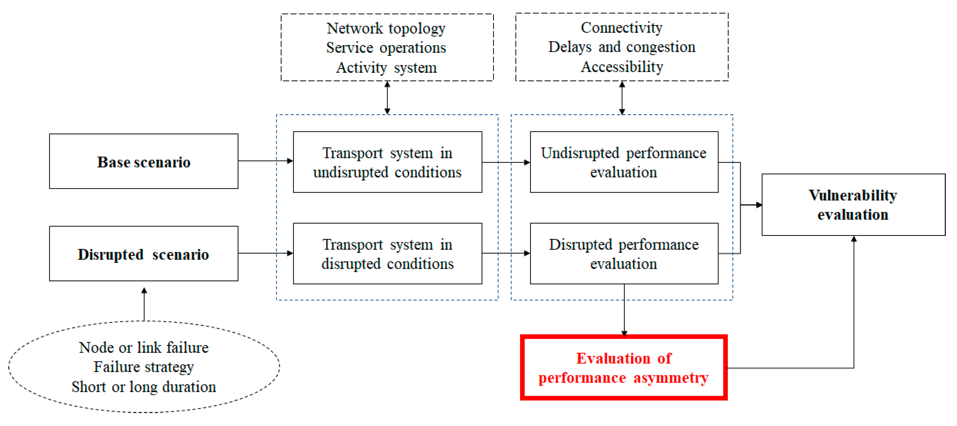
To evaluate public transport vulnerability, the common approach is to compare “base” and “disrupted” scenarios on the basis of performance indicators computed in undisrupted and degraded conditions (see Figure 1, boxes in black). The public transport network under normal operating conditions is described in the base scenario—also referred to as baseline or nominal scenario—while disrupted scenarios refer to full or partial failure of some elements of the network for a given period. Vulnerability is then measured as the change in a number of selected indicators, and the criticality of the disrupted elements is measured by performance indicators [7]. Network disruptions include node and links failure, which could be random or chosen by some pre-determined strategies [53]. Some centrality criteria are used to select potentially critical elements—whose failure is likely to cause major consequences—including current traffic loads [20,54] and probability of use [42]. Potentially critical elements may be identified also by benefitting from expert judgement without computing specific centrality measures for the network links [15,55]. However, despite reducing computational efforts, this approach may miss potentially critical locations and may then be inaccurate [16].
Here, the serviceability approach is used to define vulnerability; in particular, public transport operational degradation in the aftermath of a disruption is considered. To simulate disrupted scenarios, potentially critical links are chosen among the most central ones, which are those whose failure would cause higher impacts on the system. Link centrality is identified based on travelers’ flow in baseline operating conditions, and impacts are defined from a traveler’s perspective by evaluating passengers’ delays. The probability of occurrence of a disruption is neglected, in line with previous works [31,56]. In fact, even if some authors highlight that vulnerability derives from the combination of the probability of occurrence of a disruptive event and its consequences on the system [57,58], vulnerability has often been considered only in terms of consequences on transport system functioning, since the probability of occurrence of disruptive events is generally difficult or even impossible to determine [4].
A simulation-based approach is used here, in which the public transport system is modelled as a dynamic, stochastic system resulting from the interaction of the transport supply (network configuration and services) and transport demand sub-systems, in line with the ones proposed in [17,59,60,61,62]. The simulation model allows considering the effects of congestion and spill-over on public transportation operations, showing how flows evolve as a consequence of service or network changes, and quantifying the related effects generated on users.
Unlike existing studies on vulnerability, this study explicitly considers the distribution of impacts on travelers, particularly how delays are distributed among passengers (red box in Figure 1), in order to provide a more comprehensive representation of the consequences of vulnerability.
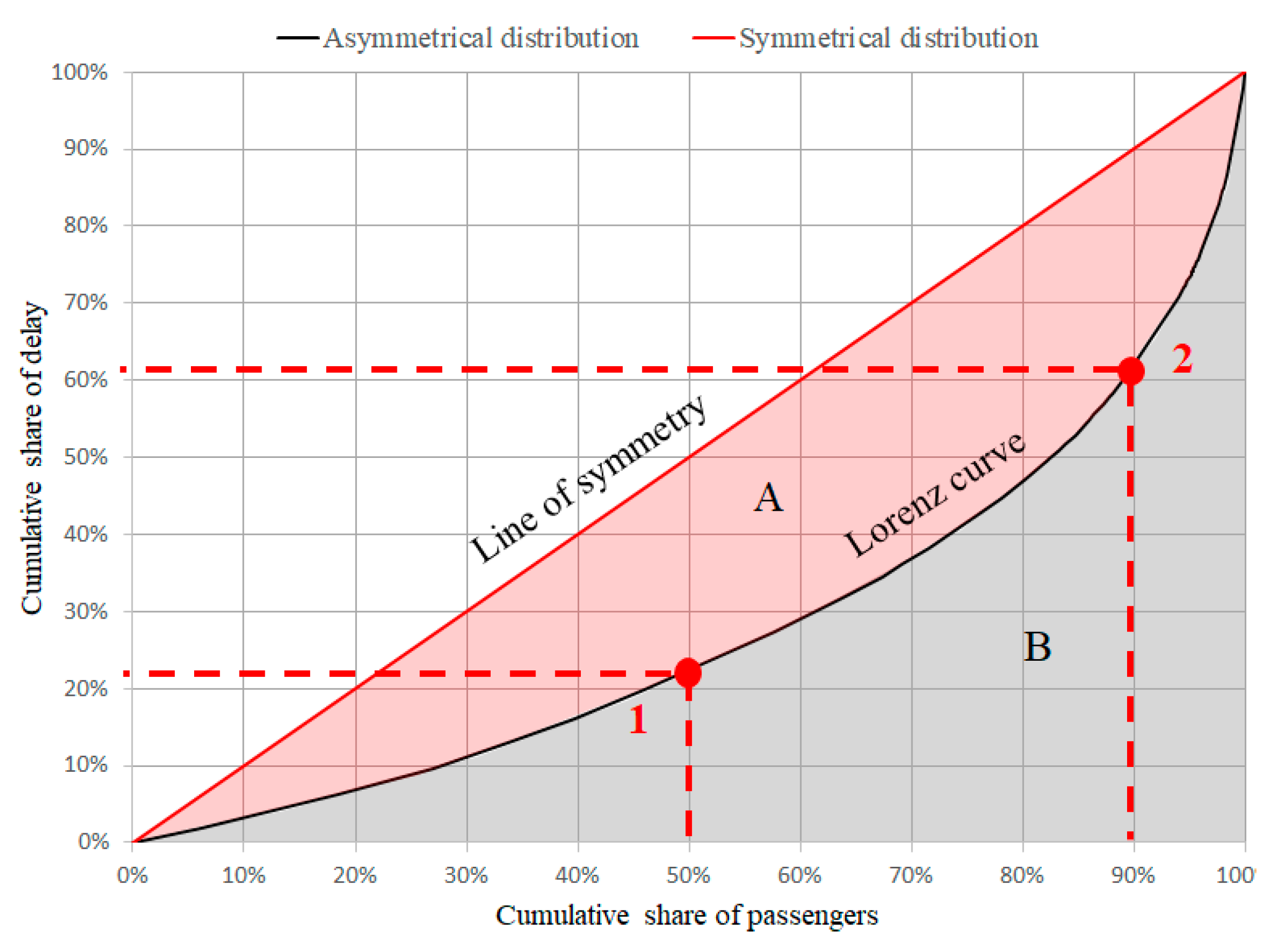
More specifically, Lorenz curves and the Gini index are used to investigate and quantify the asymmetry of disruption effects in a public transportation network. Generally speaking, the Lorenz curve depicts how a given “interest variable” is distributed among a population and is represented as a function of the cumulative proportion of the population (x-axis) and the cumulative distribution of the interest variable itself (y-axis), both quantities being represented as percentages. Here, the interest variable is the loss of public transport serviceability expressed in terms of passengers’ delay. Figure 2 shows an example of Lorenz curve representing the distribution of delays among passengers after a disruption. If the cumulative share of delays is perfectly aligned with the cumulative share of the population, the Lorenz curve results in a 45-degree straight line, known as the “line of symmetry” (in red), which represents the ideal situation of perfectly symmetrical delay distribution. On the contrary, the black curve represents an asymmetrical distribution of delays (e.g., 50% of passengers experience about 20% of the overall delay, point 1 in Figure 2).
While the Lorenz curve is useful for a graphic representation of asymmetrical distributions of delays, the Gini coefficient is a quantitative measure of the overall degree of asymmetry measured as the discrepancy between the Lorenz curve and the situation of perfectly symmetrical distribution. The Gini index is defined as the ratio of the area between the Lorenz curve and the line of symmetry (area A, red-colored in Figure 2) to the total area below the line of symmetry (area A+ area B, the latter being grey-colored in Figure 2). The value of the Gini index ranges in [0, 1]. The lower bound refers to a situation of perfect symmetry, in which the delay is the same for all passengers. When the effects of disruptions are not symmetrically distributed among passengers, the Gini index value increases as asymmetry increases.
3. Model
3.1. Public Transport System Model
The public transport service network is described by a directed graph G composed of (i) a set of nodes s (stops) representing locations where passengers can board and/or alight from public transport; (ii) a set of road links e (in the following called “line links”) representing physical connections between stops, where each e connects two adjacent stops; and (iii) a set of links g representing pedestrian links between stops [63]. A public transport line l ∊ L is defined as a sequence of line links e, L being the set of lines l. Any consecutive pair of stops (sy, sw) may be connected by: (i) a line link ely,w if a line service l exists between these two stops; (ii) a pedestrian link gy,w, otherwise. The capacity ce of the road link e is defined as the maximum number of vehicles that can use e in the time period τ (veh/τ). Finally, the transport service is realized by vehicles characterized by seat capacity and operating speed.
Travel demand SOD is modelled as a time-dependent origin-destination (OD) matrix at stop level, where each element dod represents the flow of travelers starting their trip at stop o and arriving at stop d in a given time period. For each o-d pair, a passenger n uses a path kn from the set of all the available paths Kod, kn ∊ Kod, where kn is defined as a sequence of links e. Each path may include one or more transfers, transk, occurring when two consecutive links e of kn belong to different lines.
The probability that passenger n will use path kn, pn (kn), is modelled by a multinomial logit model [63]:
where is the utility of path kn for passenger n defined as [17]
In Equation (2), is the expected waiting time at stops (both origin and transfer stops, if applicable) for passenger n; is the expected in-vehicle time on path kn, which includes running times on links and dwell times at stops; is the expected walking time on pedestrian links; is the monetary cost of kn; and is the number of transfers along kn. βs are the respective parameters. In-vehicle times are the same for passengers following the same path between o and d, while monetary costs may depend on fare policies (e.g., discounts for elderly or teenagers/children, special fares for regular working commuters, agreements with firms for discounts to their employees, etc.). Walking times depend on walking speed, which may vary among passengers following the same path. Finally, for a given o-d pair, the number of transfers may depend on the user’s choices if several alternative lines share some stops.
3.2. Simulation Model
The supply and demand models have been implemented by using BusMezzo [64,65], a mesoscopic agent-based simulator that has been previously used in the context of transit disruptions [17,35]. In BusMezzo, passengers’ decisions and transit vehicle operations are modelled at a microscopic level of detail, while traffic dynamics are represented on a mesoscopic scale. Mesoscopic simulation models allow transit dynamics to be captured even on large-scale transit networks, as vehicles are represented individually but without modelling their second-by-second movement [65,66]. As an agent-based simulator, BusMezzo models individual passengers undertaking successive adaptive decisions and is able to represent the dynamic nature of the public transport supply, including various sources of uncertainty [67]. Compared to other types of transit simulators, BusMezzo enables simulating the interaction between public transport operations and travelers’ choices, including the opportunity to switch their route after supply changes [68], different from schedule-based simulators in which passenger demand is represented as aggregate flows (e.g., VISUM). Furthermore, BusMezzo is completely integrated into the mesoscopic traffic simulation model Mezzo [63] and differs from other available agent-based transit assignment simulators (such as MATSim or MILATRAS) for the level of integration with road traffic simulation.
For each line l, scheduled vehicles realize trips between terminal stops according to the scheduled timetable. For each link e of line l, the vehicle travel time is the sum of running times on links and dwell times at stops, both described as stochastic variables. Dwell times are functions of the number of alighting and boarding passengers and depend on the type of stop (in-lane or bay) [64].
To represent day-to-day fluctuations, the number of passengers has been modelled by assuming a random Poisson process with average arrival rates corresponding to the elements of the OD matrix SOD.
The goal of each traveler n is to reach his/her trip destination at the minimum perceived generalized cost [69,70]. The progress of individual passengers is modelled as a sequence of travel decisions which are formulated as discrete random choices at certain decision times. More specifically, for each local choice (for example, boarding vs. waiting at the stop), the passenger evaluates alternatives by assessing the expected utility to arrive at its destination, conditional on taking the successive link. At a given time t’, the path is chosen on the basis of the value assumed by the variables of the utility function :
Passengers’ choices will vary according to variations in waiting and travel times, as well as vehicle capacity constraints. Utility is computed in different periods t’: (i) when the traveler starts travelling, (ii) at stops when a vehicle arrives and the traveler decides whether to board or not, and, (iii) when on board, when the traveler decides where to alight.
During the simulation, on-vehicle passenger load is recorded to identify the remaining number of passengers that can board, with the condition of seat capacity constraints. Outputs from the simulation include time-dependent statistics at passenger and stop levels, such as passengers’ travel times, vehicle loads, late vehicle arrivals at stops, number of boarding and alighting passengers, and travel times between stops.
3.3. Disrupted Scenario and Vulnerability Evaluation
Central links are identified as those intercepting as much passenger flow as possible in normal operating conditions. The centrality measure of link e, LCe, is defined as
where are the elements of the link-path incidence matrix
where kn is the path chosen by passenger n.
A disrupted scenario, δ is defined as the network state in which a disruption affects one or more links e. The disruption is modelled as a decrease in the link capacity ce for a given period tδ, ceδ being the capacity of link e in disrupted conditions, which is lower than the capacity ceb in baseline conditions. Reduction in link capacity generally causes travel time increase and then delays at successive stops with cascading effects on vehicle scheduling and waiting times at stops, which are likely to be longer. Then, passenger travel times in disrupted scenarios are generally higher than travel times in baseline conditions.
A passenger n is said to be delayed if his/her total travel time in the disrupted condition, TTnδ, is higher than his/her travel time in the baseline condition, TTnb. For a given scenario—included the baseline one—the total travel time for passenger n from o to d is given by the sum of waiting time at stops , in-vehicle times , and walking times on pedestrian links . Delay of passenger n in the disrupted scenario δ is computed as
and the average delay on the network is given by
where Nδ is the number of passengers experiencing a delay in scenario δ. The higher the average delay, the higher the vulnerability of the network in the disrupted scenario.
Once passengers’ delays are known, Lorenz curves are depicted to understand if delays are distributed symmetrically or asymmetrically among passengers. For each disrupted scenario δ, a Lorenz curve LOδ is built by evaluating the share of delay DELnδ for each delayed traveler n. Each point in the curve is identified by the set of coordinates (Xnδ; Ynδ) where Xnδ is the cumulated proportion of passengers (Xnδ< Xn+1δ) and Ynδ is the corresponding cumulated proportion of delays. Finally, the Gini index in scenario δ, is computed as
where X0δ = Y0 = 0, Xnδδ = Ynδ = 1, and VGINIδ ranges in [0, 1].
4. Case Study
4.1. Public Transport System Description and Implementation
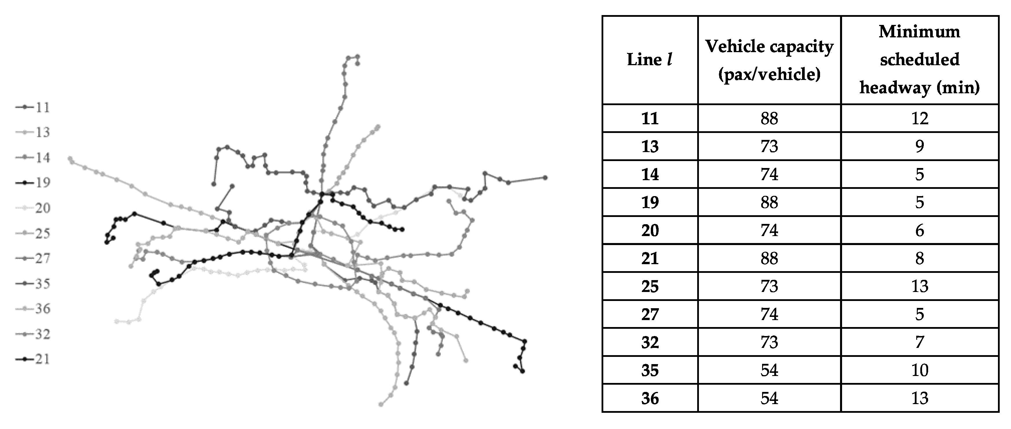
The proposed approach has been applied to the case study of Bologna, a mid-sized city (around 380,000 inhabitants) in Northern Italy. Its public transport network, shown in Figure 3, consists of 11 bus lines (in both directions), with 659 nodes (stops) and 770 links. Lines are operated by vehicles having different values of seat capacity and are characterized by maximum scheduled frequency and operating speeds. Key attributes of each line are also provided in Figure 3. The coordinates of each stop, vehicle characteristics and line timetables have been obtained from available open data (https://www.tper.it/tper-open-data) (accessed on 1 August 2021).
Utility function coefficients in Equation (2) have not been calibrated for the case study; however, proper values can be found in the literature which are appropriate for the socio-economic context of the study area. In particular, the values estimated in [71] have been assumed suitable for this case: βwait = βg = −0.07, βivt = −0.04, and βtrans = −0.334. As for monetary costs, in the case study, the ticket fare is the same for all the lines, and then for all paths, i.e., no single ticket discounts for users’ categories exist, and fare zones are not applied so that the hypothesis that the user’s path choices are not affected by monetary costs is reasonable. In the considered case study, information regarding expected remaining time until next vehicle arrival for all lines serving all connected stops is provided to passengers at stops. Finally, when using connection links between stops, passengers are assumed to walk at a constant speed vg = 1.2 m/s (~4.5 km/h) with a maximum walking threshold of 500 m.
As other similar cities, the Bologna public transport service has experimented disruptions such as vehicle breakdowns, infrastructure issues, accidents, and floods. In the several scenarios, the public transport supply is simulated starting at 7:00 a.m. until 12:00 a.m. (T = 5 h) in order to be realistic with operating conditions—i.e., the service starts according to scheduled timetable, while transport demand will use the service according to its specific needs. As the most interesting condition occurs during peak hours, the passenger demand refers to the peak morning period 7:30–9:30 a.m. Passenger demand data, collected during an on-board survey campaign in 2018, have been provided by the transit service operator and refer to passenger trips during a weekday morning peak-period between 7:30 and 9:30 a.m. In the first half hour, from 7:00 to 7:30 a.m., the simulation allows positioning the vehicles in the network according to the planned schedule in order to ensure that when peak-hours passengers start their journey at 7:30 a.m., the service is available at all locations. The remaining period until 12:00 a.m. allows simulating how the peak-hours demand is affected by disruptions and how these effects are distributed among passengers. The time length T has been considered suitable to let passengers complete their journey according to the nature of the disruption.
During T, 10 simulations have been considered, which leads to a maximum error less than 5% for estimating the passenger travel time. To validate the model, simulated bus travel times and passenger loads throughout the network in undisrupted conditions are compared with data collected and made available by the service operator, including average travel times and loads.
4.2. Disrupted Scenario Definition: Central Links Identification
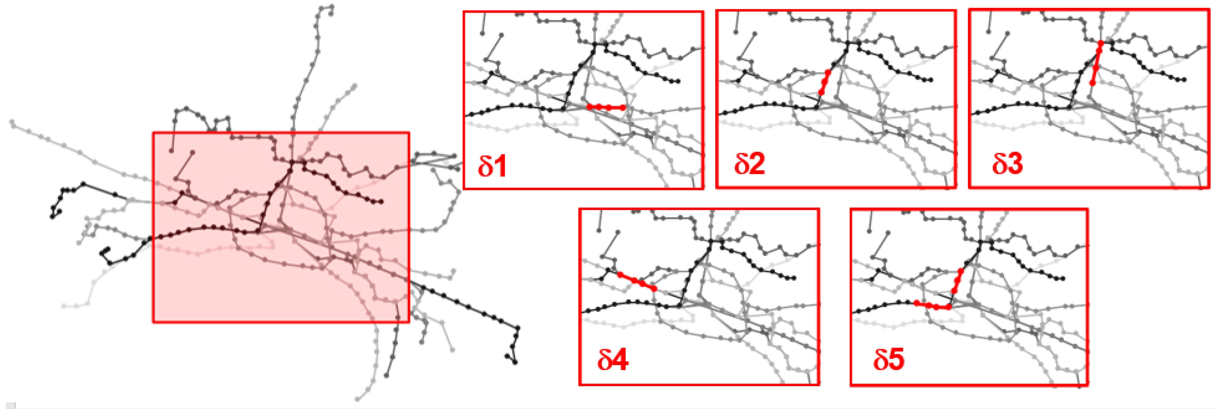
The load centrality LCe of each link has been computed in the baseline scenario, and links have been ranked according to it. The first five links have been selected for modelling five disrupted scenarios δ. More specifically, the first scenario corresponds to the disruption of the first-ranked link, the second to the second-ranked, and so on. In addition, for a more realistic representation, adjacent links to the most central ones having similar LCe values (up to 10% difference) have also been disrupted to assure line closures of a relevant length—which have been identified as “segment”. Table 1 and Figure 4 show the links with the highest LCe values that were selected for modelling the disrupted Scenarios (δ1–δ5). The simulated disruption corresponds to the complete closure of the segment due to unexpected events (such as road accidents or infrastructure issues), and then the capacity ce of such links has been set to zero for the morning peak-hour between 8:00 and 9:00 a.m. (tδ= 1 h). Moreover, no service replacement has been planned, due to both the unexpected nature of the event and the short duration of the disruption. For such scenarios, vulnerability has been quantified in terms of average passenger delays (see Section 3, Equations (6) and (7)). Then, the Lorenz curves LOδ1−5 and Gini indices VGINIδ1–5 have been computed, in order to refine the evaluation of the disruption impacts according to the proposed approach.
5. Results and Discussion
Transport system performance is evaluated for the simulation period 7:00–12:00 a.m., with a transport demand of almost 50,000 travelers. The system operating conditions for the baseline scenario (also referred to as b) are assumed to be ideal and to proceed as scheduled; in this situation, passengers do not experience any delay, and the average simulated travel time (consisting of waiting, in-vehicle, and walking times) is 34 min. Half of passengers take between 5 and 25 min to complete their paths.
Table 2 shows the average simulated travel times in the base (b) and disrupted Scenarios (δ1–δ5). As can be seen, the average travel time remains almost the same among the considered scenarios, with just a slight difference (about 3 min at most). The average travel time is not able to capture the effects of a disrupted network condition, particularly for verifying the impacts produced on the users that are mainly affected by disruptions. In order to have a clearer view of such effects, the number of passengers who experience a delay should be explicitly considered, and delay distribution among such passengers should be computed.
As reported in Table 2, the percentage of passengers suffering from a delay varies in the five scenarios between 11% (the lowest, in δ3) and 20% (the highest, in δ2), while the average passengers’ delay is computed as in Equation (7) by taking into account only delayed passengers. The average delays for delayed passengers range between 12 and 17 min, as shown in Figure 5a (standard deviation of is also reported). The scenarios with the highest average delay are δ1 and δ2, with average delays of 16 and 17 min, respectively. However, the delay varies significantly among travelers, depending on the origin-destination pair and path choice (see Figure 5b). In particular, some passengers experience more than 1 h delay, especially in δ1 (3.4%) and δ2 (4.0%). For these passengers, the disrupted segments play a relevant role in connecting their o-d, since no other acceptable alternatives are available.
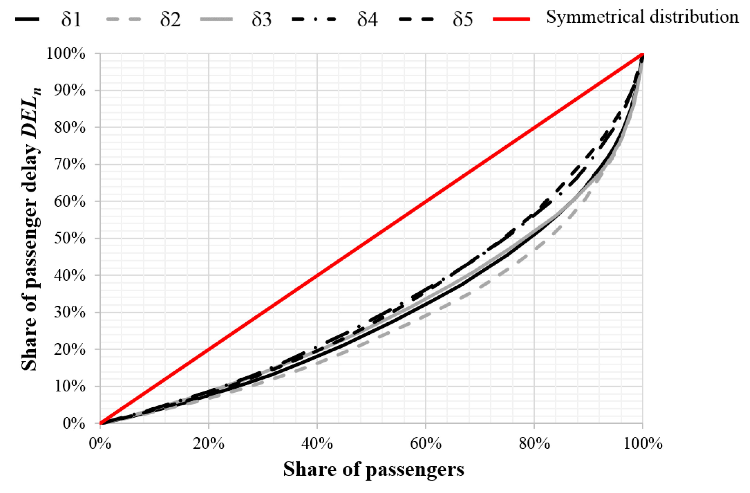
To identify the (a) symmetry of impacts, the Lorenz curves LOδ are depicted in Figure 6 for the five scenarios, while the Gini coefficients VGINIδ are provided in Table 3. Overall, the curves suggest relatively low symmetry in terms of impacts on passengers, as showed by the difference between the symmetrical distribution line (in red in Figure 6) and the Lorenz curves, and only a small fraction of users experiences the majority of delays. Similarly, the Gini indices VGINIδ vary in the five scenarios ranging from 0.34 to 0.44, confirming that delay distributions are far from perfectly symmetrical.
The most asymmetrical scenario is δ2 (VGINIδ = 0.44), with passengers experiencing delays also greater than 1 h. In this scenario, 80% of delayed passengers experience only 45% of the total amount of delay, while the remaining 20% of passengers experience the majority of delays. Referring to cases δ1 and δ3, delays are slightly more symmetrical: in these cases, 80% of the passengers share approximately 50% of delays. Scenarios δ4 and δ5, in which the disrupted links are the less central ones among the considered cases, have similar and lower Gini indices (VGINIδ = 0.34), suggesting a slightly more symmetric delay distribution.
As shown by the simulation results, the links with higher centrality LCe are generally the ones whose closure causes the highest average delay (see Table 3). In the scenarios where the most central links are closed (δ1 and δ2), the magnitude of the impact is greater, and the network is more vulnerable. Conversely, for Scenarios δ3 and δ5, delays are lower and the network less vulnerable. These results seem to suggest the existence of some correlation between the centrality measure and the network vulnerability, although the centrality of a link does not necessarily mean that its closure leads to the most critical situation, particularly in terms of asymmetry of impacts (compare, for example, Scenarios δ1 and δ2 in Table 3).
Evaluating disrupted performance only in terms of aggregate network indicators—such as the average travel times or average delays—may not be enough for an in-depth understanding of vulnerability. The use of Lorenz curves and the Gini index characterizes the vulnerability of the disrupted system with more details. In particular, the obtained results show that Scenarios δ1 and δ2, where disrupted links are the most central ones, also have higher Gini indices. In such cases, delays are asymmetrically distributed and concentrated on few passengers, whose experienced impacts are higher than those expressed by the average delay indicator. More specifically, by considering only average delays, scenario δ5 ( = 14.51 min) would be comparable to scenario δ1 ( = 15.74 min). Nevertheless, Lorenz curves show that delays are more symmetrically distributed among passengers in δ5 than in δ1 (VGINIδ5 = 0.344 vs. VGINIδ1 = 0.402), with δ5 being less vulnerable than δ1. Even if average delays are similar, the disrupted conditions of the system in the two cases are not the same, as delays distribute differently, as do the effects perceived by users.
The additional computation of the Gini index contributes to a better understanding of public transport system vulnerability, by combining network level (delays) and concentration (Gini index) indicators.
The proposed methodology may help transport system planners and operators to identify vulnerable scenarios together with links that should be prioritized when planning maintenance, emergency, and actions (such as providing alternative routes or vehicles or upgrading existing service or infrastructure). Furthermore, the estimate of asymmetries can support the implementation of public transportation equity policies in order to highlight any potentially disadvantaged class of users in terms of accessibility and disruption effects. Particularly, the combined use of average delays, Lorenz curves, and the Gini index may help stakeholders to define thresholds for the acceptability of imbalance in the distribution of delays and to set up actions for compensation.
6. Conclusions and Further Research
This paper presents a new approach to analyze the vulnerability of public transport systems that is based on the combination of network indicators and impact (a) symmetry evaluation. To the authors’ knowledge, this approach has not yet been considered in the transport vulnerability literature and practice, as previous studies generally deal with vulnerability in terms of network-level indicators such as average delay or increased generalized cost. The methodological framework proposed in this work relies on classical approaches by using the Lorenz curve and Gini index to analyze delay symmetry on travelers and identify delay imbalances among passengers.
The enrichment of vulnerability analysis by means of the inclusion of delay asymmetry evaluation allows computing better public transport system performances in the case of disruption. By considering both these elements, operators and planners of public transport systems are provided with a better understanding of how the effects of a disruption affect users. This, along with the identification of critical locations, is also of utmost importance for devising measures and strategies to safeguard network performance, for allocating maintenance or emergency resources, and for supporting the implementation of policies aimed at public transportation equity.
The analysis performed on a public transport network of a medium-sized city showed that, in general, average user travel time is not sufficient to compare network performance under normal and disrupted conditions. On the contrary, quantifying the delay experienced by users under disrupted conditions and the asymmetry of its distribution may have important impacts on setting up equity policies. The results for the test case showed that some of the tested scenarios, while showing similar results in terms of vulnerability from the point of view of average delays, actually involve differences in terms of the distribution of impacts among users.
Further research is expected in terms of different performance measures that could be used to determine public transport vulnerability by suitably weighting several components of the total travel times, such as increased walking times and additional transfers in the re-routed path, as well as the effects of on-board crowding on perceived level of service. In addition, Lorenz curve-based vulnerability analysis may be applied to different transport modes, such as individual road transport or air transport, by using suitable performance measures.
Author Contributions
Conceptualization, C.M., L.M., F.P. and M.N.P.; methodology, C.M., L.M., F.P. and M.N.P.; validation, C.M., L.M., F.P. and M.N.P.; data curation, C.M., L.M., F.P. and M.N.P.; writing—original draft preparation, C.M., L.M., F.P. and M.N.P.; writing—review and editing, C.M., L.M., F.P. and M.N.P.; supervision, C.M., L.M., F.P. and M.N.P. All authors have read and agreed to the published version of the manuscript.
Funding
This research received no external funding.
Data Availability Statement
Data used to model the analyzed public transport system have been obtained from open data made available by the public service provider (https://www.tper.it/tper-open-data) (accessed on 1 August 2021).
Conflicts of Interest
The authors declare no conflict of interest.
References
- Saxena, N.; Rashidi, T.H.; Auld, J. Studying the tastes effecting mode choice behavior of travelers under transit service disruptions. Travel Behav. Soc. 2019, 17, 86–95. [Google Scholar] [CrossRef]
- Xia, T.; Nitschke, M.; Zhang, Y.; Shah, P.; Crabb, S.; Hansen, A. Traffic-related air pollution and health co-benefits of alternative transport in Adelaide, South Australia. Environ. Int. 2015, 74, 281–290. [Google Scholar] [CrossRef]
- Moniruzzaman, M.; Páez, A. Accessibility to transit, by transit, and mode share: Application of a logistic model with spatial filters. J. Transp. Geogr. 2012, 24, 198–205. [Google Scholar] [CrossRef]
- Gu, Y.; Fu, X.; Liu, Z.; Xu, X.; Chen, A. Performance of transportation network under perturbations: Reliability, vulnerability, and resilience. Transp. Res. Part E Logis. Transp. Rev. 2020, 133, 101809. [Google Scholar] [CrossRef]
- Li, T.; Rong, L.; Yan, K. Vulnerability analysis and critical area identification of public transport system: A case of high-speed rail and air transport coupling system in China. Transp. Res. Part A Policy Pract. 2019, 127, 55–70. [Google Scholar] [CrossRef]
- Zhu, S.; Levinson, D.M. Disruptions to transportation networks: A review. In Network Reliability in Practice; Levinson, D.M., Liu, H.X., Bell, M., Eds.; Springer: New York, NY, USA, 2012; pp. 5–20. [Google Scholar]
- de Oliveira, E.L.; da Silva Portugal, L.; Junior, W.P. Indicators of reliability and vulnerability: Similarities and differences in ranking links of a complex road system. Transp. Res. Part A Policy Pract. 2016, 88, 195–208. [Google Scholar] [CrossRef]
- Lu, Q.C.; Lin, S. Vulnerability analysis of urban rail transit network within multi-modal public transport networks. Sustainability 2019, 11, 2109. [Google Scholar] [CrossRef] [Green Version]
- Rodríguez-Núñez, E.; García-Palomares, J.C. Measuring the vulnerability of public transport networks. J. Transp. Geogr. 2014, 35, 50–63. [Google Scholar] [CrossRef] [Green Version]
- Yap, M.; Cats, O. Predicting disruptions and their passenger delay impacts for public transport stops. Transportation 2020, 48, 1703–1731. [Google Scholar] [CrossRef]
- Hörcher, D.; Graham, D.J.; Anderson, R.J. Crowding cost estimation with large scale smart card and vehicle location data. Transp. Res. Part B Meth. 2017, 95, 105–125. [Google Scholar] [CrossRef]
- Yap, M.D.; van Oort, N.; van Nes, R.; van Arem, B. Identification and quantification of link vulnerability in multi-level public transport networks: A passenger perspective. Transportation 2018, 45, 1161–1180. [Google Scholar] [CrossRef] [Green Version]
- Chen, A.; Yang, C.; Kongsomsaksakul, S.; Lee, M. Network-based accessibility measures for vulnerability analysis of degradable transportation networks. Netw. Spat. Econ. 2007, 7, 241–256. [Google Scholar] [CrossRef]
- Adelé, S.; Tréfond-Alexandre, S.; Dionisio, C.; Hoyau, P.A. Exploring the behavior of suburban train users in the event of disruptions. Transp. Res. Part F Traffic Psychol. Behav. 2019, 65, 344–362. [Google Scholar] [CrossRef]
- Taylor, M.A.P.; Susilawati, S. Remoteness and accessibility in the vulnerability analysis of regional road networks. Transp. Res. Part A Policy Pract. 2012, 46, 761–771. [Google Scholar] [CrossRef]
- Taylor, M. Vulnerability Analysis for Transportation Networks; Elsevier: Amsterdam, The Netherlands, 2017. [Google Scholar]
- Cats, O.; Jenelius, E. Dynamic vulnerability analysis of public transport networks: Mitigation effects of real-time information. Netw. Spat. Econ. 2014, 14, 435–463. [Google Scholar] [CrossRef]
- Zhang, J.; Hu, F.; Wang, S.; Dai, Y.; Wang, Y. Structural vulnerability and intervention of high speed railway networks. Phys. A Stat. Mech. Appl. 2016, 462, 743–751. [Google Scholar] [CrossRef]
- Zhang, J.; Wang, S.; Wang, X. Comparison analysis on vulnerability of metro networks based on complex network. Phys. A Stat. Mech. Appl. 2018, 496, 72–78. [Google Scholar] [CrossRef]
- Jenelius, E. Network structure and travel patterns: Explaining the geographical disparities of road network vulnerability. J. Transp. Geogr. 2009, 17, 234–244. [Google Scholar] [CrossRef]
- Mishra, S.; Welch, T.F.; Jha, M.K. Performance indicators for public transit connectivity in multi-modal transportation networks. Transp. Res. Part A Policy Pract. 2012, 46, 1066–1085. [Google Scholar] [CrossRef]
- Sun, D.J.; Zhao, Y.; Lu, Q.C. Vulnerability analysis of urban rail transit networks: A case study of Shanghai, China. Sustainability 2015, 7, 6919–6936. [Google Scholar] [CrossRef] [Green Version]
- Latora, V.; Marchiori, M. Efficient behavior of small-world networks. Phys. Rev. Lett. 2001, 87, 198701. [Google Scholar] [CrossRef] [PubMed] [Green Version]
- Vragović, I.; Louis, E.; Díaz-Guilera, A. Efficiency of informational transfer in regular and complex networks. Phys. Rev. E 2005, 71, 036122. [Google Scholar] [CrossRef] [Green Version]
- Shi, J.; Wen, S.; Zhao, X.; Wu, G. Sustainable development of urban rail transit networks: A vulnerability perspective. Sustainability 2019, 11, 1335. [Google Scholar] [CrossRef] [Green Version]
- Duan, Y.; Lu, F. Robustness of city road networks at different granularities. Phys. A Stat. Mech. Appl. 2014, 411, 21–34. [Google Scholar] [CrossRef]
- Zhang, X.; Miller-Hooks, E.; Denny, K. Assessing the role of network topology in transportation network resilience. J. Transp. Geogr. 2015, 46, 35–45. [Google Scholar] [CrossRef] [Green Version]
- Balijepalli, C.; Oppong, O. Measuring vulnerability of road network considering the extent of serviceability of critical road links in urban areas. J. Transp. Geogr. 2014, 39, 145–155. [Google Scholar] [CrossRef]
- Cats, O.; Jenelius, E. Beyond a complete failure: The impact of partial capacity degradation on public transport network vulnerability. Transp. B Transp. Dyn. 2018, 6, 77–96. [Google Scholar] [CrossRef] [Green Version]
- Leng, J.Q.; Zhai, J.; Li, Q.W.; Zhao, L. Construction of road network vulnerability evaluation index based on general travel cost. Phys. A Stat. Mech. Appl. 2018, 493, 421–429. [Google Scholar] [CrossRef]
- Jenelius, E.; Mattsson, L.G. Road network vulnerability analysis of area-covering disruptions: A grid-based approach with case study. Transp. Res. Part A Policy Pract. 2012, 46, 746–760. [Google Scholar] [CrossRef]
- Scott, D.M.; Novak, D.C.; Aultman-Hall, L.; Guo, F. Network robustness index: A new method for identifying critical links and evaluating the performance of transportation networks. J. Transp. Geogr. 2006, 14, 215–227. [Google Scholar] [CrossRef]
- Sullivan, J.L.; Novak, D.C.; Aultman-Hall, L.; Scott, D.M. Identifying critical road segments and measuring system-wide robustness in transportation networks with isolating links: A link-based capacity-reduction approach. Transp. Res. Part A Policy Pract. 2010, 44, 323–336. [Google Scholar] [CrossRef]
- Leng, N.; Corman, F. The role of information availability to passengers in public transport disruptions: An agent-based simulation approach. Transp. Res. Part A Policy Pract. 2020, 133, 214–236. [Google Scholar] [CrossRef]
- Malandri, C.; Fonzone, A.; Cats, O. Recovery time and propagation effects of passenger transport disruptions. Phys. A Stat. Mech. Appl. 2018, 505, 7–17. [Google Scholar] [CrossRef] [Green Version]
- Snelder, M.; Calvert, S. Quantifying the impact of adverse weather conditions on road network performance. Eur. J. Transp. Infrastruct. Res. 2016, 16, 3118. [Google Scholar]
- Dehghani, M.S.; Flintsch, G.; McNeil, S. Impact of road conditions and disruption uncertainties on network vulnerability. J. Infrastruct. Syst. 2014, 20, 04014015. [Google Scholar] [CrossRef]
- Murray-Tuite, P.M.; Mahmassani, H.S. Methodology for determining vulnerable links in a transportation network. Transp. Res. Rec. 2004, 1882, 88–96. [Google Scholar] [CrossRef]
- Connors, R.D.; Watling, D.P. Assessing the demand vulnerability of equilibrium traffic networks via network aggregation. Netw. Spat. Econ. 2015, 15, 367–395. [Google Scholar] [CrossRef] [Green Version]
- Chen, B.Y.; Lam, W.H.; Sumalee, A.; Li, Q.; Li, Z.C. Vulnerability analysis for large-scale and congested road networks with demand uncertainty. Transp. Res. Part A Policy Pract. 2012, 46, 501–516. [Google Scholar] [CrossRef]
- Taylor, M.; Sekhar, S.; D’Este, G. Application of accessibility based methods for vulnerability analysis of strategic road networks. Netw. Spat. Econ. 2006, 6, 267–291. [Google Scholar] [CrossRef]
- D’este, G.A.; Taylor, M.A. Network Vulnerability: An Approach to Reliability Analysis at the Level of National Strategic Transport Networks; Emerald Group Publishing Limited: Bingley, UK, 2003. [Google Scholar]
- Taylor, M.A.; D’Este, G.M. Transport network vulnerability: A method for diagnosis of critical locations in transport infrastructure systems. In Critical Infrastructure; Springer: Berlin/Heidelberg, Germany, 2007; pp. 9–30. [Google Scholar]
- Lorenz, M.O. Methods of measuring the concentration of wealth. Publ. Am. Stat. Assoc. 1905, 9, 209–219. [Google Scholar] [CrossRef]
- Delbosc, A.; Currie, G. Using Lorenz curves to assess public transport equity. J. Transp. Geogr. 2011, 19, 1252–1259. [Google Scholar] [CrossRef]
- Jang, S.; An, Y.; Yi, C.; Lee, S. Assessing the spatial equity of Seoul’s public transportation using the Gini coefficient based on its accessibility. Int. J. Urban Sci. 2017, 21, 91–107. [Google Scholar] [CrossRef]
- Lope, D.J.; Dolgun, A. Measuring the inequality of accessible trams in Melbourne. J. Transp. Geogr. 2020, 83, 102657. [Google Scholar] [CrossRef]
- Gallo, M. Assessing the equality of external benefits in public transport investments: The impact of urban railways on real estate values. Case Stud. Transp. Policy 2020, 8, 758–769. [Google Scholar] [CrossRef]
- Guzman, L.A.; Oviedo, D.; Rivera, C. Assessing equity in transport accessibility to work and study: The Bogotá region. J. Transp. Geogr. 2017, 58, 236–246. [Google Scholar] [CrossRef]
- Chen, Y.; Bouferguene, A.; Li, H.X.; Liu, H.; Shen, Y.; Al-Hussein, M. Spatial gaps in urban public transport supply and demand from the perspective of sustainability. J. Clean. Prod. 2018, 195, 1237–1248. [Google Scholar] [CrossRef]
- Pavkova, K.; Currie, G.; Delbosc, A.; Sarvi, M. Selecting tram links for priority treatments-The Lorenz Curve approach. J. Transp. Geogr. 2016, 55, 101–109. [Google Scholar] [CrossRef]
- Hörcher, D.; Graham, D.J. The Gini Index of Demand Imbalances in Public Transport; Springer: Berlin/Heidelberg, Germany, 2020; pp. 1–24. [Google Scholar] [CrossRef]
- Berche, B.; Von Ferber, C.; Holovatch, T.; Holovatch, Y. Resilience of public transport networks against attacks. Eur. Phys. J. B 2009, 71, 125–137. [Google Scholar] [CrossRef] [Green Version]
- Sun, D.J.; Guan, S. Measuring vulnerability of urban metro network from line operation perspective. Transp. Res. Part A Policy Pract. 2016, 94, 348–359. [Google Scholar] [CrossRef]
- Peterson, S.K.; Church, R.L. A framework for modeling rail transport vulnerability. Growth Chang. 2008, 39, 617–641. [Google Scholar] [CrossRef]
- Faturechi, R.; Miller-Hooks, E. Measuring the performance of transportation infrastructure systems in disasters: A comprehensive review. J. Infrastruct. Syst. 2015, 21, 04014025. [Google Scholar] [CrossRef]
- Jenelius, E.; Petersen, T.; Mattsson, L.G. Importance and exposure in road network vulnerability analysis. Transp. Res. Part A Policy Pract. 2006, 40, 537–560. [Google Scholar] [CrossRef]
- Wang, Z.; Chan, A.P.; Yuan, J.; Xia, B.; Skitmore, M.; Li, Q. Recent advances in modeling the vulnerability of transportation networks. J. Infrastruct. Syst. 2015, 21, 06014002. [Google Scholar] [CrossRef]
- Cats, O.; Jenelius, E. Planning for the unexpected: The value of reserve capacity for public transport network robustness. Transp. Res. Part A Policy Pract. 2015, 81, 47–61. [Google Scholar] [CrossRef]
- Cats, O.; Yap, M.; Van Oort, N. Exposing the role of exposure: Public transport network risk analysis. Transp. Res. Part A Policy Pract. 2016, 88, 1–14. [Google Scholar] [CrossRef]
- Cats, O.; West, J.; Eliasson, J. A Dynamic Stochastic Model for Evaluating Congestion and Crowding Effects in Transit Systems. Transp. Res. Part B Meth. 2016, 89, 43–57. [Google Scholar] [CrossRef] [Green Version]
- Malandri, C.; Mantecchini, L.; Postorino, M.N. Airport ground access reliability and resilience of transit networks: A case study. Transp. Res. Proc. 2017, 27, 1129–1136. [Google Scholar] [CrossRef]
- Gentile, G.; Nökel, K. Modelling Public Transport Passenger Flows in the Era of Intelligent Transport Systems; Springer International Publishing: New York, NY, USA, 2016; p. 10. [Google Scholar]
- Cats, O.; Burghout, W.; Toledo, T.; Koutsopoulos, H.N. Mesoscopic Modeling of Bus Public Transportation. Transp. Res. Rec. 2010, 2188, 9–18. [Google Scholar] [CrossRef]
- Toledo, T.; Cats, O.; Burghout, W.; Koutsopoulos, H.N. Mesoscopic Simulation for Transit Operations. Transp. Res. Part C Emerg. Technol. 2010, 18, 896–908. [Google Scholar] [CrossRef] [Green Version]
- Cats, O. Multi-agent transit operations and assignment model. Procedia Comput. Sci. 2013, 19, 809–814. [Google Scholar] [CrossRef] [Green Version]
- Nuzzolo, A.; Lam, W.H. Modelling Intelligent Multi-Modal Transit Systems; CRC Press: Boca Raton, FL, USA, 2017. [Google Scholar]
- Cats, O.; Hartl, M. Modelling public transport on-board congestion: Comparing schedule-based and agent-based assignment approaches and their implications. J. Adv. Transp. 2016, 50, 1209–1224. [Google Scholar] [CrossRef] [Green Version]
- Ben-Akiva, M.; Lerman, S.R. Discrete Choice Analysis; MIT Press: Cambridge, MA, USA, 1985. [Google Scholar]
- Train, K. Discrete Choice Methods with Simulation; Cambridge University Press: Cambridge, UK, 2003. [Google Scholar]
- Cats, O.; Koutsopoulos, H.N.; Burghout, W.; Toledo, T. Effect of real-time transit information on dynamic path choice of passengers. Transp. Res. Rec. 2011, 2217, 46–54. [Google Scholar] [CrossRef] [Green Version]
Figure 1.
Procedure for evaluating transport network vulnerability.

Figure 2.
Lorenz curve to identify delay distribution.

Figure 3.
Public network characteristics of the case study.

Figure 4.
Central links and disrupted segments (highlighted in red in the five scenarios δ1–δ5).

Figure 5.
(a) Average passenger delay and (b) delay distribution among passengers for scenarios (δ1–δ5).
Figure 5.
(a) Average passenger delay and (b) delay distribution among passengers for scenarios (δ1–δ5).

Figure 6.
Lorenz curves for Scenarios (δ1–δ5).


Table 1.
Central links characteristics and centrality measure.
| Scenario | Disrupted Lines | Disrupted Segment Length (m) | LCe |
|---|---|---|---|
| δ1 | 14, 11, 13, 19, 20, 25, 27 | 900 | 25,382 |
| δ2 | 13, 19, 21, 25, 35, 36 | 1300 | 19,772 |
| δ3 | 11, 20, 21, 25 | 1300 | 19,603 |
| δ4 | 13, 19, 36 | 850 | 13,246 |
| δ5 | 14, 20, 21 | 1000 | 13,200 |
Table 2.
Average travel times and percentage of delayed passengers.
| Scenario | Average Travel Time (min) | Percentage of Delayed Passengers (%) |
|---|---|---|
| b | 34.19 | 0 |
| δ1 | 36.80 | 15.38 |
| δ2 | 37.80 | 20.22 |
| δ3 | 35.46 | 11.51 |
| δ4 | 35.28 | 18.14 |
| δ5 | 36.55 | 14.79 |
Table 3.
Vulnerability Gini indices, load centrality, and average passenger delay for Scenarios (δ1–δ5).
Table 3.
Vulnerability Gini indices, load centrality, and average passenger delay for Scenarios (δ1–δ5).
| Scenario | VGINIδ | LCe | (min) |
|---|---|---|---|
| δ1 | 0.40238 | 25,382 | 15.74 |
| δ2 | 0.44415 | 19,772 | 16.88 |
| δ3 | 0.38586 | 19,603 | 13.79 |
| δ4 | 0.34230 | 13,246 | 12.99 |
| δ5 | 0.34366 | 13,200 | 14.51 |
Publisher’s Note: MDPI stays neutral with regard to jurisdictional claims in published maps and institutional affiliations. |
© 2021 by the authors. Licensee MDPI, Basel, Switzerland. This article is an open access article distributed under the terms and conditions of the Creative Commons Attribution (CC BY) license (https://creativecommons.org/licenses/by/4.0/).
Share and Cite
MDPI and ACS Style
Malandri, C.; Mantecchini, L.; Paganelli, F.; Postorino, M.N. Public Transport Network Vulnerability and Delay Distribution among Travelers. Sustainability 2021, 13, 8737. https://0-doi-org.brum.beds.ac.uk/10.3390/su13168737
AMA Style
Malandri C, Mantecchini L, Paganelli F, Postorino MN. Public Transport Network Vulnerability and Delay Distribution among Travelers. Sustainability. 2021; 13(16):8737. https://0-doi-org.brum.beds.ac.uk/10.3390/su13168737
Chicago/Turabian StyleMalandri, Caterina, Luca Mantecchini, Filippo Paganelli, and Maria Nadia Postorino. 2021. "Public Transport Network Vulnerability and Delay Distribution among Travelers" Sustainability 13, no. 16: 8737. https://0-doi-org.brum.beds.ac.uk/10.3390/su13168737
Note that from the first issue of 2016, this journal uses article numbers instead of page numbers. See further details here.