Addressing Nutrient Depletion in Tanzanian Sisal Fiber Production Using Life Cycle Assessment and Circular Economy Principles, with Bioenergy Co-Production

Colley, Tracey Anne; Valerian, Judith; Hauschild, Michael Zwicky; Olsen, Stig Irving; Birkved, Morten

doi:10.3390/su13168881

Open AccessArticle

Addressing Nutrient Depletion in Tanzanian Sisal Fiber Production Using Life Cycle Assessment and Circular Economy Principles, with Bioenergy Co-Production

¹

Quantitative Sustainability Assessment (QSA) Group, Department of Technology, Sustainability Division, Management and Economics, Technical University of Denmark (DTU), DK-2800 Kgs. Lyngby, Denmark

²

Department of Food and Resource Economics (DeFRE), School of Agriculture Economics and Business Studies (SAEBS), Sokoine University of Agriculture (SUA), P.O. Box 3007 Morogoro, Tanzania

³

SDU Life Cycle Engineering, Institut for Grøn Teknologi (IGT), University of Southern Denmark, DK-5230 Odense, Denmark

^*

Author to whom correspondence should be addressed.

Sustainability 2021, 13(16), 8881; https://0-doi-org.brum.beds.ac.uk/10.3390/su13168881

Submission received: 9 July 2021 / Revised: 26 July 2021 / Accepted: 30 July 2021 / Published: 9 August 2021

(This article belongs to the Section Environmental Sustainability and Applications)

Download

Browse Figures

Versions Notes

Abstract

:

Nutrient depletion in Tanzanian sisal production has led to yield decreases over time. We use nutrient mass balances embedded within a life cycle assessment to quantify the extent of nutrient depletion for different production systems, and then used circular economy principles to identify potential cosubstrates from within the Tanzanian economy to anaerobically digest with sisal wastes. The biogas produced was then used to generate bioelectricity and the digestate residual can be used as a fertilizer to address the nutrient depletion. Life cycle assessment was used in a gate-to-gate assessment of the anaerobic digestion options with different cosubstrates. If no current beneficial use of the cosubstrate was assumed, then beef manure and marine fish processing waste were the best cosubstrates. If agricultural wastes were assumed to have a current beneficial use as fertilizer, then marine fish processing waste and human urine were the best cosubstrates. The largest reduction in environmental impacts resulted from bioelectricity replacing electricity from fossil fuels in the national electricity grid and improved onsite waste management practices. There is significant potential to revitalize Tanzanian sisal production by applying circular economy principles to sisal waste management to address soil nutrient depletion and co-produce bioenergy.

Keywords:

life cycle assessment; sisal production; circular economy; nutrient depletion; anaerobic digestion; waste management; bioenergy; biogas; Tanzania

1. Introduction

Sisal (Agave sisalana) was imported from Mexico’s Yucatan Peninsula into Tanzania during the late 1800s [1]. Tanzania was the world’s second-largest producer of sisal in 2019, producing 15% of the world’s 220,363 tonnes of sisal fiber [2] behind Brazil, which produced 39% of the world’s production. The three key factors that determine the export sisal fiber yield per hectare are: the mass of sisal leaves produced per hectare, the total fiber fraction of the sisal leaf, and the export fiber fraction of the total fiber fraction. The fiber fraction in each sisal leaf ranges from 2.7% to 7.3% [3] and the average Tanzanian value is 4%, indicating that each tonne of sisal fiber generates 24 tonnes of solid waste material (dry weight) [4]. At most sisal processing sites in Tanzania, this waste composts in retention areas in an uncontrolled fashion, leading to both anaerobic and aerobic decomposition.

In the 1970s, researchers found that successive cycles of sisal cultivation without the use of fertilizers or recycled, composted sisal waste material depleted nutrient levels in the soil [5,6]. Subsequent research has consistently confirmed this effect and the adverse effect that the depletion of nutrients has on sisal yields [7,8,9,10,11,12,13,14,15]. Land use and yields for non-food crops will become increasingly significant in Africa, as a 70% increase in food production will be required globally by 2050 [16] and Africa currently has the highest rate of population growth, as between 2015 and 2050 more than half of the global population growth will occur in Africa [17]. Comprehensive details on sisal (e.g., Tanzanian production methods, historical consumption, uses of sisal fiber, historical data on global sisal yield and production, and sisal composition) are provided in Appendix A.

The national electrification rate in Tanzania was 37% in 2018 [18] and electricity generation was sourced from 48% natural gas, 31% hydro, 18% oil, and 1% for both solar PV and biofuels [19]. Researchers have estimated that using sisal waste to produce biogas that is then used for electricity production, could provide 102 GWh, which equates to 18.6 MW of installed capacity or 3% of Tanzania’s electricity production in 2009 [20]. Researchers in the late 1990s [21,22] found that sisal pulp and wastewater provided 400 m³ of methane per tonne of volatile solids. They also highlighted the adverse environmental effects of current sisal waste disposal practices, such as the release of offensive odors, disease vector propagation, uncontrolled methane emissions leading to climate change impacts, and ground and surface water pollution. The issues of declining yields, increasing pressure on land use, soil nutrient depletion, and waste management therefore currently impact the Tanzanian sisal supply chain.

The circular economy concept involves changing from the current linear (take-make-use-dispose) economic model to the recycling and reuse of technical and biological nutrients between life cycle stages, both within a supply chain and between supply chains, such that overall raw material use, loss, and waste generation are minimized [23]. The concept is inspired by and seeks to mimic natural cycles, such as the carbon, water or nitrogen cycles [24]. There are three fundamental principles: (1) preserving and enhancing natural capital by controlling stocks which are finite, by using flows from renewable resources to balance the system; (2) optimizing resource yields, by designing for the highest utility and efficiency of inputs, components, and products at all times; and (3) fostering system effectiveness, by identifying and eliminating negative externalities such as land use, pollution (noise, water, air, land), climate change, and the release of toxins. The characteristics include: designing out waste, building resilience by incorporating diversity in the system design, transitioning to renewable sources for all inputs, such as energy and fertilizers, applying systems thinking, which includes feedback loops and interconnections between supply chains, and thinking in terms of cascading links within and between systems (adapted from [25]).

The problem statement is: how can the adverse yield impacts of nutrient depletion in Tanzanian sisal production be addressed?

The aims of this work were to: undertake a circular economy assessment in Tanzania, to identify which waste streams would be suitable cosubstrates for anaerobic digestion with sisal waste from a nutrient perspective, use mass balances within a life cycle assessment (LCA) of sisal production in Tanzania to calculate the extent of nutrient depletion during sisal production, and use life cycle assessment to investigate how anaerobic digestion of sisal wastes and cosubstrates may contribute to improving the sustainability of and addressing nutrient depletion in sisal production in Tanzania, while contributing to renewable energy production.

The principal conclusions were that using existing wastes from within the Tanzanian economy as codigestates with sisal wastes could largely correct the issue of nutrient depletion, and the biogas generated and used in a generation plant could contribute to improved environmental outcomes by replacing electricity generated using fossil fuels.

The novelty of the research is: (1) the use of detailed mass balances in the life cycle stages (nursery, plantation, and anaerobic digestion) to quantify the nutrient balances for the sisal value chain and identify depletion and how it can be remedied by the use of cosubstrates, (2) the identification of promising cosubstrates for further investigation, and (3) assessing the potential contribution that anaerobic digestion can make to the entire sisal waste stream at all sisal plantations. This can be useful for both policy makers within Tanzania and those outside with a remit to support sustainable development in the Tanzanian economy, such as the inter-governmental aid and finance agencies.

The Materials and Methods section provides details on how the study was conducted, in sufficient detail to allow others to replicate and build on the results. Detailed appendices are provided with all the necessary inventory data. Due to the number of different subsections and options investigated, the results and discussion sections are combined to make it easier for the reader to follow the progression throughout the study. The conclusion then addresses the problem statement and aims.

2. Materials and Methods

The Hale and Mkumbara estates were visited to obtain primary data representative of best and average practice Tanzanian conditions. The Hale site represents industry best practice, in that it applies lime and potash in the nursery stage and lime, triple superphosphate, and composted sisal residues in the plantation stages. The Mkumbara estate represents industry average practice, as it does not apply fertilizer or composted sisal to either the nursery or plantation. The complete inventories are provided in Table A3 and Table A4 in Appendix B.

2.1. Circular Economy in Tanzania—Identifying Potential Cosubstrates and Nutrient Balances

Potential cosubstrate sources from within the Tanzanian economy were identified using FAO data [26] and published literature. Two sites were modeled, and to accentuate the impact created by differences in yield, different assumptions for the three key parameters relating to yield were derived from secondary data [4]; complete details are provided in Appendix B, Table A5. The best practice site (BPS) uses yield data from estate 1 (Hale) and represents industry best practice, whereas the industry average site (IAS) (Mkumbara) uses the average yield of three other estates and represents current industry practice. The differences in sisal yield were used to calculate the different amounts of waste sisal material available for codigestion. Both waste streams from sisal production, the sisal pulp and sisal wastewater, were used for the assessment, to address the issue of reducing the adverse impacts from uncontrolled discharge of untreated wastewaters to local surface water bodies. Values for the composition and mass of these streams were taken from literature, as detailed in Appendix B, Table A6.

A maximum C:N ratio of 25 for a sisal: fish anaerobic batch codigestion system using fish processing waste comprised of offal, gills, scales and wash water from Dar es Salaam was found by [27], thus this value was used as the required C:N ratio to calculate the mass of cosubstrates needed for the combined sisal and cosubstrate stream (refer to Section 3 of the detailed life cycle inventory in Appendix B, Table A3 and Table A4 for complete details). The data for beef and dairy manure was taken from a North American source [28] and the values for nitrogen balances were based on recommendations from the European Commission [29], which is consistent with industry best practice.

2.2. LCA of Sisal Production, including Mass Balances to Assess Nutrient Depletion

The LCA study was conducted in accordance with the International Reference Life Cycle Data System (ILCD) Handbook for LCA [29], using an attributional approach; system expansion was used for handling byproducts and all impacts were allocated to the primary product, sisal export fiber. The functional unit was “1 metric ton of sisal export fiber delivered to the port in Tanzania”, as shown in the system boundary diagram (Figure 1); thus, it includes all production stages up to the export of baled fiber by sea from Tanzania. Further details are included in Appendix B, Table A7. The system was modeled in openLCA software v 1.5.0 using openLCA LCIA methods 1.5.2, and background data from the Ecoinvent database v 3.2 was used. The life cycle impact assessment (LCIA) method used was ReCiPe 8 Midpoint (H) and all 17 midpoint impact categories (MICs) were assessed, namely agricultural land occupation, climate change, fossil depletion, freshwater ecotoxicity, freshwater eutrophication, human toxicity, ionizing radiation, marine ecotoxicity, marine eutrophication, metal depletion, natural land transformation, ozone depletion, particulate matter formation, photochemical ozone formation, terrestrial acidification, terrestrial ecotoxicity, and water depletion. ReCiPe was selected as it is a relatively recent, global LCIA method, covers a wide range of mid- and endpoint impact categories, and was used in the most recent sisal LCA study. The use of a range of midpoint impact categories provides a balanced indication of the environmental impact and the use of the Hierarchist perspective provides a balance between long and short term effects [30]. Special consideration is given to the MICs that relate to planetary boundaries, as these three variable have already exceeded the safe operating space, namely: natural land transformation and agricultural land occupation as indicators for the biodiversity loss variable, marine eutrophication as an indicator for the nitrogen cycle variable, and climate change for the climate change variable [31,32].

The off-spec sisal fiber fraction of the total fiber yield (i.e., the non-export quality fiber, referred to in [4] as “off-grade fiber”) was handled by system expansion and was credited as an equivalent mass of jute fiber. Similarly, it was assumed that methane generated for the recycling cases was captured and combusted in an engine with an efficiency of 30% and was credited as an equivalent saving of electricity consumption from the Tanzanian grid.

The models of the nursery, plantation, and biodigester and generator stages were parameterized to enable a mass balance for each of the five major nutrients (calcium, magnesium, nitrogen, phosphorus, and potassium). This quantified the extent of nutrient removal from the soil during sisal production and the potential nutrient available from recycling of sisal wastes [33]. In the base case, it was assumed that all the nitrogen and phosphorus in the sisal wastewater were discharged to surface waters [34], which is conservative, and the same ratio of sisal solid to liquid waste (11% pulp and 89% wastewater) was used [4]. It was assumed that sisal waste had the same composition as leaf material [11] and that 33% of the total nitrogen entering the digester was lost in the anaerobic digestion and land application processes [35]. Information used in the nutrient balances was taken from literature [11,33,36,37,38,39].

Reported values for methane generation from anaerobic digestion of sisal waste vary [20,21,27,34,40,41,42,43,44,45,46], thus a conservative value of 0.01 t methane per t combined waste was used for all cases [4]. The calculated mass of substrates required to achieve the required C:N ratio of 25 was then used in the modeling to determine the amount of nutrients that could be returned to the soil, and the amount of methane that could be generated in the biodigester and used for electricity generation.

The LCA then focused on the waste treatment stage. Certain waste cosubstrates, such as marine fish processing wastewater (MFPW), do not currently have a beneficial use and are known to cause environmental problems when emitted untreated [43,47], while other waste cosubstrates, such as beef manure (BM), dairy manure (DM), and chicken manure (CM), may have an existing beneficial reuse. Given the paucity of information regarding current usage, two cases were modeled for each cosubstrate—one case assumed that there is currently a beneficial reuse (thus an input of an equivalent amount of fertilizer was included, as indicated by the red text and box in Figure 1) and one case assumed that there is no current beneficial reuse; thus, the nitrogen and phosphorus were assumed to be discharged to freshwater. To be conservative, it was assumed that all wastes degraded aerobically if there was no current beneficial reuse; thus, no avoided emissions of methane were assumed. Given the number of people employed at sisal estates, the relative proximity to major urban centers and the presence of rail and road infrastructure, and the use of human feces (HF) and human urine (HU) as cosubstrates were included as scenarios, despite potential limitations in terms of collection, transport storage, and the potential for disease transmission. A nominal value of 300 km was assumed for transport of the cosubstrate to the site and the subsequent transport of the digestate to the farm. For calculating replacement fertilizers in the case when the cosubstrate was assumed to currently have a beneficial reuse, an estimated 1:1 replacement was used, corrected for the composition of the replacement, such that calcium was replaced by crushed limestone (40% calcium), nitrogen by the market for nitrogen fertilizer (100% nitrogen), phosphorus by the market for phosphate fertilizer as P₂O₅ (43.7% phosphorus), and potassium by potassium fertilizer as K₂O (83% potassium).

3. Results and Discussion

3.1. Circular Economy in Tanzania—Potential Cosubstrates and Nutrient Balances

3.1.1. Potential Nutrient Sources from within the Tanzanian Economy

As part of the circular economy assessment, crop, livestock, and meat production data for Tanzania was assessed (refer to Appendix C) and the C:N ratios for identified wastes were calculated, as indicated in Table 1. The assessment indicated that most wastes from plants (such as maize cobs, maize straw, cassava pulp, rice hulls, and rice straw) were not suitable, as they had a C:N ratio above 25, but that wastes from livestock production, sugar cane trash, cowpea residue, and grass clippings were suitable, as they had C:N ratios of less than 25. Data for freshwater fish (Nile perch from [47]) indicated that the C:N ratio was higher than 25 due to fat deposits in the viscera; thus, it was not included in the assessment. It was assumed that sugar cane waste, cowpea residues and grass clippings would already have a beneficial reuse; thus, these were excluded from further assessment.

3.1.2. Nutrient Balances of Cosubstrates

Using the required C:N ratio of 25 and the background information on each of the cosubstrates, the mass of each cosubstrate required, the equivalent number of animal/day, and the available nutrients were calculated for both sites, as presented in Table 2 and Table 3. As expected, given the larger volume of sisal waste, the IAS required larger amounts of each cosubstrate. BM and DM required relatively small numbers of animals (349 and 886 for beef cattle, and 161 and 407 for dairy cattle for the BPS and IAS, respectively) but they were still relatively large herd numbers in the Tanzanian context. Although a small mass of CM was required, this equated to a larger number of animals compared to beef or dairy production (27,134 and 69,150 chickens for the BPS and IAS, respectively). The use of HU required significantly fewer people per day (3808 and 9613 for the BPS and IAS, respectively) versus HF (27,366 and 69,342 for the BPS and IAS, respectively), and MFPW required a relatively small mass (2.5 and 6.3 tonnes of marine fish for the BPS and IAS, respectively).

3.2. LCA Results

3.2.1. Nutrient Balances of Current Operation

The results of the mass balance of the five nutrients within two processes (nursery and plantation) per tonne of sisal export are provided in Table 4. The BPS, which uses lime, muriate of potash, and triple super phosphate on their plantations and represents industry best practice, had a calcium surplus and a slight phosphorus deficit. At the IAS, which represents current industry practice and recycles 300 kg of “rotten” sisal residues per hectare to the plantation but uses no fertilizer, all nutrients were in deficit, indicating that soil nutrient level is being depleted.

3.2.2. Nutrient Balances of Current Operation with Cosubstrates Added

Cosubstrates that meet the current deficit were identified by comparing mass balance data for the cosubstrates and the nutrient depletion per tonne of sisal fiber for both sites. For the IAS, as indicated in Table 5, all cosubstrates provide the nitrogen and phosphorus requirement, none of the cosubstrates provide the total calcium or magnesium requirement and only DM, BM, and HF provide the required potassium levels. This indicates a need for supplementary calcium sources, such as limestone, a combined calcium and magnesium source such as dolomite, as well as a potassium source such as Muriate of potash or potassium sulphate for the CM, MFPW, and HU scenarios.

For the BPS, as indicated in Table 6, all cosubstrates supply more than the required nutrients. The current use of triple superphosphate fertilizer (a source of potassium and calcium), agricultural lime (a source of calcium), and muriate of potash (a source of potassium) can be reduced once the existing soil nutrient depletion of magnesium, nitrogen, phosphorus, and potassium is corrected.

3.2.3. LCA Results of Current Base Case

The LCA results reported only look at the waste management stage, not the other production stages (nursery, plantation, or processing), as the latter stages remain the same for all compared scenarios. This is known as a comparative gate-to-gate LCA, and results in certain MICs appearing as emission sinks (with negative values), rather than emissions sources (with positive values), which are more usual for LCA studies. If an impact category is a sink, then the scenario is reducing the net impact, versus increasing the net impact.

The IAS current base case, shown in column 3 of Table 7, represents average sisal production in Tanzania and has six sources (climate change, freshwater eutrophication, marine eutrophication, particulate matter formation, photochemical oxidant formation, and terrestrial acidification, indicated in bold text in Table 7) but no sinks. The six sources relate to methane emissions from the anaerobic decomposition of the sisal waste and emission of liquid waste from the waste treatment. There are 11 MICs in which the base case has no emissions, as the analysis focuses on the onsite waste treatment process.

The BPS current base case includes an existing biodigester and generation plant processing a portion of the total sisal waste and offsetting grid electricity consumption; thus, 11 of the 17 MICs are sinks (negative values) and six are sources (with positive values, the same as the IAS case), and the sources are smaller than the BPS case due to the smaller mass of sisal waste degrading anaerobically. The sinks are agricultural land occupation, fossil depletion, freshwater ecotoxicity, human toxicity, ionizing radiation, marine ecotoxicity, metal depletion, natural land transformation, ozone depletion, terrestrial ecotoxicity, and water depletion, all of which relate to the avoided production of electricity. Table 7 only represents the IAS site, the details for the BPS are contained in Appendix D, Table A8 and Table A9.

When comparing the BPS and IAS base cases, the BPS has a higher number of sinks, although they both have the same number and type of sources. This is due to the existing onsite biogas capture and generation at the BPS, which offsets grid electricity in the base case.

3.2.4. Results for the IAS Biodigester/Generator Scenarios

Table 7 presents the IAS results, with and without existing beneficial uses of the cosubstrate, in columns 4–9 and 11–16, respectively.

In addition to identifying the MICs as sources or sinks, the data within each MIC has been internally normalized, as shown in Figure 2 (IAS sink MICs) and Figure 3 (all other MICs) respectively, in which 1 represents the best case scenario and 0 the worst. If no beneficial reuse of the cosubstrates is assumed at the IAS site, then the current base case represents the worst case scenario for 14 MICs and the best case for 2 MICs (particulate matter formation and terrestrial acidification). The latter two MICs relate to the emissions from the biogas produced in the biodigester and combusted in a generator onsite to produce electricity, and the emissions from the onsite processes are larger than the credit provided by the offset grid electricity.

Three of the six MICs (climate change, marine eutrophication, and photochemical ozone formation) are sources in the base case and become sinks in all the biodigester/generator scenarios. For climate change, this relates both to the capture and use of methane generated in the waste process and the credit from the offset grid electricity. For marine eutrophication, this relates to the biodigester reducing the loss of nitrogen to the aquatic environment.

Freshwater eutrophication decreases from the base case to all scenarios but is still a source due to the land application of the residual phosphorus content of the codigested material. All of the other MICs that change from no emissions in the current base case to sinks in the biodigester/generator scenarios, relate to the credit provided by the offset grid electricity. For the 4 priority indicators relating to planetary boundaries, the base case scenario is the worst performing option, by a significant margin for climate change and marine eutrophication.

When cosubstrates were assumed to have no current beneficial reuse, BM is the best cosubstrate and MFPW is the second best, and the base case is the worst for all MICs, as it has a zero value and biodigester/generator scenarios are sinks. Freshwater eutrophication is best in the MFPW scenario, as MFPW has the lowest phosphorus levels as seen in Table 3. For the climate change, marine eutrophication, and photochemical oxidant formation MICs, the largest sink is the BM scenario, followed by the MFPW scenario, with the sisal base case providing the worst performance. Terrestrial ecotoxicity is best in the BM and MFPW scenarios and worst in the DM scenario, in which it is a source.

When cosubstrates were assumed to have a current beneficial reuse, their codigestion indicates that the nutrients removed must be substituted by an equivalent mass of nutrients from manufactured sources. As outlined in columns 10–16 in Table 7 and Figure 4 (IAS sink MICs) and Figure 5 (IAS other all MICs), the base case becomes the best case in 9 MICs (agricultural land occupation, freshwater ecotoxicity, freshwater eutrophication, human toxicity, marine ecotoxicity, metal depletion, particulate matter formation, terrestrial acidification, and terrestrial ecotoxicity) and the worst case in the remaining 8 MICs (climate change, fossil depletion, ionizing radiation, marine eutrophication, natural land transformation, ozone depletion, photochemical oxidant formation, and water depletion). This reflects the balance between the benefit of the offset grid electricity compared to the adverse impacts of fertilizer manufacturing. For climate change and fossil depletion, the current base case is still the worst case due to the methane emissions from anaerobic degradation of the waste and the benefit provided by offset electricity production in all the biodigester/generator scenarios. For the four priority indicators relating to planetary boundaries, the base case scenario is the worst performing option for two (climate change, marine and eutrophication, both by significant margins) and the best for two (agricultural land occupation and freshwater eutrophication). BM is again the best performing cosubstrate, with the best value in 7 MICs but the worst in terrestrial acidification. HU is the next best cosubstrate, followed by MFPW, and HF is the worst. The differences between the different cosubstrates relates to their different composition as indicated in Table 3, which then determines the amount of manufactured fertilizer required. Phosphorus fertilizer has the most significant impact of all the fertilizer replacements, which is why the HF is ranked the worst.

3.2.5. Results for the IAS with Current Beneficial Reuse of Agricultural Cosubstrate and No Current Beneficial Reuse for Non-agricultural Waste Cosubstrate

Given the results from the previous sections, the data for beneficial use of agricultural wastes was assessed against no current beneficial reuse of non-agricultural wastes (HF, HU, and MFPW) for the IAS. It is known that the non-agricultural wastes are currently not being treated or used for their nutrient content in a systematic way in Tanzania; thus, this represents a realistic scenario.

The MFPW and HU are the best and second best cosubstrate recycling scenarios, with MFPW ranking the best in 14 MICs (including those relating to planetary boundaries), and HU second in 12 MICs, as indicated in Figure 6 and Figure 7. The base case scenario is the worst performing option in 8 MICs, including all sinks (Figure 6), by a significant margin in the case of climate change and marine eutrophication, which relates to two of the planetary boundaries. Background data is provided in Table A10, Appendix D.

This highlights the importance of using cosubstrates that do not currently have a beneficial reuse within the Tanzanian economy.

3.2.6. Significant Processes Contributing to MIC for the IAS

For the IAS, the contribution of individual processes to the various MIC was analyzed for the MFPW cosubstrate with no beneficial reuse scenarios and details are provided in Appendix D. This indicated that for all MICs, excluding freshwater eutrophication, marine eutrophication, and terrestrial acidification, the saving in electricity production provided all the benefit. For those remaining three categories and particulate matter formation, the direct emission from the site process itself contributed most of the impacts. This indicated that for most of the impact categories, climate change and fossil depletion could be an adequate proxy for the other impact categories but that freshwater eutrophication, marine eutrophication and terrestrial acidification should be assessed separately. Full details are provided in Table A11, Appendix D.

4. Conclusions

There are several limitations to the current analysis. There are several areas in which primary data can be useful, such as detailed analysis of the link between soil nutrient levels, sisal leaf mass production, total fiber yield, and export fiber yield for sisal in Tanzanian conditions. This can build on the most recent results for the Tanzanian Sisal Board, who have been investigating coplanting with legumes. Analysis of the partitioning of nutrients between the sisal solid and liquid waste streams and the loss of nutrients from both streams can be useful. Laboratory testing of the scenarios proposed may provide data on the actual methane generation rates for the different systems, as well as related factors such as nitrogen loss during anaerobic digestion. The impact of digestate from the anaerobic digestion process, in terms of how the sisal leaf mass, fiber yield, or sisal export fiber yield will be improved by more water and the mulch/compost/organic carbon effect of the digestate on the soil, such as reducing the rate of soil moisture evaporation, can be investigated further. The same mass balance of the sisal leaf material and nutrients was used for the sisal waste streams for the base case (11% to the sisal fiber waste and 89% to the sisal wastewater stream), but the actual partitioning of nutrients into the water and solid waste streams may be different, indicating that the eutrophication potential from the current base case may contain a high degree of uncertainty. Lack of suitable local data has been identified as a constraint to LCA studies in Tanzania [57].

Data for nutrient values of each stream was taken from literature, which, in the case of beef and dairy, was from a North American source. Data from sources in Tanzania may be different, as most grazing in Tanzania uses extensive grass-based systems, whereas north American systems are often intensive, grain-based systems.

The parameters used in the nutrient mass balances were based on European and North American farming systems, where nutrients are often in surplus. This assumes that the soil nutrients are in equilibrium, such that a certain percentage of the nitrogen and phosphorus applied will be released to ground or surface waters. However, in soils in low rainfall areas where the nutrient levels, and probably the soil carbon, have been depleted, these assumptions may be invalid. It may be the case that nutrients in excess of plant uptake requirements can be applied until the nutrient levels in the soil reach a natural equilibrium. As such, the freshwater and marine eutrophication results for the waste recycling options may be overstated. At some stage, it may be possible to recycle codigested waste from the sisal industry to other agricultural industries once the nutrient deficiency issue has been corrected to address nutrient depletion and yield issues in other agribusiness supply chains.

Most of the environmental improvements observed in the LCA results were a result of electricity savings, which is based on the mix of electricity provided by the Ecoinvent database, with 30% from hydroelectricity generation. Given the recent discovery and exploitation of oil and gas reserves in Tanzania and the climate change impact of reduced rainfall, the proportion provided by hydroelectricity relative to fossil fuels may decrease over time, which indicates that the results are conservative, and the actual values may be higher. The marginal electricity generation is non-renewable; thus, a consequential approach would have increased the estimated savings from this source. It was assumed that excess electricity can be exported to the Tanzanian grid, but this may not be technically feasible. For example, the existing biogas plant at Hale has had trouble exporting electricity due to the repeated theft of above ground copper electricity lines.

The modeling adopted a conservative approach and assumed that the cosubstrate wastes were currently degrading aerobically, such that no methane emissions were occurring. If the cosubstrate wastes that do not currently have a beneficial reuse are degrading anaerobically, then additional benefits may accrue from reducing methane emissions in all the waste recycling scenarios.

The current use status of the cosubstrates can be further investigated to identify if they have a current beneficial reuse. There may be constraints on the supply of DM or BM, due to the use of smallholder systems for livestock production in Tanzania. A managed grazing scheme on sisal estates, in which grazing livestock is used to control weeds and manure bags are used to collect the manure on a daily basis, may be one possible alternative.

Fresh water fish was not included in the analysis due to the high lipid content of Nile perch, which produces an unfavorable C:N ratio. However, there is potential for the lipids to be used for biodiesel production, which may improve the C:N ratio of the residual material available for recycling to the sisal supply chain. In that case, the MFPW modeled in this project may be indicative.

The main results of the analysis were that the circular economy potential of recycled wastes in the sisal supply chain appears to have significant potential to improve yield and reduce environmental impacts by improving sisal waste management and should be investigated further. The circular economy assessment found a number of substrates from within the Tanzanian economy that had the required C:N ratio for codigestion with sisal waste, namely dairy, beef, and chicken manure (DM, BM, CM), marine fish processing waste (MFPW), and human urine (HU) and feces (HF).

It was found that the detailed results from the LCA analysis, in terms of nutrient depletion, the Industry Average Site (IAS), is currently being depleted of all five nutrients assessed (nitrogen, phosphorus, calcium, magnesium, and potassium) and the Best Practice Site (BPS) was being depleted of all nutrients except calcium, which was accumulating in the plantation fields. Once the cosubstrates for digestion were added, the IAS was still being depleted of magnesium and calcium, but nitrogen, phosphorus, and potassium were no longer being depleted. If the cosubstrates have no current beneficial use, the beef manure (BM) appears to be the best cosubstrate, closely followed by the marine fish processing waste (MFPW) cosubstrate. If all the cosubstrates currently have a beneficial reuse, then the potential benefits of cosubstrate digestion with sisal waste in most impact categories is marginal, with the exception of climate change and fossil depletion, in which the benefits are substantial. If the cosubstrates from agriculture already have a beneficial reuse but the non-agricultural cosubstrates do not, then the marine fish processing waste (MFPW) and human urine (HU) cosubstrates appear to provide the most significant benefits. Electricity generated from the biodigester/generator provided most of the environmental benefits for each of the MIC, except for freshwater eutrophication, marine eutrophication, and terrestrial acidification.

From a managerial perspective, this analysis highlights both the need to proactively manage nutrient depletion in sisal production through the addition of nutrients to supplement those that are being removed with the harvested sisal, and the potential improvement to current adverse impacts due to sisal waste management practices. From a policy perspective, this analysis highlights a number of areas: (1) the potential improvement to the adverse impacts of current sisal waste management if wastes are treated, (2) the potential to revitalize sisal production by addressing nutrient depletion, and (3) the potential for the sisal value chain to contribute to sustainable electricity production in Tanzania. All of these areas can be supported by non and intergovernmental organizations by providing funding support for sisal biogas projects, as was the case at the Hale estate, for example, through an industry-wide project.

This project provides an insight into how applying circular economy principles to nutrient management can potentially benefit multiple stakeholders within the Tanzanian economy.

Author Contributions

Conceptualization, T.A.C., J.V. and M.B.; primary data collection, J.V., methodology, T.A.C., J.V., M.B.; modeling, T.A.C.; validation, M.B., S.I.O. and M.Z.H.; formal analysis, T.A.C.; writing—original draft preparation, T.A.C.; writing—review and editing, J.V., M.B., S.I.O. and M.Z.H.; visualization, T.A.C.; supervision, M.B.; project administration, T.A.C. and M.B.; funding acquisition, M.B. All authors have read and agreed to the published version of the manuscript.

Funding

DANIDA funding (BSU II) was used by the Tanzanian author for primary data collection in Tanzania and a visit to the co-authors in Denmark.; most of the work was completed by the first author as part of a self-funded PhD at DTU.

Data Availability Statement

All data used in this study is included in the Appendix A, Appendix B, Appendix C and Appendix D.

Conflicts of Interest

The authors declare no conflict of interest. DANIDA had no role in the design of the study, in the collection, analyses, or interpretation of data, in the writing of the manuscript, or in the decision to publish the results.

Appendix A. Background Information on Sisal

Appendix A.1. Sisal Production Methods in Tanzania

In Tanzania, most sisal is grown on large estates. Planting materials are either obtained from bulbils or, less frequently, from suckers removed from mature sisal plants. Bulbils grow on the lateral branches of the poles that sisal plants produce at the end of their life, and the bulbils are grown into seedlings in nursery fields. It takes up to two years in the nursery for seedlings to grow to the required size (0.25 kg), and planting densities in the nursery range from 50,000 to 100,000 bulbils per hectare. Losses of 10% occur in the nursery and if sisal waste is used as fertilizer in the nursery, then monitoring and control of pests such as sisal weevil and eelworms is required [3,58]. Nursery operators may add agricultural lime and potash in addition to or instead of composted sisal waste.

Once they have grown to the required size, seedlings are transplanted into plantation fields, which have been prepared after a period of fallowing. Field preparation involves three main stages: brush cutters are used to remove and comminute vegetation, including old sisal boles, vegetation is dried and burnt, and the burnt organic matter is ploughed into the soil. Young sisal plants normally grow for two to three years before the first harvest of leaves and the total life span of plants is 10 years on average (i.e., from planting to poling) but can range from 8–15 years [11]. Planting densities range from 3500 to 6000 seedlings per hectare and most of the roots of sisal plants concentrate in the upper 30 cm of the soil [14]. Weed control during a crop cycle is mostly performed manually within and between narrow rows, with rotary mowing along broad lanes. Sisal leaves are cut manually, sorted by length, tied in bundles, and stacked into piles before being loaded onto vehicles and transported to a centralized processing plant on the estate. Plantation operators may add sisal waste, agricultural lime, or fertilizer to plantation fields to replace nutrients incorporated into sisal leaves and removed during harvest.

At the processing plant, there are four main production stages. The first stage is decortication, in which a machine crushes the leaves and removes the leaf tissue to reveal the fibers. This must be done as soon as possible after harvesting to minimize fiber deterioration and for ease of processing [1]. Water is used to wash the fibers and remove waste material and it must be cleaned to prevent discoloration of the fiber. Additional water is used to transport the waste sisal material (flume) to the waste retention area and the total water use is approximately 100 tonnes per tonne of sisal fiber. The second stage involves sun drying, in which the wet fibers are moved manually from the decortication process to a drying area, and water evaporates, reducing the water content from the 60% to 13–15%. The fiber must be dried as quickly as possible after decortication to ensure that the quality does not deteriorate, and this normally takes 7–8 h in dry weather. In the third stage, fibers are brushed by a machine in hand-held bundles. The machine separates the export quality fiber from the short (tow) fiber, straightens the fibers and imparts sheen. In the final processing stage, fiber types are graded and baled into 200 or 250 kg bales for transport. The fiber fraction of sisal leaves is about 4%; thus, each tonne of sisal fiber generates 24 tonnes of waste material [4].

The wastes from sisal fiber processing include a liquid stream, which contains soluble sugars and chlorophyll, and a solid stream, which contains short fibers (tow) and leaf pulp (cuticle and parenchymal tissue) [2,59]. The wastes gravity flow in channels to large shallow retention areas, where the solid material is retained and the wastewater then flows into nearby surface water bodies. The solid material then composts in an uncontrolled fashion, leading to both aerobic and anaerobic decomposition. Once the waste material has been in the waste retention area for a period of time, it may then be manually recycled to the plantations where it is used as soil conditioner. The wastewater from the retention areas that enters local surface water bodies contains dissolved organic matter and thus creates an organic load on the receiving water body, leading to a decrease in dissolved oxygen levels and subsequent adverse environmental impacts [34].

At the end of the growing cycle, the remaining sisal ball (20 kg) and pole are either left on the field until the end of the fallow period or burnt and ploughed into the soil to reduce the risk of sisal weevil infestations. Most growers use a rotational system, whereby 10–20 years of fallow are used each growing cycle, although pressure for land is forcing fallow periods to be less common.

Appendix A.2. Historical Sisal Fiber Use

The main applications for the hard natural fiber produced from sisal leaves are yarn, twine, rope, sacks, home furnishings, cloth, paper, and carpets [60,61], but during the 1950s, sisal fiber was gradually replaced by cheaper, synthetic fibers [2,61]. Production in the global sisal market peaked in 1974 at over 866,122 tonnes but has subsequently dropped to below 400,000 tonnes per year [2].

Building on work from as early as 1978 into the use of sisal fiber in composite materials, research projects during the 2000s were undertaken by the United Nations Industrial Development Organization (UNIDO) and the Common Fund for Commodities (CFC) to investigate potential future use scenarios for sisal fiber and sisal coproducts [1,35,59,62,63,64,65,66,67]. There has been increasing interest from the industry into the use of sisal fiber for new applications such as composites in the automotive and construction industries.

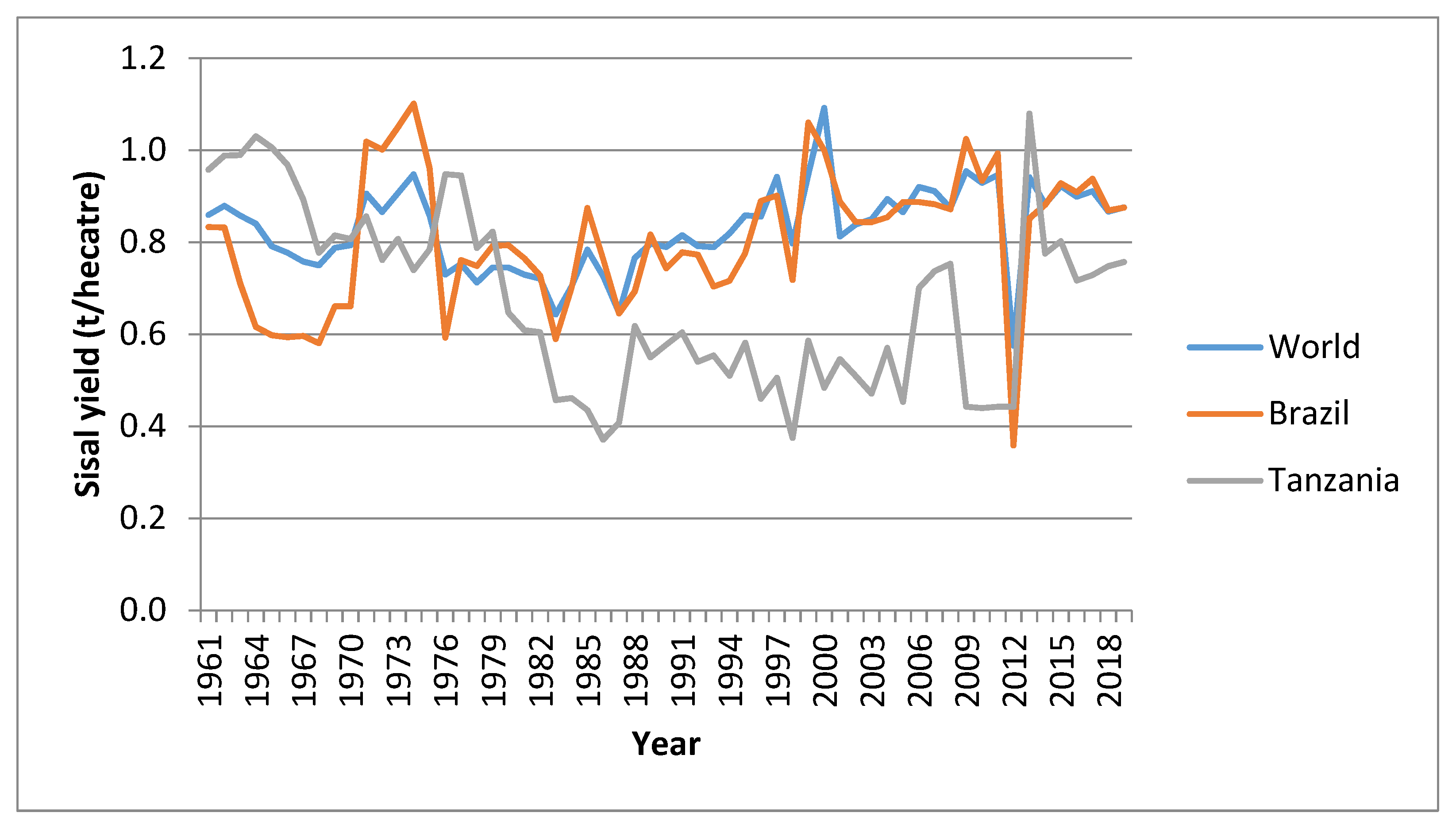
Appendix A.3. Historical Global Sisal Production Rates and Yield from FAO Data

During the 1960s, Tanzania was the world’s largest producer of sisal and export earnings from sisal contributed to 33% of the country’s foreign exchange income [62]. Tanzanian production peaked in 1964 with 233,540 tonnes produced from 226,620 hectares, which equates to approximately 26% of total world production [68] as indicated in Figure A1. Brazil has been the largest sisal producer since it overtook Tanzania in the 1970s, and now contributes to 56% of global production. During 2019, Tanzania was the second largest producer, with 29,563 tonnes produced from 38,108 hectares, which equates to 12% of global production, while Kenya produced 9% of global production.

Figure A1. Global Sisal Production from 1961 until 2019, showing a decrease in the 1970s [2].

Research efforts from the 1940s and 1950s produced a hybrid variety of sisal in the 1960s, known as Hybrid 11648, which produced nearly twice as much fiber per hectare as Agave sisalana [69] but was more susceptible to diseases and pests, particularly if there were deficiencies in nutrients such as calcium, phosphorus, and potassium [61]. Initially, annual fiber yields were > 1.5 tonnes per hectare for Agave sisalana and 2–3 tonnes per hectare for Hybrid 11648 [11,12], but gradually the yields decreased as indicated in Figure A2. FAO sisal yield records started in 1961, by which time sisal had been produced in certain areas of Tanzania for 60 years. During 2019, the average global yield was 0.88 tonnes per hectare, Tanzanian production averaged 0.76 tonnes per hectare, and Brazilian production averaged 0.88 tonnes per hectare as shown in Figure A2.

Figure A2. Sisal yields from start of record keeping in 1961 until 2019, showing Brazilian, Tanzanian, and average worldwide variation [2].

Appendix A.4. Sisal Composition

Data published on the estimated nutrient composition of sisal leaves varies [3,70,71] and has been based on nutrient removal from soil relative to fiber production, which does not indicate the mass composition of sisal leaves, given that the total fiber fraction can vary. Table 1 provides data on the nutrient content of sisal leaves based on the weight of seedlings produced in a nursery and indicates that calcium is found in the highest concentrations, but potassium, nitrogen, magnesium, and phosphorus are also important.

Table A1. Sisal fiber leaf nutrient composition calculated from nutrient removal from soil for seedlings in nursery and sisal in plantations.

Nutrient	Nursery Leaves ^a		Plantation Leaves ^b
Nutrient	Weight %	Ratio vs. N	Weight %	Ratio vs. N
Calcium	0.44	2.7	0.32	3.5
Magnesium	0.06	0.4	0.09	1.3
Nitrogen	0.16	1	0.12	1
Phosphorus	0.05	0.3	0.01	0.15
Potassium	0.18	1.1	0.14	1.5

Notes: ^a: estimate from nutrient decrease in nursery soil [14], ^b: estimate from nutrient decrease in soil from plantation after third cultivation cycle [11].

There are differences between the nutrient composition of Agave sisalana and Hybrid 11648, as indicated by the ratio relative to nitrogen, shown in Table A2. This indicates that Hybrid 11648 uses more calcium, significantly less potassium, and less phosphorus but that the nitrogen requirement is relatively similar.

Table A2. Nutrient removal and ratio relative to nitrogen (N) for Agave sisalana vs. Hybrid 11648, adapted from [14].

Nutrient	Agave Sisalana		Hybrid 11648
	kg Removed/ha.t Fiber	Relative to N	kg Removed/ha.t Fiber	Relative to N
Calcium	70	2.6	82	3.2
Magnesium	34	1.3	31	1.2
Nitrogen	27	1.00	26	1.0
Phosphorus	7	0.26	3.5	0.13
Potassium	69	2.6	44	1.7

Appendix B

Table A3. Life Cycle Inventory.

Process	Flow	BPS	IAS		Ecoinvent Process Used/Reference
1. Nursery and seedling preparation inventory
	Growing time (years)	1.5
	Bulbil planting density (#/ha)	100,000	80,000
	Weight of bulbil (kg)	0.06			Estimated from seedling size (9 cm vs. 35 cm)
	Bulbil loss rate	10%			[1]
	Glyphosate use (kg/ha)	2–3	0
	Glyphosate in roundup (g/L)	360	n/a		glyphosate \| market for glyphosate
	# Applications of roundup (#/growing cycle)	1	0		application of plant protection product, by field sprayer \| application of plant protection product, by field sprayer
	Fraction of glyphosate to soil	75%			[72]
	Fraction of glyphosate to air	25%			[72]
	Ploughing: wheel tractor—diesel L/ha	10	8–10		modified Ecoinvent process—tillage, harrowing, by rotary harrow\|tillage, harrowing, by rotary harrow\|APOS, U (TZ 1)
	Leveling: wheel tractor, harrow—diesel L/ha	10	8–10		modified Ecoinvent process—tillage, ploughing\|tillage, ploughing [APOS, U (TZ1)—RoW]
	Occupation, arable, non-irrigated				Reusing existing land, not clearing new land
	Agricultural lime use (kg/ha)	100	0		limestone, crushed, washed\|market for limestone, crushed, washed
	Calcium mass % in agricultural limestone	40%	n/a
	# Applications of agricultural lime (#/growing cycle)	1	0		done at same time as Muriate of potash
	Muriate of potash use (kg/ha)	5–9	0		potassium chloride, as K₂O\|market for potassium chloride, as K₂O
	# Applications of muriate of potash (#/growing cycle)	1	0		fertilizing, by broadcaster\|fertilizing, by broadcaster
	Potassium mass % in muriate of potash	50%
	Potassium mass % in K₂O	83%
	Distance—Dar es Salem port to nursery for inputs (km)	300	356
	Transport inputs—road—(glyphosate, lime, potash) (tkm)	32.85	0		transport, freight, lorry 16–32 metric ton, EURO3\|market for transport, freight, lorry 16–32 metric ton, EURO3
Output	Weight of seedling ready for planting (kg)	0.25
	Seedlings produced per hectare	90,000	72,000
2. Plantation
	Land preparation
	Brush cutting (L diesel used/hectare)—clearing	44	25		Modified Ecoinvent process—mowing, by rotary mower\|mowing, by rotary mower (TZ 2 clear)
	Burning of biomass material (25 t biomass/hectare, 10.4 GJ/t, green and air dried wood)—N₂O emissions 0.004 kg N₂O released/GJ biomass burnt, methane emission 0.028 kg methane released/GJ biomass burnt				Data from Table 2.2.2, p80, carbon dioxide not counted [73]
	Ploughing of burnt biomass material into soil, caterpillar with plough—diesel use (L) per hectare	36	0		Modified Ecoinvent process: tillage, ploughing\|tillage, ploughing\|APOS, U (TZ 2)—RoW
	Leveling: Caterpillar with harrowing	33	0		Modified Ecoinvent process: tillage, harrowing, by rotary harrow\|tillage, harrowing, by rotary harrow\|APOS, U (TZ 2)
	Leveling: Wheel tractor	0	18		Modified Ecoinvent process: tillage, harrowing, by rotary harrow\|tillage, harrowing, by rotary harrow\|APOS, U (TZ 2)
	Distance, nursery to plantation (km)	7	5		transport, tractor and trailer, agricultural \| market for transport, tractor and trailer, agricultural
	Distance, plantation to fiber processing (km)	10	7		transport, freight, lorry, all sizes, EURO3 to generic market for transport, freight, lorry, unspecified\|transport, freight, lorry, unspecified \| APOS, S—RoW
	Seedling planting density (#/ha)	5000	4000
	Growing cycle (years)	10–12	10–12
	Year of first harvest	3–4	3
	Years of harvesting per growing cycle	8–10	8–10
	Agricultural lime use (kg/ha)	5000	0		limestone, crushed, washed\|market for limestone, crushed, washed
	Calcium mass % in agricultural limestone	40%
	# Applications of agricultural lime (#/growing cycle)	1	0
	Triple Superphosphate (TSP) use (kg/ha)	100–125	0		phosphate fertilizer, as P₂O₅\|triple superphosphate production
	Phosphorus mass % in TSP	20%
	Calcium mass % in TSP	15.5%
	# Applications of TSP (#/growing cycle)	2	0		fertilizing, by broadcaster\|fertilizing, by broadcaster
	Composted sisal residue use (kg/ha)	300	0
	# Applications of composted sisal residues (#/growing cycle)	2	0
	Weeding—times, years 0–3	6	6		Modified Ecoinvent process—tillage, harrowing, by spring tine harrow\|tillage, harrowing, by spring tine harrow\|APOS, U (TZ 2)—RoW
	Weeding—times, years 4–6	4	6		Modified Ecoinvent process—mowing, by rotary mower \| mowing, by rotary mower (TZ 2 mow)
	Carbon dioxide uptake by plant material	Calculation based on 42% C in fiber [74]
	Mass of sisal ball at end of growing cycle (kg)	20	20		Included in biomass material burnt as part of field prep
	Distance—to Dar es Salaam from South Africa for TSP (km)	3100		n/a
	Distance—Port to plantation (km)	70		356	Note—different port to fiber export for BPS
	Occupation, arable, non-irrigated (ha.a)	1× growing cycle			Reusing existing land, not clearing new land
3. Fiber processing (both plants) & biogas plant (for BPS plant only)
	Yield, total fiber per hectare for year (t/year)	1.6	0.6		A—[4]
	Total fiber fraction in sisal leaves	4%	2.5%		B—assumed value
	Export fiber percent of total fiber	92%	59%		C—[4]
	Net export fiber yield (t/ha.year)	1.5	0.35		D = A x C
	Off-spec fiber yield (t/ha.year)—included as a negative input	0.1	0.25		A–D—entered as jute fiber\|market for jute fiber
	Sisal leaf production (t/ha.year)	40	24		E = A/B
	Sisal leaf production (t/ha.growing cycle)	340	204		F = E x years of harvesting
	Export fiber yield (t/ha.growing cycle)	12.5	3.0		G = D x years of harvesting
	Water usage, L/ton dry fiber	112,000	100,000
	Electricity use (kWh/t fiber) (refer to Appendix D for details on BPS)	615	343		BPS based on metered data, includes biogas plant, in theory should only be 30% higher than ordinary plant. IAS based on diesel genset (200L diesel to process 2.5 t fiber, assume 40% electrical efficiency)
	Note that estates will measure the tonnes of final product and estimate the weight of sisal leaves, so this is an area of potential data improvement
	Water content of total fiber entering drying process	60%
	Water content of total fiber leaving drying process	10–15%
	Ratio of sisal fiber residue to sisal export fiber	19	19
	Distance to port for sisal export grade fiber (km)	300	356
4. Sisal residue management
	Depth of ponds	1.5–3 m
	Engine electrical efficiency, biogas use	35%	-

Table A4. Supplementary information for life cycle inventory relating to electricity consumption at BPS. (Detailed information on electricity system based on installed capacity and running hours.)

	PLACE		#	kW	h/Day	kWh/Day (Calculated)	Subtotal	% of A or B	% of Total
A+B	BPS + biogas plant				Total	2896.0
A	BPS			Subtotal		2047.2			71%
A.1	CORONA	Corona motor	1	90	10	900
		Rope system motor	1	7.5	10	75
		Feed table motor	1	3.75	10	37.5
		Lamps	5	0.085	12	5.1
							1018	50%	35%
A.2	BRUSHING ROOM	Brushing machine motor	3	7.5	12	270
		Brushing machine motor	2	8	12	198
		Lamp	7	0.085	12	7.14
							475	23%	16%
A.3	BALING	Press pump motor	1	12	8	96
A.3	BALING	Lamp	4	0.085	8	2.72
							99	5%	3%
A.4	WORKSHOP	Motors	2	7.5	12	180
		Motor	1	5	12	60
		Lamp	2	0.085	2	0.34
							240	12%	8%
A.5	PUMP STATION	Pump motor	1	15.5	12	186
A.5	PUMP STATION	Lamp	3	0.085	12	3.1
							189	9%	7%
A.6	OFFICE	Lamp	18	0.085	2	3.1
A.7	SECURITY LAMP		4	0.085	12	4.1
A.8	Workers Houses	Room Lamps	120	0.02	4	9.6
A.8	Workers Houses	Security Lamp	40	0.02	12	9.6
B	BIOGAS PLANT				Subtotal	849			29%
B.1	CONVEYORS	Conveyor Motor	3	1.5	10	45
		Conveyor Motor	1	5.5	10	55
		Lamp	2	0.085	12	2.0
B.2	SQUEEZER	Squeezer motor	1	18.5	10	185
B.3	CAGE	Cage motor	1	7.5	10	75
B.4	COLLECTION TANK	Collection tank stirrer motor	1	5.5	10	55
B.4	COLLECTION TANK	Feed Pump	1	5	10	50
B.5	HYDROLYSIS	Stirrer motor	1	4	6	24
B.5	HYDROLYSIS	Feed Pump	1	15	6	90
B.6	DIGESTER	Stirrer motor	1	15	6	90
B.7	FERTILIZER TANK	Stirrer motor	1	15	6	90
B.8	H₂S CLEANER	Water pump	1	1.5	1	1.5
B.9	CHP	Water circulation pump	2	3	10	60
B.10	COOLING TOWER	Blower motor	1	1.5	10	15
B.11	MeS Office	Lamp	12	0.038	2	0.9
B.12	MeS Security lamp	Lamp	11	0.038	12	5.0
	Computers	Computers	2	0.02	6	0.2
	Refrigerator	Refrigerator	1	0.3	12	3.6
	Oven	Oven	1	0.3	5	1.5

Table A5. Assumption used to accentuate differences in yield in sisal production (not actual plant data), derived from [4].

Assumptions	Unit	BPS	IAS
Harvest years per growing cycle	years	8.5	8.5
Total fiber fraction of the leaves	%	4	2.5
Total fiber yield (export + off-spec)	t/ha/year	1.6	0.6
Export fiber yield	% total fiber yield	92	59
Calculated values
Total weight leaves grown	t/ha/year	40	24
Total weight leaves grown	t/ha/growing cycle	340	204
Total export fiber	t/ha/growing cycle	12.5	3.0
Total off-spec fiber	t/ha/growing cycle	1.1	2.1

Table A6. C:N ratio of total sisal waste stream.

	Unit	Sisal Pulp ^a	Sisal Wastewater ^b	Combined Sisal Waste
Mass per t sisal fiber	kg	15,490	121,472	136,962
% of total mass		11%	89%
Total solids (TS)	% of M	9%	1.6%	2.4%
Mass of TS	kg	1394	1944	3338
Volatile solids (VS)	% of TS	87.5%	47.7%	64%
Mass of VS	kg	1220	927	2147
Organic carbon (OC)	%	49%	39.3%	40%
Mass of OC	kg	683	364	1047
Total nitrogen (TN)	% of TS	1.08%	2.60%	1.97%
Mass of TN	kg	15.1	50.5	65.6
N partitioning ^c	%	23%	77%
Mass of TN	kg	From mass balance of sisal leaves		24.5
C:N ratio				59

Notes: ^a: [27]; ^b: [42]; same mass ratio between pulp & wastewater as in [4]; ^c: this indicates that more of the nitrogen seems to partition into the solid waste stream (23%) compared to the value used on a mass basis (11%).

Table A7. Life cycle assessment overview as per International Reference Life Cycle Data System (ILCD) Handbook for LCA [29].

Goal

Intended application is to assist with greening the sisal supply chain, steps required are:
(1)
develop a blueprint for applying circular economy principles to agribusiness supply chains, using LCA as a screening tool;
(2)
assess the extent of nutrient depletion in current sisal production by undertaking mass balances on five key nutrients using parameters within an LCA model;
(3)
calculate how much land can be made available if sisal yields are increased;
(4)
assist with identifying data required for a more comprehensive assessment.
Limitations due to the method, assumption, and impact coverage:
-
assumptions such as sisal composition under varying soil nutrient levels, link between nutrient levels and yields, composition of cosubstrates in Tanzanian economy, current use of cosubstrates (including whether current degradation is occurring anaerobically and whether nutrients are currently being discharged to environment), exact C:N required for anaerobic digestion of each cosubstrate with sisal residue, actual wet and dry deposition of key nutrients (particularly if this will change with climate change);
-
methodological issues such as behavior of nutrients (particularly nitrogen) in nutrient depleted soils within LCA modeling, given that LCA models were developed based on European and North American agricultural systems in which nutrients are most often in surplus);
Reasons for conducting the study:
(1)
assess potential for LCA to contribute to greening agribusiness supply chains, using LCA as a screening tool for various future development scenarios;
(2)
use LCA to assess nutrient depletion in agricultural system by using a mass balance within the LCA software;
(3)
as part of a larger PhD project on using LCA in SMEs in agribusiness supply chains;
(4)
address a key industry within the Tanzanian economy.
Decision content—Situation A, “micro-level decision support”—greening the supply chain (attributional) but with substitution rather than allocation.
Target audience of the deliverables/results:
(1)
for blueprint—policy makers, possibly other researchers in agribusiness fields, particularly those researching nutrient depletion and yield;
(2)
for LCIA results—researchers who will perform further work based on primary data (once it is available);
Comparative studies—not required, as not being used to make disclosure to public or consumers.
Commissioner of the study and other influential actors—PhD student at DTU and colleague from Sokoine University in Tanzania.

Scope

-: Type of deliverables—nutrient balances, LCI and LCIA results, presented in a journal article;
-: Functional unit—1 metric t sisal export fiber;
-: System boundaries—sisal nursery, plantation, fiber processing, waste management and transport to export port in Tanzania. Cosubstrate transport to site, anaerobic digestion of sisal waste and cosubstrate;
-: Coproducts handled by substitution e.g., sisal off-spec fiber substituted with jute, nutrients in cosubstrates substituted with equivalent amount of manufacturer fertilizer;
-: LCIA impact categories—17 midpoint impact categories—agricultural land occupation, climate change, fossil depletion, freshwater ecotoxicity, freshwater eutrophication, human toxicity, ionizing radiation, marine ecotoxicity, marine eutrophication, metal depletion, natural land transformation, ozone depletion, particulate matter formation, photochemical ozone formation, terrestrial acidification, terrestrial ecotoxicity, and water depletion;
-: Software—openLCA v 1.5.0, open LCA LCIA methods 1.5.2;
-: Database—Ecoinvent v3.2;
-: Primary data—site visits to Hale (BPS) and Mkumbara (IAS) provided most Life Cycle Inventory data on foreground system;
-: Secondary data—data on yield taken from recent article [4], highest yield relates to BPS, lower yield used for IAS to accentuate difference, data on sisal and cosubstrate composition taken from literature, other background data taken from Ecoinvent database.

Appendix C. Circular Economy in Tanzania—Identification of Potential Cosubstrates

The top ten agricultural products in Tanzania during 2019 in terms of tonnes produced (out of a national crop production total of 39,824,519 tonnes) are presented in Figure A3 and were cassava (21%), maize (14%), sweet potatoes (10%), sugar cane (9%), paddy rice (9%), bananas (9%), and vegetables (6%) [26].

Figure A3. Crop production in Tanzania in 2019, showing the total production, largest tonnage crops, and yield for each crop [26]. In terms of livestock production in Tanzania that may have organic residues that can be recycled to the sisal supply chain, the cow milk (77%) and beef meat (13%) sectors are by far the most significant, as indicated Figure A4.

Figure A4. Livestock Production in Tanzania in 2019 [26].

In addition to livestock production from farms, Figure A5 provides data on total meat production in Tanzania during 2018 and this indicates that freshwater and marine fish are significant meat sources.

Figure A5. Meat production in Tanzania in 2018 [26].

Appendix D. Life Cycle Impact Assessment Results (Note—Red Indicates Highest Value (Worst), Green Lowest (Best), Blue is the Second Lowest (Second Best)

Table A8. Detailed LCIA results for BPS, no current beneficial reuse of cosubstrate, raw data.

BPS			Cosubstrate with No Current Beneficial Reuse						Sink	Source
Impact Category (17)	Reference Unit	Current	DM	DM	CM	MFPW	HF	HU	Sink	Source
Agricultural land occupation	m²*a	−6.0	−45	−50	−46	−46	−45	−45	7	0
Climate change	kg CO₂-eq	29,945	−3198	−3533	−3277	−3309	−3229	−3246	6	1
Fossil depletion	kg oil eq	−1473	−1105	−1227	−1136	−1149	−1118	−1124	7	0
Freshwater ecotoxicity	kg 1,4-DB eq	−1.2	−6.8	−9.9	−8.4	−9.1	−7.5	−7.8	7	0
Freshwater eutrophication	kg P eq	3.2	3.7	3.8	3.6	3.6	3.6	3.6	0	7
Human toxicity	kg 1,4-DB eq	−31	−133	−255	−201	−229	−160	−175	7	0
Ionizing radiation	kg U235 eq	−14	−86	−114	−99	−105	−91	−94	7	0
Marine ecotoxicity	kg 1,4-DB eq	−0.92	−3.6	−7.6	−5.9	−6.8	−4.5	−5.0	7	0
Marine eutrophication	kg N eq	15	−43	−50	−42	−49	−45	−33	6	1
Metal depletion	kg Fe eq	−2.9	−11	−24	−19	−21	−14	−16	7	0
Natural land transformation	m²	−0.12	−0.85	−0.99	−0.90	−0.92	−0.87	−0.89	7	0
Ozone depletion	kg CFC-11 eq	−0.00004	−0.0003	−0.00036	−0.00033	−0.00034	−0.00031	−0.00032	7	0
Particulate matter formation	kg PM10 eq	2.0	2.7	3.3	2.9	3.6	3.5	2.2	0	7
Photochemical oxidant formation	kg NMVOC	11	−6.7	−9.5	−8.1	−8.7	−7.2	−7.6	6	1
Terrestrial acidification	kg SO₂ eq	18	34	44	39	45	42	32	0	7
Terrestrial ecotoxicity	kg 1,4-DB eq	−0.04	−0.08	−0.29	−0.21	−0.26	−0.13	−0.16	7	0
Water depletion	m³	−1763	−14,581	−14,708	−14,097	−13,900	−14,390	−14,284	7	0
Worst		14	0	1	0	2	0	0
Best		3	0	14	0	0	0	0
Sink		11	14	14	14	14	14	14	95
Source		6	3	3	3	3	3	3		24

Table A9. Detailed LCIA results for BPS, with current beneficial reuse of cosubstrate as fertilizer.

BPS			Cosubstrate with Current Beneficial Reuse						Sink	Source
Impact Category (17)	Reference Unit	Current	DM	BM	CM	MFPW	HF	HU	Sink	Source
Agricultural land occupation	m²*a	−6.0	−2.2	−3.1	−8.9	−16	1.3	−22	6	1
Climate Change	kg CO₂-eq	29,945	−2656	−2903	−2738	−2739	−2616	−2858	6	1
Fossil depletion	kg oil eq	−147	−1023	−1131	−1051	−1069	−1015	−1070	7	0
Freshwater ecotoxicity	kg 1,4-DB eq	−1.2	−0.03	−2.0	−1.3	−2.6	1.2	−3.3	6	1
Freshwater eutrophication	kg P eq	3.2	14	16	18	8.4	26	6.9	0	7
Human toxicity	kg 1,4-DB eq	−31	33	−60	−23	−73	59	−67	5	2
Ionizing radiation	kg U235 eq	−14	−61	−84	−72	−82	−57	−79	7	0
Marine ecotoxicity	kg 1,4-DB eq	−0.92	3.0	−0.02	0.98	−0.54	3.8	−0.67	4	3
Marine eutrophication	kg N eq	15	1.8	2.2	1.9	2.1	2.1	1.6	0	7
Metal depletion	kg Fe eq	−2.9	26	20	21	16	33	9.8	1	6
Natural land transformation	m²	−0.12	−0.77	−0.90	−0.82	−0.85	−0.77	−0.83	7	0
Ozone depletion	kg CFC-11 eq	−0.00004	−0.00027	−0.00032	−0.00029	−0.00030	−0.00027	−0.00029	7	0
Particulate matter formation	kg PM10 eq	2.0	3.6	4.4	3.9	4.4	4.8	2.8	0	7
Photochemical oxidant formation	kg NMVOC	11	−5.4	−7.9	−6.8	−7.4	−5.7	−6.7	6	1
Terrestrial acidification	kg SO₂ eq	18	37	48	42	48	45	34	0	7
Terrestrial ecotoxicity	kg 1,4-DB eq	−0.04	0.32	0.13	0.10	−0.05	0.27	0.02	2	5
Water depletion	m³	−1763	−13,903	−13,909	−13,342	−13,312	−13,426	−13,878	7	0
Worst		8	1	1	0	0	7	0
Best		5	0	7	0	2	0	3
Sink		11	9	11	10	12	7	11	71
Source		6	8	6	7	5	10	6		48

Table A10. Detailed LCIA results for IAS, with no current beneficial reuse of non-agricultural cosubstrates and current beneficial reuse of agricultural cosubstrates (manure).

IAS—Fusion			Cosubs with No Current Bene. Reuse			Cosubs with Current Bene. Reuse			Sink	Source
Impact Category	Reference Unit	Current	MFPW	HF	HU	DM	BM	CM	Sink	Source
Agricultural land occupation	m²*a	0	−63	−59	−60	49	48	33	3	3
Climate Change	kg CO₂ eq	41,049	−4458	−4256	−4300	−2807	−3426	−3005	6	1
Fossil depletion	kg oil eq	0	−1548	−1468	−1485	−1229	−1502	−1297	6	1
Freshwater ecotoxicity	kg 1,4-DB eq	0	−12	−7.9	−8.8	11	6.1	7.9	3	3
Freshwater eutrophication	kg P eq	8.2	3.4	4.1	3.6	29	35	41	0	7
Human toxicity	kg 1,4-DB eq	0	−297	−122	−160	365	133	226	3	3
Ionizing radiation	kg U235 eq	0	−139	−106	−113	−28	−86	−56	6	0
Marine ecotoxicity	kg 1,4-DB eq	0	−8.8	−2.8	−4.1	16	8.5	11	3	3
Marine eutrophication	kg N eq	39	−126	−114	−85	4.2	4.8	4.2	3	4
Metal depletion	kg Fe eq	0	−28	−9.1	−13	93	78	80	3	3
Natural land transformation	m²	0	−1.2	−1.1	−1.1	−0.86	−1.2	−0.98	6	0
Ozone depletion	kg CFC-11 eq	0	0.00	0.00	0.00	0.00	0.00	0.00	6	0
Particulate matter formation	kg PM10 eq	6.6	10	10	6.8	12	12	11	0	7
Photochemical oxidant formation	kg NMVOC	17	−11	−7.8	−8.6	−3.0	−9.6	−6.6	6	1
Terrestrial acidification	kg SO₂ eq	50	103	94	69	91	110	95	0	7
Terrestrial ecotoxicity	kg 1,4-DB eq	0	−0.33	0.00	−0.07	1.1	0.65	0.58	2	3
Water depletion	m³	0	−18,877	−20,118	−19,847	−18,883	−18,899	−17,458	6	0
Worst		8	0	0	0	6	2	1
Best		2	14	1	0	0	0	0
Sink		0	14	13	14	7	7	7	62
Source		6	3	4	3	10	10	10		46

Table A11. Process contribution for IAS, MFPW cosubstrate, no current beneficial use (2% cut-off).

Process Unit →		Electricity, High Voltage, Production Mix\|Electricity, High Voltage\|APOS, S–TZ	Treatment of Scrap Steel, Municipal Incineration\|Scrap Steel\|APOS, U–RoW	SRM–Fish Waste (RF = 1t Sisal Export Fiber]	Treatment of Brake Wear Emissions, Lorry\|Brake Wear Emissions, Lorry\|APOS, U–RoW
Impact Category ↓
Agricultural land occupation	m²*a	−47
	%	−101%
Climate change	kg CO₂ eq	−33,452
	%	−101%
Fossil depletion	kg oil eq	−1162
	%	−101%
Freshwater ecotoxicity	kg 1,4-DB eq	−9.4
	%	−103%
Freshwater eutrophication	kg P eq			3.7
	%			102%
Human toxicity	kg 1,4-DB eq	−2417			5.1
	%	−105%			2.2%
Ionizing radiation	kg U235 eq	−108
	%	−103%
Marine ecotoxicity	kg 1,4-DB eq	−7.4	0.1
	%	−106%	2.0%
Marine eutrophication	kg N eq			−49
	%			−99%
Metal depletion	kg Fe eq	−23
	%	−106%
Natural land transformation	m²	−0.94
	%	−102%
Ozone depletion	kg CFC-11 eq	−0.00035
	%	−102%
Particulate matter formation	kg PM10 eq	−4.5		8.0
	%	−127%		224%
Photochemical oxidant	kg NMVOC	−9.0
formation	%	−103%
Terrestrial acidification	kg SO₂ eq	−16.		61
	%	−37%		136%

References

Common Fund for Commodities and UNIDO. Sisal: Past Research Results and Present Production Practices, Amsterdam, 8. 2001. Available online: http://common-fund.org/fileadmin/user_upload/Publications/Technical/Hard_Fibres/CFC_Technical_Paper_No._8.pdf (accessed on 19 January 2017).
FAO. Sisal Production, 1961–2019. 2019. Available online: http://www.fao.org/faostat/en/#data/QC (accessed on 8 July 2021).
Lock, G.W. Sisal, 2nd ed.; Longmans: London, UK, 1969. [Google Scholar]
Broeren, M.L.M.; Dellaert, S.N.C.; Cok, B.; Patel, M.K.; Worrell, E.; Shen, L. Life cycle assessment of sisal fibre–Exploring how local practices can influence environmental performance. J. Clean. Prod. 2017, 149, 818–827. [Google Scholar] [CrossRef]
Nandra, S.S. The Role of Chemical Analysis in Determining the Fertilizer Requirements of Crops, Research Bulletin No. 56; Mlingano: Tanga, Tanzania, 1971. [Google Scholar]
Nandra, S.S. Soil fertility status of the sisal growing areas in Tanzania. African Soils 1977, XIX, 58–66. [Google Scholar]
Van Kekem, A.J.; Kimaro, D.N. Soils of Amboni Sisal Estate and Their Potential for Sisal Growing. Site Evaluations and Appraisal Studies S4; Mlingano: Tanga, Tanzania, 1986. [Google Scholar]
Kimaro, D.N.; Van Kekem, A.J. Soils of Kikwetu Sisal Estate and Their Potential for Sisal and Alternative Crops (Reconnaissance Soil Survey Report R4); Mlingano: Tanga, Tanzania, 1987. [Google Scholar]
Kips, P.A.; Mbongoni, J.D.J.; Ndondi, P.M. Soils of Kwafungo Estate and Their Suitability for Selected Fruit Crops and Hybriud Sisal Cultivation. Semi-Detailed Soil Survey Report D17; Mlingano: Tanga, Tanzania, 1989. [Google Scholar]
Ngailo, J.A.; Ndondi, P.M.; Kips, P.A. Soil Conditions and Agricultural Potential for Hybrid Sisal and Selected Fruit Crops at Kwamgwe Estate, Site Evaluations and Appraisal Studies S14; Mlingano: Tanga, Tanzania, 1990. [Google Scholar]
Hartemink, A.E.E.; Van Kekem, A.J. Nutrient depletion in Ferralsols under hybrid sisal cultivation in Tanzania. Soil Use Manag. 1994, 10, 103–107. [Google Scholar] [CrossRef]
Hartemink, A.E.; Wienk, J.F. Sisal Production and Soil Fertility Decline in Tanzania. Outlook Agric. 1995, 24, 91–96. Available online: http://www.alfredhartemink.nl/PDF/1995-SisalproductionTanzania.pdf (accessed on 19 January 2017). [CrossRef]
Hartemink, A.E.; Osborne, J.F.; Kips, P.A. Soil Fertility Decline and Fallow Effects in Ferralsols and Acrisols of Sisal Plantations in Tanzania. Expl. Agric. 1996, 32, 173–184. Available online: http://www.alfredhartemink.nl/PDF/1996-Falloweffectsandsoilfertilitydecline.pdf (accessed on 19 January 2017). [CrossRef]
Hartemink, A.E. Input and output of major nutrients under monocropping sisal in Tanzania. Land Degrad. Dev. 1997, 8, 305–310. [Google Scholar] [CrossRef]
Hartemink, A.E. Soil fertility decline in some Major Soil Groupings under permanent cropping in Tanga Region, Tanzania. Geoderma 1997, 75, 215–229. Available online: http://www.alfredhartemink.nl/PDF/1997-SisalTanzania.pdf (accessed on 19 January 2017). [CrossRef]
FAO. The Future of Food and Agriculture—Alternative Pathways to 2050, Rome. 2018. Available online: http://www.fao.org/3/I8429EN/i8429en.pdf (accessed on 14 January 2019).
United Nations. World Population Prospects: The 2015 Revision, Key Findings and Advance Tables; United Nations: New York, NY, USA, 2015. [Google Scholar] [CrossRef]
International Energy Agency (IEA). World Energy Outlook 2019, 2019th ed.; International Energy Agency: Washington, DC, USA, 2019; ISBN 978-92-64-97300-8. [Google Scholar]
International Energy Agency (IEA), IEA Country Profile—Tanzania, Country Profiles. 2019. Available online: https://www.iea.org/countries/tanzania (accessed on 8 July 2021).
Terrapon-Pfaff, J.C.; Fischedick, M.; Monheim, H. Energy potentials and sustainability—The case of sisal residues in Tanzania. Energy Sustain. Dev. 2012, 16, 312–319. [Google Scholar] [CrossRef] [Green Version]
Kivaisi, A.; Rubindamayugi, M.S.T. The potential of agro-indsutrial residues for production of biogas and electricity in Tanzania. Renew. Energy 1996, 9, 917–921. [Google Scholar] [CrossRef]
Jungersen, G.; Kivaisi, A.; Rubindamayugi, M. Bioenergy from Sisal Residues-Experimental Results and Capacity Building Activities (EFP-95 Project); 1998. Available online: https://www.etde.org/etdeweb/servlets/purl/632768/?type=download (accessed on 19 January 2017).
Geissdoerfer, M.; Morioka, S.N.; de Carvalho, M.M.; Evans, S. Business models and supply chains for the circular economy. J. Clean. Prod. 2018, 190, 712–721. [Google Scholar] [CrossRef]
Bocken, N.M.P.; de Pauw, I.; Bakker, C.; van der Grinten, B. Product design and business model strategies for a circular economy. J. Ind. Prod. Eng. 2016, 33, 308–320. [Google Scholar] [CrossRef] [Green Version]
Ellen MacArthur Foundation, Circular Economy Overview. 2015. Available online: https://www.ellenmacarthurfoundation.org/circular-economy (accessed on 17 January 2017).
FAO. FAOSTAT, Crops and Livestock Products. 2019. Available online: http://www.fao.org/faostat/en/#data/TP (accessed on 25 January 2019).
Mshandete, A.; Kivaisi, A.; Rubindamayugi, M.; Mattiasson, B. Anaerobic batch co-digestion of sisal pulp and fish wastes. Bioresour. Technol. 2004, 95, 19–24. [Google Scholar] [CrossRef] [PubMed]
Hills, D.J.; Roberts, D.W. Anaerobic digestion of dairy manure and field crop residues. Agric. Wastes 1981, 3, 179–189. Available online: http://production.datastore.cvt.dk/filestore?oid=532e0a01f36b9a657d0a263f&targetid=5326f8cdea081d6c09086cf7 (accessed on 12 January 2017). [CrossRef]
EC-JRC. (ILCD) Handbook: General Guide for Life Cycle Assessment—Detailed Guidance; Publications Office of the European Union: Luxembourg, 2010. [Google Scholar] [CrossRef]
Hauschild, M.Z.; Rosenbaum, R.K.; Olsen, S.I.; Bjørn, A.; Owsianiak, M.; Molin, C.; Laurent, A.; Ryberg, M.W.; Moltesen, A.; Corona, A.; et al. Life Cycle Assessment: Theory and Practice, 1st ed.; Hauschild, M.Z., Rosenbaum, R.K., Olsen, S.I., Eds.; Springer: Cham, Switzerland, 2017; ISBN 9783319564753. [Google Scholar]
Rockström, J.; Steffen, W.; Noone, K.; Persson, Å.; Chapin, F.S.; Lambin, E.; Lenton, T.M.; Scheffer, M.; Folke, C.; Schellnhuber, H.J.; et al. Planetary boundaries: Exploring the safe operating space for humanity. Ecol. Soc. 2009, 461, 4. [Google Scholar] [CrossRef]
Steffen, W.; Richardson, K.; Rockström, J.; Cornell, S.E.; Fetzer, I.; Bennett, E.M.; Biggs, R.; Carpenter, S.R.; De Vries, W.; De Wit, C.A.; et al. Planetary boundaries: Guiding human development on a changing planet. Science 2015, 347. [Google Scholar] [CrossRef] [Green Version]
Nemecek, T.; Kagi, T. Life Cycle Inventories of Agricultural Production Systems, Ecoinvent Report No. 15. Final Rep. Ecoinvent V2.0 2007, 1–360. Available online: http://www.upe.poli.br/~cardim/PEC/EcoinventLCA/ecoinventReports/15_Agriculture.pdf (accessed on 17 January 2017).
Muthangya, M.; Hashim, S.O.; Amana, J.M.; Mshandete, A.M.; Kivaisi, A.K.; Mutemi, M. Auditing and Characterisation of Sisal Processing Waste: A Bioresource for Value Addition. ARPN J. Agric. Biol. Sci. 2013, 8, 518–524. Available online: www.arpnjournals.com (accessed on 11 January 2017).
UNIDO and Common Fund for Commodities. Feasibility Study for the Generation of Biogas and Electricity from Sisal Waste—Construction and Ooperations Manual (Project No. US/URT/09/006-1151 and FB/URT/09/A04-1151); Common Fund for Commodities: Amsterdam, The Netherlands, 2010. [Google Scholar]
Stoorvogel, J.J.; Smaling, E.M.A. Volume III: Literature review and description of land use. In Assessment of Soil Nutrient Depletion in Sub Saharan Africa: 1983–2000; The Winand Staring Centre for Integrated Land, Soil and Water Research: Wageningen, The Netherlands, 1990. [Google Scholar]
Parker, G.G. Throughfall and stemflow in the forest nutrient cycle. Adv. Ecol. Res. 1983, 13, 57–133. [Google Scholar]
Nitrogen Deposition, Critical Loads and Biodiversity; Sutton, M.A.; Mason, K.E.; Sheppard, L.J.; Sverdrup, H.; Haueber, R.; Hicks, W.K. (Eds.) Springer: Berlin/Heidelberg, Germany; New York, NY, USA; London, UK, 2014; ISBN 9789400779389. [Google Scholar]
Cosme, N.; Hauschild, M.Z. Characterization of waterborne nitrogen emissions for marine eutrophication modelling in life cycle impact assessment at the damage level and global scale. Int. J. Life Cycle Assess 2017. [Google Scholar] [CrossRef] [Green Version]
Nerini, F.F.; Andreoni, A.; Bauner, D.; Howells, M. Powering production. The case of the sisal fibre production in the Tanga region, Tanzania. Energy Policy 2016, 98, 544–556. [Google Scholar] [CrossRef]
Salum, A.; Hodes, G. Leveraging CDM to Scale-Up Sustainable Biogas Production from Sisal Waste. Available online: https://backend.orbit.dtu.dk/ws/portalfiles/portal/4044107/Salum_paper.pdf (accessed on 13 March 2017).
Mshandete, A.; Björnsson, L.; Kivaisi, A.K.; Rubindamayugi, M.S.T.; Mattiasson, B. Effect of particle size on biogas yield from sisal fibre waste. Renew. Energy 2006, 31, 2385–2392. [Google Scholar] [CrossRef]
Mshandete, A.; Bjornsson, L.; Kivaisi, A.; Rubindamayugi, M.; Mattiasson, B. Performance of a sisal fibre fixed-bed anaerobic digester for biogas production from sisal pulp waste. Tanzania J. Sci. 2005, 31, 41–52. [Google Scholar] [CrossRef] [Green Version]
Muthangya, M.; Mshandete, A.M.; Kivaisi, A.K. Enhancement of Anaerobic Digestion of Sisal Leaf Decortication Residues By Biological Pre-Treatment. ARPN J. Agric. Biol. Sci. 2009, 4, 66–73. [Google Scholar]
Mshandete, A.; Björnsson, L.; Kivaisi, A.K.; Rubindamayugi, S.T.; Mattiasson, B. Enhancement of anaerobic batch digestion of sisal pulp waste by mesophilic aerobic pre-treatment. Water Res. 2005, 39, 1569–1575. [Google Scholar] [CrossRef] [PubMed]
Mshandete, A.M.; Björnsson, L.; Kivaisi, A.K.; Steven, M.; Rubindamayugi, T.; Mattiasson, B. Effect of aerobic pre-treatment on production of hydrolases and volatile fatty acids during anaerobic digestion of solid sisal leaf decortications residues. African J. Biochem. Res. 2008, 2, 111–119. Available online: http://www.academicjournals.org/AJBR (accessed on 13 March 2017).
Gumisiriza, R.; Mshandete, A.M.; Thomas, M.S.; Kansiime, F.; Kivaisi, A.K. Nile perch fish processing waste along Lake Victoria in East Africa: Auditing and characterization. African J. Environ. Sci. Technol. 2009, 3, 13–20. [Google Scholar] [CrossRef]
Foo, K. Value-added utilization of maize cobs waste as an environmental friendly solution for the innovative treatment of carbofuran. Process Saf. Environ. Prot. 2016, 1, 295–304. [Google Scholar] [CrossRef]
Ali Abro, S.; Tian, X.; Wang, X.; Wu, F.; Esther Kuyide, J. Decomposition characteristics of maize (Zea mays. L.) straw with different carbon to nitrogen (C/N) ratios under various moisture regimes. African J. Biotechnol. 2011, 10, 10149–10156. [Google Scholar] [CrossRef]
Kamolmanit, N.; Reungsang, A. Effect of carbon to ntirogen ratio on the composting of cassava pulp with swine manure. J. Water Environ. Technol. 2006, 4, 18. Available online: https://www.jstage.jst.go.jp/article/jwet/4/1/4_1_33/_pdf (accessed on 17 January 2017).
Suthar, S.; Mutiyar, P.K.; Singh, S. Vermicomposting of milk processing industry sludge spiked with plant wastes. Bioresour. Technol. 2012, 116, 214–219. [Google Scholar] [CrossRef] [PubMed]
Rusinamhodzi, L.; Murwira, H.K.; Nyamangara, J. Effect of cotton-cowpea intercropping on C and N mineralisation patterns of residue mixtures and soil. Aust. J. Soil Res. 2009, 47, 190–197. [Google Scholar] [CrossRef]
Esteban, M.B.; García, A.J.; Ramos, P.; Márquez, M.C. Evaluation of fruit–vegetable and fish wastes as alternative feedstuffs in pig diets. Waste Manag. 2006, 27, 193–200. [Google Scholar] [CrossRef] [PubMed]
Muñoz, I.; i Canals, L.M.; Clift, R.; Doka, G. A simple model to include human excretion and wastewater treatment in life cycle assessment of food products. Cent. Environ. Strateg. Univ. Surrey 2007, 1–46. Available online: http://www.doka.ch/CEShumanExcretion07.pdf (accessed on 13 March 2017).
Rose, C.; Parker, A.; Jefferson, B.; Cartmell, E. The Characterization of Feces and Urine: A Review of the Literature to Inform Advanced Treatment Technology. Crit. Rev. Environ. Sci. Technol. 2015, 45, 1827–1879. [Google Scholar] [CrossRef] [PubMed] [Green Version]
Strauss, M. Health Aspects of Nightsoil and Sludge Use in Agriculture and Aqua- Culture. Part II: Pathogen Survival (04/85); International Reference Centre for Waste Disposal (IRCWD): Duebendorf, Switzerland, 1985. [Google Scholar]
Felix, M. Status update on LCA studies and networking in Tanzania. Int. J. Life Cycle Assess. 2016, 21, 1825–1830. [Google Scholar] [CrossRef]
Lock, G.W. Sisal: Twenty-Five Years’ Sisal Research; Tropical, S., Ed.; Longmans, Green: London, UK, 1962. [Google Scholar]
Common Fund for Commodities. Discover Natural Fibres. 2009. Available online: http://www.fao.org/3/i0709e/i0709e00.htm (accessed on 19 January 2017).
Cantalino, A.; Torres, E.A.; Silva, M.S. Sustainability of Sisal Cultivation in Brazil Using Co-Products and Wastes. J. Agric. Sci. 2015, 7, 64–74. Available online: http://citeseerx.ist.psu.edu/viewdoc/summary?doi=10.1.1.958.7749 (accessed on 11 January 2017). [CrossRef] [Green Version]
Kimaro, D.N.; Msanya, B.M. Review of sisal production and research in Tanzania. Afr. Study Monogr. 1994, 15, 227–242. [Google Scholar]
Tambyrajah, D.; Patel, D.M.; Faaij, P.A. A Blueprint for a Sustainability Certification Scheme for The Hard Fibers Sector; Common Fund for Commodities: Amsterdam, The Netherlands, 2012; Available online: http://common-fund.org/fileadmin/user_upload/Projects/FIGHF/FIGHF_32FT/Final_Report_August_2012.pdf (accessed on 23 February 2017).
FAO and Common Fund for Commodities. Alternative Applications for Sisal and Henequen. In Technical Paper 14; 2001; p. 121. Available online: http://common-fund.org/fileadmin/user_upload/Publications/Technical/Hard_Fibres/Technical_Paper_No._14.pdf (accessed on 18 January 2017).
Common Fund for Commodities, “Product and Market Development of Sisal and Henequen,” Amsterdam. 2005. Available online: http://common-fund.org/fileadmin/user_upload/Publications/Technical/Hard_Fibres/CFC_FIGHF_07.pdf (accessed on 23 February 2017).
Magoggo, J.P. Cleaner Integral Utilization of Sisal Waste for Biogas and Biofertilizers; Common Fund for Commodities: Tanga, Tanzania, 2011; Available online: http://www.jpfirstlab.com (accessed on 3 February 2017).
Andrade, W. Feasibility Evaluation for Utilization of Sisal Liquid Waste (Juice) for the Production of Pesticides and Veterinary Drugs. Sindifibras, Brazil. 2012. Available online: http://common-fund.org/fileadmin/user_upload/Projects/FIGHF/FIGHF_30FT/Final_Report_2012.pdf (accessed on 19 January 2017).
Fortucci, P.; Mbabaali, S. Impact Evaluation of a CFC Funded Cluster of Sisal Projects; Common Fund for Commodities: Amsterdam, The Netherlands, 2015. [Google Scholar]
FAOSTAT. 2014 Sisal Production; FAO: Rome, Italy, 2014. [Google Scholar]
Hopkinson, D.; Wienk, J.F. Agave Hybrid Evaluations. In Tanganyika Sisal Growers’ Association Annual Report 1965/1966; Tanganyika Sisal Growers’ Association: Tanga, Tanzania, 1966. [Google Scholar]
Muller, A. Health status of sisal plants (Agave sisalana) as related to soils and the mineral composition of their leaves. J. Sci. Food Agric. 1964, 15, 129–132. [Google Scholar] [CrossRef]
Osborne, J.F. Some Preliminary Estimates of Nutrient Removal by Agave Crops; Tanganyika Sisal Growers’ Association: Mlingano, Tanzania, 1967. [Google Scholar]
Neto, B.; Dias, A.C.; Machado, M. Life cycle assessment of the supply chain of a Portuguese wine: From viticulture to distribution. Int. J. Life Cycle Assess. 2013, 18, 590–602. [Google Scholar] [CrossRef]
Department of the Environment and Energy. National Greenhouse Accounts Factors, Australian National Greenhouse Accounts; ACT: Canberra, Australia, 2016. Available online: www.environment.gov.au (accessed on 3 March 2017).
Salazar, V.L.P.; Leao, A.L. Biodegradation of coconut and sisal fibers applied in the automotive industry (in Portugese). Energy Agric. Botucatu 2006, 21, 99–133. [Google Scholar]

Figure 1. System boundary for LCA study of sisal supply chain in Tanzania.

Figure 2. IAS sink MICs—relative scoring of biodigester and generator scenarios compared to base case with no current beneficial reuse of cosubstrate (1 represents the best case, 0 the worst).

Figure 3. IAS source and sources-to-sink MICs—relative scoring of biodigester/generator scenarios compared to base case with no current beneficial reuse of cosubstrate (1 represents the best case, 0 the worst).

Figure 4. IAS sink MICs—relative scoring of biodigester/generator scenarios compared to base case with current beneficial reuse of cosubstrate (1 represents the best case, 0 the worst).

Figure 5. IAS non-sink MICs—relative scoring of biodigester/generator scenarios compared to base case with current beneficial reuse of cosubstrate (1 represents the best case, 0 the worst).

Figure 6. IAS sink MICs—Relative scoring of biodigester/generator scenarios compared to base case with current beneficial reuse of agricultural cosubstrates and no current beneficial reuse of non-agricultural cosubstrates (1 represents the best case, 0 the worst).

Figure 7. IAS non-sink MICs—Relative scoring of biodigester/generator scenarios compared to base case with current beneficial reuse of agricultural cosubstrates and with no current beneficial reuse of non-agricultural cosubstrates (1 represents the best case, 0 the worst).

Table 1. C:N ratios for wastes available in Tanzania (shading indicates that waste has a suitable C:N ratio).

	TN ^h %	TKN ^h %	TOC ^h %	Non-Lignin TOC%	TOC:TN	TOC:TKN	nlTOC:TKN
Maize cobs ^a	1.99		48.77		25
Maize straw ^b	0.86		42		49
Cassava pulp ^c	0.45		51.5		118
Rice hulls ^d		0.69	32.9	22.5		48	33
Rice straw ^d		0.39	33.6	28.9		86	74
Sugar cane trash ^e	2.52		49.15		15.5
Cowpea residue ^f	2.7		43.1		16.0
Grass clippings ^d		3.25	40.8	38.4		12.6	11.8
Dairy manure (DM) ^d		2.14	Table	29.6		19.1	13.8
Beef manure (BM) ^d		2.1	38.5	30		18	14
Chicken manure (CM) ^d		6.87	31.7	30.3		4.6	4.4
Pig manure ^d		3.67	44.3	39.7		12.1	10.8
Pig manure ^c	2.47		26.16		10.6
Milk proc sludge ^e	5.68		37.9		5.06
Marine fish waste (MFPW) ^g	5.85		51		9

Notes. ^a: [48]; ^b: [49]; ^c: [50]; ^d: [28]; ^e: [51]; ^f: cowpea residues from [52]; ^g: [27]; ^h: TN: total nitrogen, TKN: total Kjeldahl nitrogen; TOC: total organic carbon; nlTOC: non-lignin TOC.

Table 2. Estimate of mass and equivalent units of organic waste required to achieve C:N ratio of 25 for codigestion with total sisal waste stream at IAS for 1 t sisal export fiber.

	Unit	DM ^a	BM ^a	CM ^a	MFPW ^b	HF ^c	HU ^c,d
Mass required	kg	22,500	19,700	8150	2220	16,850	13,650
Equivalent animals or people/day		407	886	69,150	6343 ^e	69,342	9613
Nutrient input from cosubstrates
Calcium	kg	44	43	167	34	77	2
Magnesium	kg	19	17	18	1.0	15	1.9
Nitrogen	kg	113	132	110	130	118	87
Phosphorus	kg	25	31	37	12	56	8
Potassium	kg	77	73	41	4	64	17

Notes: ^a: [28]; ^b: fish waste assumed to be 35% of total fish mass [47,53]; ^c: TOC was assumed to be 47.9% of COD [54]; C and N are average of values reported in [55]; ^d: [56]; ^e: fish waste; the “equivalent animals” refers to the mass of marine fish required to produce the mass of waste, given that 35% of live fish ends up as waste.

Table 3. Estimate of mass and equivalent units of organic waste required to achieve C:N of 25 for codigestion with total sisal waste stream at BPS for 1 t sisal export fiber.

	Unit	DM	BM	CM	MFPW	HF	HU
C:N ratio		6.2	8.9	5.8	8.7	7.1	0.8
Mass required	kg	8900	7750	3200	875	6650	5400
Equivalent animals or people/day		161	349	27,134	2500	27,366	3808
Nutrient input from cosubstrates
Calcium	kg	17	17	65	13	30	0.7
Magnesium	kg	8	7	7	0.4	6	0.8
Nitrogen	kg	45	52	43	51	47	35
Phosphorus	kg	10	12	15	5	22	3
Potassium	kg	30	29	16	2	25	7

Table 4. Nutrient balances per tonne of export sisal fiber from nursery and plantation, BPS and IAS (negative values indicate depletion).

		Best Practice Site (BPS)			Industry Average Site (IAS)
Nutrient	Unit	Nursery	Plantation	Total	Nursery	Plantation	Total
Calcium	kg	−0.74	56	55	−7.1	−276	−283
Magnesium	kg	−0.18	−29	−30	−0.38	−68	−68
Nitrogen	kg	−0.52	−19	−19	−1.3	−36	−37
Phosphorus	kg	−0.26	−1.6	−1.9	−0.83	−7.3	−8.1
Potassium	kg	−0.80	−35	−36	−3.0	−84	−87

Table 5. Nutrients available from recycled waste compared to initial depletion for the IAS per tonne of sisal export fiber (bold text indicates that recycled waste provides nutrients in excess of initial depletion).

	Unit	DM	BM	CM	MFPW	HF	HU	Initial Depletion
Calcium	kg	128	128	252	118	161	86	−283
Magnesium	kg	50	48	49	32	46	33	−68
Total Nitrogen (TN)	kg	137	157	135	154	142	112	−37
Phosphorus	kg	29	35	41	15	60	12	−8
Potassium	kg	113	109	77	40	100	53	−87

Table 6. Nutrient available from recycled waste compared to initial depletion for the BPS per tonne of sisal export fiber (bold text indicates that recycled waste provides nutrients in excess of initial depletion).

	Unit	DM	BM	CM	MFPW	HF	HU	Initial Depletion
Calcium	kg	102	102	150	98	115	85	55
Magnesium	kg	39	38	38	32	37	32	−30
Nitrogen	kg	69	79	68	76	71	59	−19
Phosphorus	kg	14	16	18	8.3	26	6.9	−1.9
Potassium	kg	67	65	52	38	62	43	−36

Table 7. Detailed LCA results for the IAS biodigester and generator scenarios, with and without beneficial reuse of cosubstrates, per tonne of export fiber.

IAS	Reference Unit	Current Base Case	Cosubstrate with no Current Beneficial Reuse						Current Base Case	Cosubstrate with Current Beneficial Reuse
Impact Category (17)	Reference Unit	Current Base Case	DM	BM	CM	MFPW	HF	HU	Current Base Case	DM	BM	CM	MFPW	HF	HU
Agricultural land occupation	*m²a**	0	−58	−71	−61	−63	−59	−60	0	49	48	33	14	59	−1.7
Climate Change	kg CO₂ eq	41049	−4178	−5027	−4376	−4458	−4256	−4300	41049	−2807	−3426	−3005	−3013	−2703	−3318
Fossil depletion	kg oil eq	0	−1437	−1746	−1515	−1548	−1468	−1485	0	−1229	−1502	−1297	−1344	−1207	−1347
Freshwater ecotoxicity	kg 1,4-DB eq	0	−6.3	−14	−10	−12	−7.9	−8.8	0	11	6.1	7.9	4.6	14	2.5
Freshwater eutrophication	kg P eq	8.2	3.7	4.0	4.0	3.4	4.1	3.6	8.2	29	35	41	16	61	12
Human toxicity	kg 1,4-DB eq	0	−54	−362	−226	−297	−122	−160	0	365	133	226	100	431	111
Ionizing radiation	kg U235 eq	0	−93	−162	−126	−139	−106	−113	0	−28	−86	−56	−82	−19	−74
Marine ecotoxicity	kg 1,4-DB eq	0	−0.53	−11	−6.4	−8.8	−2.8	−4.1	0	16	8.5	11	7.2	18	6.7
Marine eutrophication	kg N eq	39	−109	−128	−107	−126	−114	−84	39	4.2	4.8	4.2	4.7	4.6	3.3
Metal depletion	kg Fe eq	0	−1.8	−34	−20	−28	−9.0	−13	0	93	78	80	67	110	51
Natural land transformation	m²	0	−1.1	−1.4	−1.2	−1.2	−1.1	−1.1	0	−0.86	−1.2	−0.98	−1.0	−0.86	−1.0
Ozone depletion	kg CFC-11 eq	0.0	−0.00035	−0.00052	−0.00042	−0.00045	−0.00038	−0.00040	0.0	−0.00027	−0.00042	−0.00033	−0.00037	−0.00028	−0.00034
Particulate matter formation	kg PM10 eq	6.6	9.3	9.7	8.8	10	10	6.8	6.6	12	12	11	13	13	8.3
Photochemical oxidant formation	kg NMVOC	17	−6.4	−13	−10	−11	−7.8	−8.6	17	−3.03	−9.6	−6.6	−8.2	−3.8	−6.4
Terrestrial acidification	kg SO₂ eq	50	84	101	87	102	94	69	50	91	110	95	110	103	74
Terrestrial ecotoxicity	kg 1,4-DB eq	0	0.13	−0.42	−0.19	−0.33	0.00	−0.07	0	1.1	0.65	0.58	0.19	1.0	0.38
Water depletion	m³	0	−20598	−20930	−19380	−18877	−20118	−19847	0	−18883	−18899	−17458	−17385	−17676	−18821

Publisher’s Note: MDPI stays neutral with regard to jurisdictional claims in published maps and institutional affiliations.

© 2021 by the authors. Licensee MDPI, Basel, Switzerland. This article is an open access article distributed under the terms and conditions of the Creative Commons Attribution (CC BY) license (https://creativecommons.org/licenses/by/4.0/).

Share and Cite

MDPI and ACS Style

Colley, T.A.; Valerian, J.; Hauschild, M.Z.; Olsen, S.I.; Birkved, M. Addressing Nutrient Depletion in Tanzanian Sisal Fiber Production Using Life Cycle Assessment and Circular Economy Principles, with Bioenergy Co-Production. Sustainability 2021, 13, 8881. https://0-doi-org.brum.beds.ac.uk/10.3390/su13168881

AMA Style

Colley TA, Valerian J, Hauschild MZ, Olsen SI, Birkved M. Addressing Nutrient Depletion in Tanzanian Sisal Fiber Production Using Life Cycle Assessment and Circular Economy Principles, with Bioenergy Co-Production. Sustainability. 2021; 13(16):8881. https://0-doi-org.brum.beds.ac.uk/10.3390/su13168881

Chicago/Turabian Style

Colley, Tracey Anne, Judith Valerian, Michael Zwicky Hauschild, Stig Irving Olsen, and Morten Birkved. 2021. "Addressing Nutrient Depletion in Tanzanian Sisal Fiber Production Using Life Cycle Assessment and Circular Economy Principles, with Bioenergy Co-Production" Sustainability 13, no. 16: 8881. https://0-doi-org.brum.beds.ac.uk/10.3390/su13168881

Note that from the first issue of 2016, this journal uses article numbers instead of page numbers. See further details here.

Article Menu

Addressing Nutrient Depletion in Tanzanian Sisal Fiber Production Using Life Cycle Assessment and Circular Economy Principles, with Bioenergy Co-Production

Abstract

1. Introduction

2. Materials and Methods

2.1. Circular Economy in Tanzania—Identifying Potential Cosubstrates and Nutrient Balances

2.2. LCA of Sisal Production, including Mass Balances to Assess Nutrient Depletion

3. Results and Discussion

3.1. Circular Economy in Tanzania—Potential Cosubstrates and Nutrient Balances

3.1.1. Potential Nutrient Sources from within the Tanzanian Economy

3.1.2. Nutrient Balances of Cosubstrates

3.2. LCA Results

3.2.1. Nutrient Balances of Current Operation

3.2.2. Nutrient Balances of Current Operation with Cosubstrates Added

3.2.3. LCA Results of Current Base Case

3.2.4. Results for the IAS Biodigester/Generator Scenarios

3.2.5. Results for the IAS with Current Beneficial Reuse of Agricultural Cosubstrate and No Current Beneficial Reuse for Non-agricultural Waste Cosubstrate

3.2.6. Significant Processes Contributing to MIC for the IAS

4. Conclusions

Author Contributions

Funding

Data Availability Statement

Conflicts of Interest

Appendix A. Background Information on Sisal

Appendix A.1. Sisal Production Methods in Tanzania

Appendix A.2. Historical Sisal Fiber Use

Appendix A.3. Historical Global Sisal Production Rates and Yield from FAO Data

Appendix A.4. Sisal Composition

Appendix B

Appendix C. Circular Economy in Tanzania—Identification of Potential Cosubstrates

Appendix D. Life Cycle Impact Assessment Results (Note—Red Indicates Highest Value (Worst), Green Lowest (Best), Blue is the Second Lowest (Second Best)

References

Share and Cite

Article Metrics

Article Access Statistics

Further Information

Guidelines

MDPI Initiatives

Follow MDPI