
Lane-Level Map-Aiding Approach Based on Non-Lane-Level Digital Map Data in Road Transport Security


Institute of Engineering Geodesy (IIGS), University of Stuttgart, D-70174 Stuttgart, Germany
*
Author to whom correspondence should be addressed.
Sustainability 2021, 13(17), 9724; https://0-doi-org.brum.beds.ac.uk/10.3390/su13179724
Submission received: 8 July 2021
/
Revised: 31 July 2021
/
Accepted: 11 August 2021
/
Published: 30 August 2021
(This article belongs to the Collection Emerging Technologies and Sustainable Road Safety)
Abstract
:To prevent terror attacks in which trucks are used as weapons as happened in Nice or Berlin in 2016, the European Project Autonomous Emergency Maneuvering and Movement Monitoring for Road Transport Security (TransSec) was launched in 2018. One crucial point of this project is the development of a map-aiding approach for the localization of vehicles on digital maps, so that the information in digital map data can be used to detect prohibited driving maneuvers, such as off-road or wrong-way drivers. For example, a lane-level map-aiding approach is required for wrong-way driver detection. Navigation Data Standard (NDS) is one of the worldwide map standards developed by several automobile manufacturers. So far, there is no lane-level NDS map covers a large area, therefore, it was decided to use the latest available NDS map without lane level accuracy. In this paper, a lane-level map-aiding approach based on a non-lane-level NDS map is presented. Due to the inaccuracy of vehicle position and digital map the map-aiding does not always provide the correct results, so probabilities of off-road and wrong-way diver detection are estimated to support risk estimation. The performance of the developed map-aiding approach is comprehensively evaluated with both real and simulated trajectories.
1. Introduction
Positioning and digital road maps are two essential components in an Intelligent Transport System (ITS). Map-matching algorithms can connect these two components and locate vehicle positions on a digital map, so that the information available on the map such as direction of traffic flow and speed limit can be used for various ITS applications.
In recent years, vehicle positioning has become increasingly accurate and reliable thanks to the rapid development of various satellite navigation systems and multisensor integration algorithms. China’s Beidou system, which is the third global satellite navigation system (GNSS) along with the American Global Positioning System (GPS) and Russia’s GLONASS, completed its worldwide coverage in June 2020. The complete European Galileo system is planned by 2021, making GNSS-based positioning more reliable and accurate. However, in environments with shadowing and multipath effects, GNSS-only positions may be not available or may be unreliable or inaccurate. Therefore, an Initial Measurement Unit (IMU) has been integrated into the positioning system to overcome the weaknesses of GNSS-only positioning. In addition, cameras and lidar can also be used for object detection, to provide the relative position and velocity of the vehicle to other objects. Since map-matching algorithms assume that vehicles are always on-road, errors in the positioning module can be detected and corrected. Therefore, digital maps can be considered as an additional sensor to support vehicle positioning [1]. Map-matching algorithms can also be used for the positioning of trains [2,3]. The focus of this paper, however, is their application in road transport.
In this paper, a variant of a map-matching algorithm, a so-called map-aiding approach will be presented. The map-aiding approach is developed within the European Project Autonomous Emergency Maneuvering and Movement Monitoring for Road Transport Security (TransSec), which will be introduced in Section 2. However, the application of the developed map-aiding approach is not limited to the TransSec project, thus more exemplary applications of the map-aiding approach will be introduced in Section 2. The basics of digital maps and map-matching will follow in Section 3. Section 4 introduces the developed map-aiding approach and its special functions on-/off-road decision and wrong-way driver detection including probability estimation, which are of great importance for TransSec for risk estimation will be introduced. The map-aiding approach was evaluated with real and simulated trajectories and the results are presented in Section 5. Conclusions and outlook are given at the end.
2. Potential Applications of the Lane-Level Map-Aiding Approach and the Project TransSec
2.1. Potential Applications of the Lane-Level Map-Aiding Approach
With the development of advanced driver-assistance systems (ADAS), autonomous driving and an increased demand for road safety (e.g., “roads without victims”, [4]) a lane-level map-aiding approach of the vehicles is becoming more and more important.
In reality, from the point of view road safety, it cannot be assumed that drivers always obey traffic rules, as they may violate traffic rules intentionally or unintentionally. For example, the distraction or even microsleep of a driver can cause the vehicle to leave the lane unintentionally and lead to accidents. Therefore, there are lane-support systems using cameras to detect the road markings and alert the driver if the vehicle is close to the road markings. However, the detection of road markings depends on many factors, such as marking quality, pavement conditions, surrounding environment. Even in day light and dry pavement conditions, the fault rate is about 2% [5]. The lane-level map-aiding can provide supplementary information in which lane the vehicle is actually moving.
Another application of lane-level map-aiding approach is in the field of wrong-way driver detection [6]. Since accidents caused by wrong-way drivers often result in fatal personal injuries and property damage, error-free detection of wrong-way driving is essential. By identifying the vehicle position in the lane-level, the attributes of a lane, such as the direction of traffic flow can be used for wrong-way driver detection.
Map-aiding also allows to check whether the vehicle is off the actual road in certain areas. This can be used to check whether the vehicle is, for example, illegally moving in pedestrian zones and thus endangers passengers.
In the event of terrorist attacks where vehicles are used as weapons, all the above-mentioned scenarios could happen. Terrorists may drive intentionally towards road curbs as wrong-way drivers, or illegally into pedestrian zones towards the crowd of people without keeping the speed limit. To prevent terrorist attacks where a truck was used (e.g., in Nice and Berlin [7,8]) or in general so-called vehicle-ramming attacks [9] in the future, the TransSec project was launched in February 2018. It will be introduced in Section 2.2.
2.2. Project TransSec
European Commission funded the European TransSec Project for three years [10]. The aim of TransSec is to create a non-override driving system. The system can monitor the vehicle permanently and start emergency routines, in case of critical driving maneuvers, to reduce the arising danger.
A robust and reliable positioning system is one of the core features of this security system, the positioning accuracy requirement is 0.5 m lateral and 1.0 m longitudinal [11]. The latest developments of the Galileo navigation satellite system improves the GNSS positioning, signal authentication can detect spoofing, jamming and other manipulations. To ensure a reliable position, even in challenging urban environments like city canyons, the inertial sensors are integrated in the positioning system [12].
One crucial component of the TransSec project is the risk estimation. For risk estimation, if it is a potential terrorist attack, the prohibited driving maneuvers, like driving illegally in pedestrian zones or making prohibited turns, need to be detected and for this the information of the digital road map can be used. For the localization of the truck on the map by the map-matching or map-aiding approach, the truck’s coordinate from the positioning system is necessary. Besides, for detection of the dynamic objects nearby the truck, such as pedestrians or other vehicles, cameras and lidar sensors can be used [13]). A risk estimation can be carried out based on motion tracking of dynamic objects and map-matching approach. In case of critical driving maneuvers, the security system will intervene to reduce the danger and warn the surrounding vehicles drivers and pedestrians about the danger through vehicle-to-everything (V2X) communication.
The main task of the Institute of Engineering Geodesy from the University of Stuttgart (IIGS) in TransSec was the digital road map, the map-matching and map-aiding approach respectively, which are the focus of this paper.
3. Map-Supported Positioning
3.1. Digital Road Map
The digital road map is a fundamental component for navigation and autonomous driving. Geometric, topologic and semantic information of road network is contained in digital map. For navigation applications, a road junction is represented by nodes and links, which are interconnected and form the road centerlines [14]. With the development of autonomous driving, the need for lane-level maps, also known as High Definition (HD) maps, is increasing. An overview and analysis of current HD maps can be found in [15]. In addition to the geometric and topologic information, the digital road map encloses relevant attributes of the road elements (e.g., direction of traffic flow, street name, junction type) and relations (e.g., turn restrictions) for automotive purposes.
Various standardized formats have been defined for the interoperability of digital road maps from different providers, such as HERE and TomTom [16], for example Geographic Data File (GDF [17]), Navigation Data Standard (NDS [18]) and Open Dynamic Road Information for Vehicle Environment (OpenDRIVE [19]).
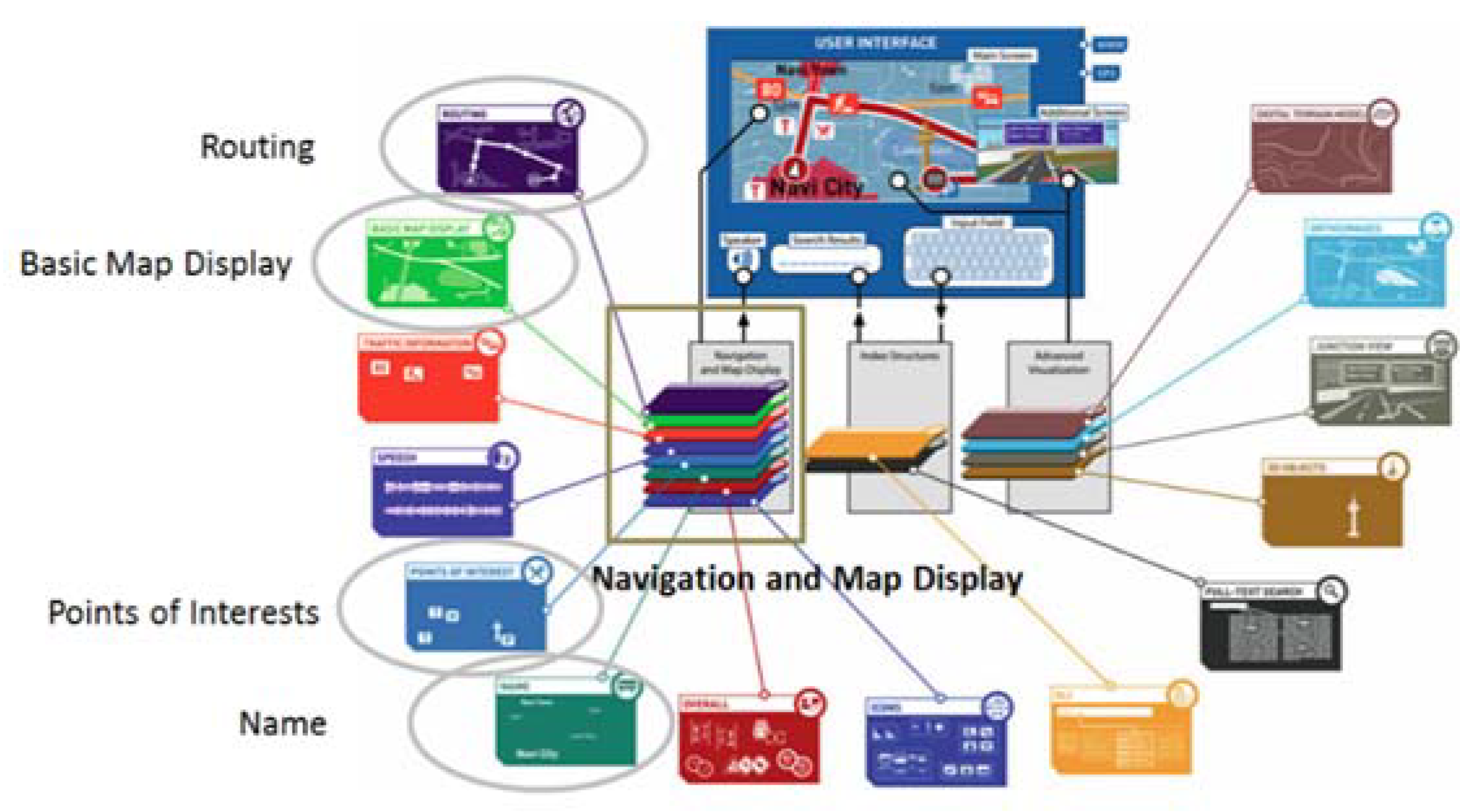
The NDS format is one of the global map standards developed by several automobile manufacturers, such as Daimler, BMW, Volkswagen Hyundai, application developers and map providers, such as Bosch, HERE and TomTom [18]. It is a standardized binary format whose typical advantages are e.g., incremental map updates and fast search capabilities in with databases using standardized parameters [18,20]. All data are assigned to the appropriate building block that addresses specific functional aspects of NDS (see Figure 1) in NDS format.
3.2. Basics of Map-Matching
Map-matching is a technique that integrates vehicle positioning data with digital road map data and is required to unambiguously identify the correct road link on which a vehicle is driving. By using orthogonal projection, the vehicle location on the matched road can be determined [22].
Map-matching technologies have become increasingly important in the last twenty years and there are numerous review articles as well as new developments on this topic [23,24,25,26,27,28,29]. In general, the map-matching algorithms can be classified into three categories: geometric, topological and attribute-based algorithms [1]. Geometric algorithms consider the geometric information of the digitalized points and lines. Typical geometric approaches are point-to-point matching, point-to-curve matching and curve-to-curve matching [30,31,32]. In topological algorithms the relationship between the features (points, lines and polygons) is taken into account. Typical relationships on the digital road maps are for example, the connectivity and contiguity of the road links, on which many map-matching algorithms are based [24,27,28,33,34]. In addition to geometric and topological information, the attributes on the digital road map can also be used to improve the reliability of map-matching algorithms. Typical attributes include the street name, travel direction, average speed, number of lanes, functional road classes, turn restrictions at the junction, etc. They can be used to avoid or correct incorrect matching of the vehicles [26,29,35,36,37,38,39,40]. Map-matching algorithms can be optimized by considering stochastic and decision-making methods (e.g., fuzzy logic [41], Dempster-Shafer theory, belief function theory).
In recent years, more and more lane-level map-matching algorithms have been developed based on HD maps [6,42,43]. The HD maps contain much more detailed and accurate information than the current navigation maps [15]. However, the new challenges are, for example, the real-time capability since a large amount of information needs to be considered and the topological connectivity information is not included in the lane-level map data and needs to be calculated in real-time [6].
3.3. Map-Matching Criteria and Total Weighting Score (TWS)
To identify the most probable candidate road link around the measured vehicle position (defined as an elliptical or rectangular confidence region around the vehicle), several criteria can be considered, such as the heading, closeness/proximity and connectivity. In [29], a weighting-function based map-matching algorithm was developed that considers all three similarity criteria: heading, closeness/proximity and connectivity. In this way, a so-called Total Weighting Score (TWS) can be calculated.
The candidate road link showing the highest TWS is determined to be the most likely candidate road link. The vehicle’s location is then matched with this road link.
However, this map-matching approach does not provide the solution for the TransSec project. Yet, it is the basic algorithm for the design of the map-aiding concept, therefore, and is therefore described below.
3.3.1. Map-Matching Criteria
The heading criterion describes the difference between the heading angles of the vehicle and a certain road link (after [24,28]), which can be expressed as a cosine function (see Equation (1)). Thus, the smaller the , the higher the weight will be:
where the difference between these two headings is defined as the angle between two 2D vectors and , one originating from the vehicle position and the other is from the road link:
In addition to the heading criterion, the proximity criterion depends on the distance between a point and a line in 2D, which is calculated as follows:
where (, ) are the coordinates of a measured vehicle position at epoch , the points (, ) and (, ) are the starting point and the endpoint of a road link , respectively.
The last criterion considered in the proposed algorithm is the link connectivity that is denoted as (after [24]):
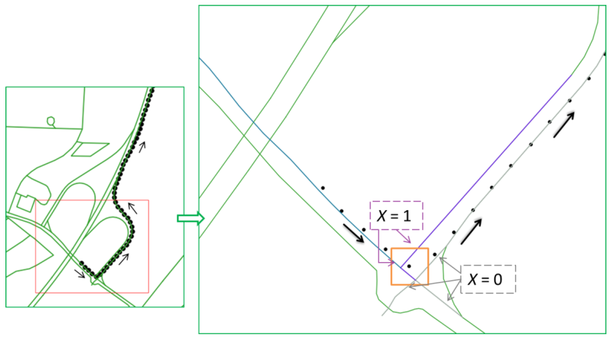
As illustrated in the Figure 2, the previously identified road link is marked in blue and the black dot in the orange square (the buffer zone) denotes the current vehicle position. For the road links connected to the blue link (marked in purple), the value is 1 (see Equation (4)); otherwise, there is no connectivity to the blue link, and is thus equal to 0. The road links with no connectivity to the previously identified link are marked in grey. This compensates for the shortcomings of geometric map-matching algorithms, which often fail because the connectivity between the current and the previously identified road link is not considered. Furthermore, the connectivity criterion in [24] is improved by comparing the length of the matched road link and the vehicle’s travel distance in one measuring epoch (e.g., 1 s) to reduce the percentage of mismatch in this work.
3.3.2. Total Weighting Score (TWS)
Since the heading angle of the first fixed vehicle position may be inaccurate, it is not used in the algorithm, so the map-matching process start with epoch number = 2. Using the abovementioned criteria, a weighting-function can be defined as (after [24,28]):
where the TWS for the measured vehicle position at epoch is determined from the weighting coefficients , and and the parameters , and related to heading, proximity and link connectivity criteria in Equations (2)–(4), respectively. The variable is used to define the buffer size (size of clipping window) for the search of the road link candidates. Since the second point of the vehicle trajectory has no previous matched road link, the coefficient is set to zero for = 2.
It has to be mentioned that the values of the weight coefficients , and are not predefinedand may depend on the operating environment. As stated in [24], either equal values or empirically determined values can be chosen for these coefficients. In the context of this work, it is convenient to assume the values in Equation (6) for , and :
Further details on this map-matching algorithm can be found in [29]. The accuracy of the measured vehicle position and the map are the essential factors for the performance of the map-matching algorithm. Inaccuracy of the measured vehicle position and the map may lead to incorrect results, i.e., means the most likely road link is not always correctly identified. Moreover, the variable is equal to half of the side length of the square buffer. According to the research results in [27], choosing an appropriate buffer size is not a simple matter, since it has a great impact on the map-matching result. These conditions lead to a complex adaption, integration and further development and research work.
4. Map-Supported Positioning
4.1. Data Availability and Quality Analysis
Different NDS versions have been analyzed. The lane-level geometry is defined in the latest version of the NDS format 2.5.X. However, no lane-level NDS map with a large coverage is available so far. Therefore, it was decided to use the latest available NDS map, which was Version 2.4.2 at the beginning of the project in 2018.
The map data availability of the NDS map Version 2.4.2 was investigated. The feature and attributes availability of TransSec use cases, such as pedestrian zones, shopping street and marketplaces as well as tourist promenades, were analyzed in details and the results are presented in [44] and it is not focus of this paper therefore it will not be shown again.
Furthermore, because the quality (especially the geometric accuracy) of map data is extremely important for the performance of the map-matching or map-aiding approaches, the quality of NDS map was analyzed. The results show that in the test area (total length of 147 km, mainly on non-motorway roads in urban areas, highway on-ramps and off-ramps and the German Autobahn), the absolute accuracy of the map is about 1.5 m and the relative accuracy is about 0.5 m [44].
4.2. Map-Aiding Approach
A map-matching algorithm is not a solution for the TransSec project, because it assumes that the truck is always on the road, so the algorithm “pulls” the truck’s position onto a road, so that it only detects the situation on the road. However, in the event of a terrorist attack, the driver could drive over road curbs, so that it is off the road, enter a prohibited or a restricted area, such as a pedestrian zone or a marketplace, or drive in the wrong direction. Consequently, a concept called map-aiding is being developed for the TransSec project.
The map-aiding approach detects areas where the truck should not travel and estimates deviations from the normal road course. The map-aiding approach can be considered as a modified and improved algorithm based on map-matching. It considers both on-road and off-road situations, detects wrong-way drivers, and provides the necessary information to identify whether the truck is potentially traveling in prohibited or restricted areas.
Another limitation of classical map-matching is that only one candidate road link is determined and displayed to the user. In the case of off-road situations, the truck may be located between two (or more) road links. If the TWS for two (or more) road links are quite similar, map-aiding should provide more than one road link. Therefore, map-aiding uses the most likely road link and other candidate road links in the defined buffer zone derived from map-matching as a baseline information. The principle of map-aiding can be divided into the following steps:
- (1)
- step 1: search for road candidate based on a well-defined weighting-function according to Equation (5) in Section 3.3.2,
- (2)
- step 2: identification of the road link with the highest TWS (reference link),
- (3)
- step 3: computation of the lateral position deviation d from the vehicle position to the identified road link (reference link),
- (4)
- Step 4: on-/off-road detection including a comparison of probability estimation (see Section 4.3),
- (5)
- step 5: identification of the lane on which the vehicle is travelling; wrong-way driver detection including probability estimation (see Section 4.4),
- (6)
- step 6: provide all necessary results (e.g., speed limit and direction of traffic flow, link type and number of lanes) of the reference link to identify potential risks.
Here it is essential to emphasize that map-aiding provides more additional information besides the identified road link with highest TWS. If more than one road links is located in the defined buffer zone, the associated results such as the calculated TWS, the coordinates of the start and end node of the road link, and the shortest distance for each link are stored additionally to identify potential risks.
Based on the above considerations, the main advantages of map-aiding compared to map-matching are highlighted as follows:
- (1)
- The identification on which lane the vehicle is actually traveling is added.
- (2)
- The probability estimation of the on-/off-road or the wrong-way driver is added.
- (3)
- Multiple road links are provided (if needed).
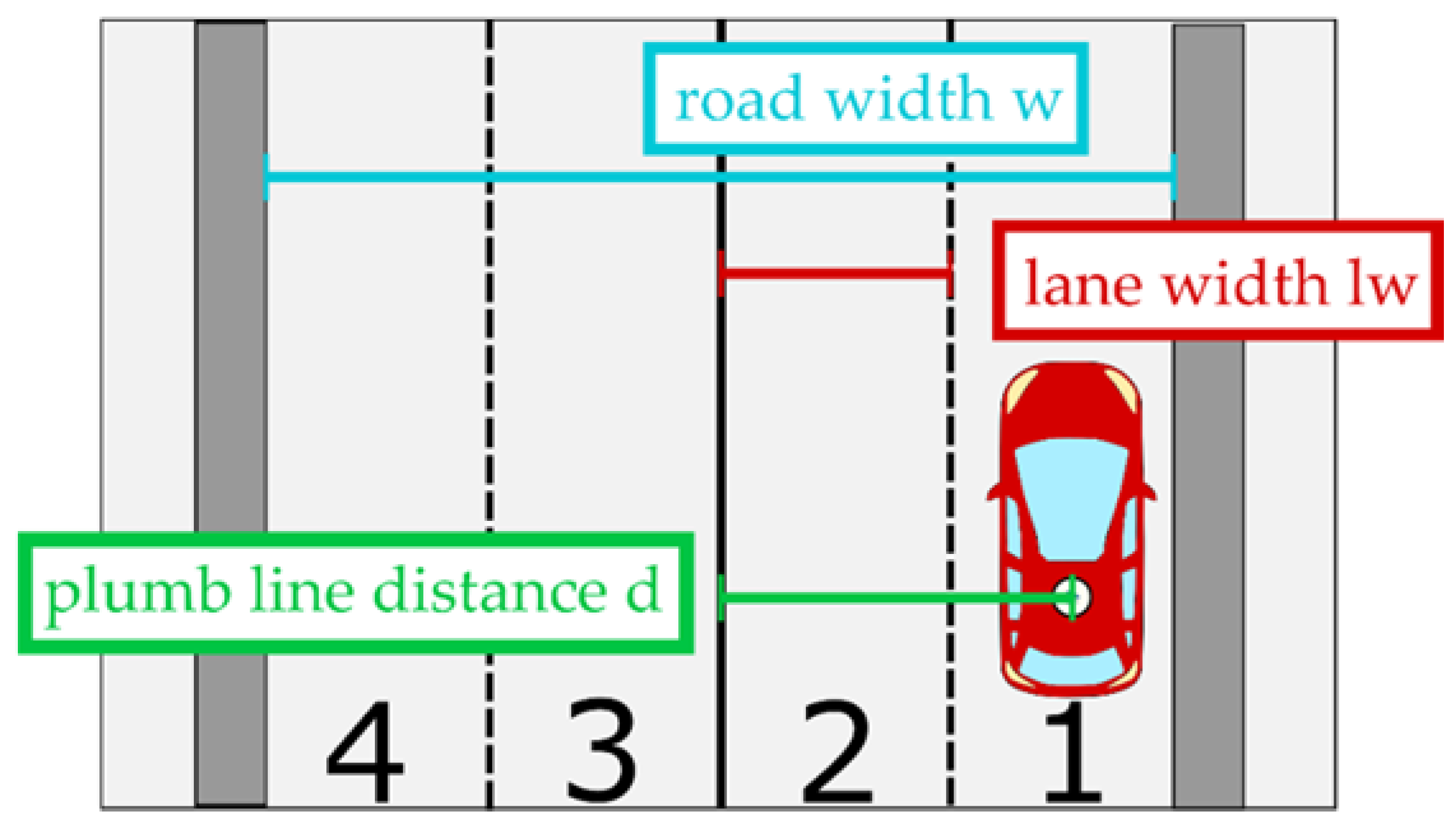
Since the actual road width is not available, it has to be derived from the number of lanes. As mentioned beforehand, the NDS map database (version 2.4.2) used in the TransSec project is at road-level, in which no lane geometry is included. For example, a multi-lane road is modeled as one single polyline representing the road center line. However, the attribute “the number of lanes” is available for most roads, but no exact value of road width or lane with is assigned to each individual road link. Thus, the implemented lane identification within the map-aiding is based on the assumption that the lane generally keeps an approximately constant width of 3.50 m. This default value can be found in the region metadata table of Overall Building Block in NDS data.
4.3. On-/Off-Road Detection including Probability Estimation
In the case of terrorist attacks, the vehicle could drive over the road curb so that it is off-road; therefore, the off-road situation needs to be detected and the probability needs to be calculated.
Figure 3 gives an example of a four-lane road to illustrate how an on-/off-road decision based on the number of lanes can be done.
The basic idea of on-/off-road detection is to compare the plumb line distance of the vehicle from the center of the road and half width of road , their difference can be calculated as:
where the road width can be calculated by the lane width and the number of lanes from the map data:
Generally, from a statistical point of view, a significance test is performed to check whether is significantly larger or smaller than zero:
For the probability estimation, the standard deviation of needs to be calculated, for this purpose the standard deviations of and (,) are required.
The standard deviation of the plumb line distance can be obtained by variance propagation from the Equations (3), and the associated variances as follows:
where is the Jacobian matrix of Equation (3) and is its associated covariance matrix. is the standard deviation of the map. Here, it represents the average deviation of the map from the true reference. is set based on empirical investigations in [44] and was divided equally between X- and Y-direction, it means .
is the standard deviation of the vehicle position. Either this can be taken dynamically from the position determination with each new time step or, if this is not possible, it can be determined as a static value. In the simulation in Section 5.1.2 different values are set. If no separate standard deviation for X- and Y-direction is available, a uniform distribution is assumed here as well.
The standard deviation of the road width can be calculated by equation based on Equation (8) and variance propagation:
where is the standard deviation of the lane width. For the test area, an average value of could be determined based on a random sampling of .
The standard deviation can now also be determined by applying the variance propagation to the Equation (7) as follows:
For deciding if or in Equation (8), the test quantity needs to be determined as follows:
It is assumed that follows the standard normal distribution, with the help of the respectively the according probability can be calculated [45]. For example, if the vehicle deviates 2.5 m off the road () and a standard deviation of can be calculated, this results in a test statistic of and thus a probability of that an off-road case exists.
4.4. Wrong-Way Driver Detection including Probability Estimation
In the event of a terror attack, a vehicle may travel in the direction opposite to the permitted direction of travel established for this road link. Therefore, the wrong-way driver must be detected and its probability must also be calculated.
Roads have three options for regulating traffic. They can be open for traffic in one, two or no direction. On the map, the object attributes correspond to one-way, two-way or closed. For roads with the attribute closed, a wrong-way driver can be directly assumed. More detailed investigations are required for the other two possibilities, and the procedure for doing so is described in Section 4.4.1 and Section 4.4.2. In Section 4.4.3 it is explained, when the wrong-way driver alert is sent.
4.4.1. Road Link with Attribute “One-Way”
If the attribute “one-way” is appropriate, the permitted direction of travel can be directly and unambiguously determined from the geometry and attribute of the road link. The geometry, more precisely the start and end point of the road link, determines the direction of the road. However, this does not have to correspond to the permitted direction of travel. Whether it corresponds to this is stored as its attribute. The wrong-way driver check decision is based on a comparison of the angle between the trajectory of the vehicle and the road link . When driving in the correct direction, the two angles differ only slightly. In case of a wrong direction of travel, they differ significantly. In Equations (16) and (17) the angles are calculated as follows:
where (, ) and (, ) are the coordinates of a measured vehicle position at epoch and − 1 respectively, the points (, ) and (, ) are the starting point and the endpoint of a road link , respectively.
With the angles calculated this way and the associated standard deviations (, a significance test is performed to check whether they differ significantly. If so, a wrong-way driver is assumed. The standard deviations depend on the prevailing geometry and therefore have to be recalculated at every time step. This is carried out by variance propagation from the standard deviation of the map and the position of the vehicle . For example, the calculation of is based on Equations (18)–(20). The calculation of can be calculated in a similar way by the variance propagation using the standard deviation of the vehicle position :
4.4.2. Road Link with Attribute “Two-Way”
If the attribution “two-way” is appropriate, it is not possible to infer the allowed direction of travel from the orientation of the road link, because both directions of travel are allowed. In countries with right-hand traffic, however it can be assumed, that the direction of travel to the right of the center is positive and to the left negative. In other words, a vehicle must always be right of the centerline following its own direction of travel. The middle of the road is used here as the separation between the lanes. However, this is not optimal, because for road links with an odd number of lanes, the center of the road lies within the middle lane. Therefore, no statement can be made for this lane, since more detailed information are missing.
Case: Even Number of Lanes
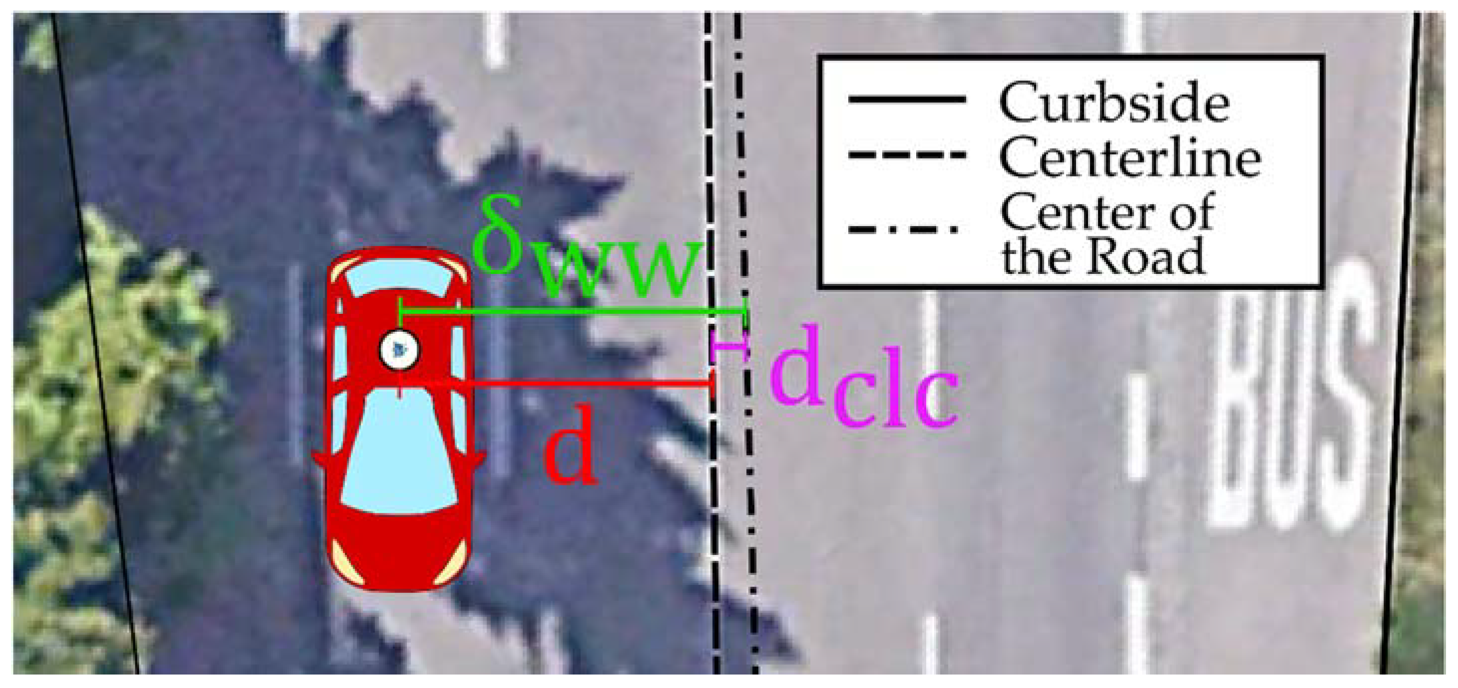
For an even number of lanes, it can be assumed that the center represents the separation between the two directions of travel. Thus, the position of the vehicle, left or right of the centerline in the direction of travel can be used to determine whether it is traveling in the correct direction. In other words, a significance test is applied to decide whether the position of the vehicle is to the left or to the right of the center of the road. For this purpose, it is first checked whether the vehicle is significantly away from the center line. Thus, it is tested whether the distance is significantly different from zero, with or . In reality, the geometrical center of the road may not correspond with the line separating the two directions of travel (see Figure 4). This distance is called . An expected value (mean) of zero is assumed over the entire map, since values cancel each other out due to the different signs depending on the direction of travel. The actual differences are thus described by their standard deviation, in which the improvements are quadratic, therefore independent of the sign. This was determined at , based on a random sampling of in the test area. The distance to the center line and its standard deviation are thus calculated as follows:
For deciding if or the test is performed analog to Section 4.3. If it is determined that the vehicle position is different from that of the centerline, a determinant test can be used to determine whether the vehicle is to the left or to the right of the centerline. For this purpose, the auxiliary matrix is set up and then its determinant is determined:
The determinant can take three values (), where is excluded by the preceding test. For , the vehicle is on the right and thus correct side of the centerline. For it’s on the left side, indicating that the driver is the wrong way round.
Case: Odd Number of Lanes
If there is an odd number of lanes, this statement can only be made for all lanes except the middle one, as mentioned above. To ensure that the vehicle is not in the middle lane, it is checked whether the vehicle is significantly more than half a lane width from the centerline. This can also be expressed by the difference , which is larger than zero for all lanes except the middle one:
For deciding if or the test is performed analog to Section 4.3. If it is determined that the vehicle is on another lane than the middle one, a determinant test (analog to the procedure with an even number of lanes) is performed to decide for the driving direction.
4.4.3. Wrong-Way Driver Alert
Due to different influences, which will be explained in more detail in Section 5.3, false alarms occur during the wrong-way driver detection. To reduce these, an alarm is only issued if at least three consecutive, different positions have triggered a wrong-way driver message. By doing so, the rate of false alarms could be reduced by about 60%. However, the reaction time is extended by two seconds, at a GNSS data rate of 1 Hz, which was considered to be acceptable.
5. Evaluation
5.1. Test Scenario
5.1.1. Real Trajectories
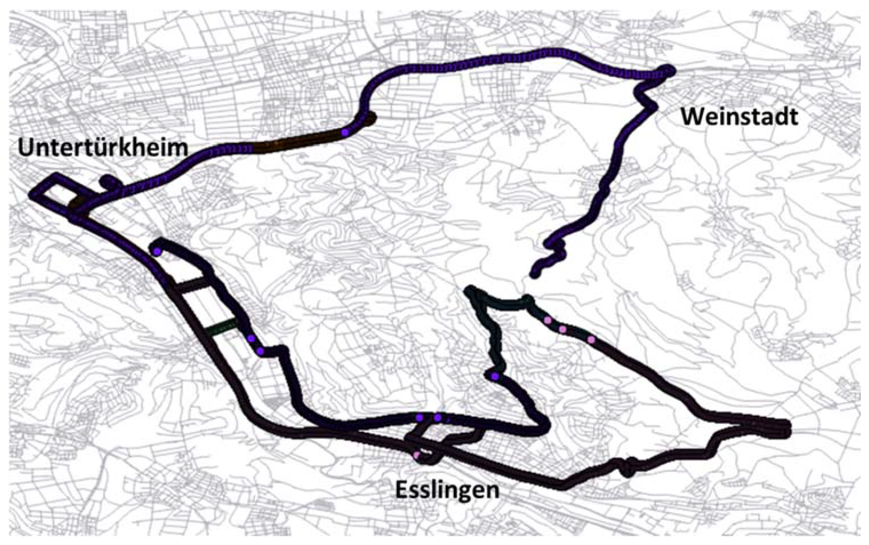
Comprehensive test drives are carried out in the vicinity of Stuttgart Untertürkheim, Esslingen and Weinstadt with a total distance of approx. 55.1 km. The trajectories contain 27,452 vehicle positions and 430 number of road links, they are presented in Figure 5. For the test drives carried out by the project partner Daimler, different geodetic-grade/high-end GNSS receivers are applied for performance evaluation. One of them is the BX982 GNSS receiver provided by the company Trimble [46]. The multi-channel and multi-frequency Trimble BX982 has a dual antenna input and is capable to achieve centimeter-level accuracy and heading [46]. The positioning accuracy obtained with GNSS depends to a large extent on the environmental conditions and the mode of operation [47].
5.1.2. Simulated Trajectories
In addition to the real data, simulated data was also used for evaluation. With these simulated data, larger data sets could be generated with reasonable effort, and trajectories could be created that included driving maneuvers, such as wrong-way driving, which could not have been recorded in real traffic.
For this purpose, “nominal trajectories” were first generated, to which an error was added. By generating the ”nominal trajectories” first, they could be used for the evaluation of the map-aiding results. In addition, the comparability of the individual trajectories could be guaranteed. Since they describe the same driving maneuver in the origin and differ only in their simulated errors.
To generate the nominal trajectories, an algorithm has been developed that generates random routes based on a digital road map and the attributes contained therein. At the beginning, the generator randomly selects a road edge and determines an initial direction. This initial direction represents the direction of travel. In this direction, the algorithm searches for the next intersection and stores all road edges that are “traveled” up to this intersection. At the intersection, a random decision is made in which direction to continue the “driving”. Thus a sequence of individual road edges is created. The exact positions are then interpolated between the start and end points of the individual road edges. The number of these positions depends on the length of the segment and the maximum speed allowed in each case. In this way, for example, wrong-way drivers can also be simulated, e.g., by turning into a one-way street against the permitted direction of travel at an intersection. Since the maximum speed is always assumed, traffic lights, stop signs and traffic, for example, are not taken into account. Also, all roads are driven on with the same probability and thus similar frequency. Thus, contrary to reality, main roads do not occur more frequently in the trajectories than secondary roads.
A typical behavior of GNSS trajectories, especially in urban environments, is a parallel offset of the trajectory section [48,49]. To consider such systematics, which can be caused e.g., by the geometric constellation or multipath effects [50] the “nominal trajectories” are adjusted by applying a systematic error and a random error [51]. The root mean square of the measurement deviations is used as a parameter for the assessment of systematic and random error [52]:
where is constant for one simulation run. In the evaluations, the values 0.5, 1 and 2 m were chosen. The ratio between and is chosen randomly, but is constant for a road link ().
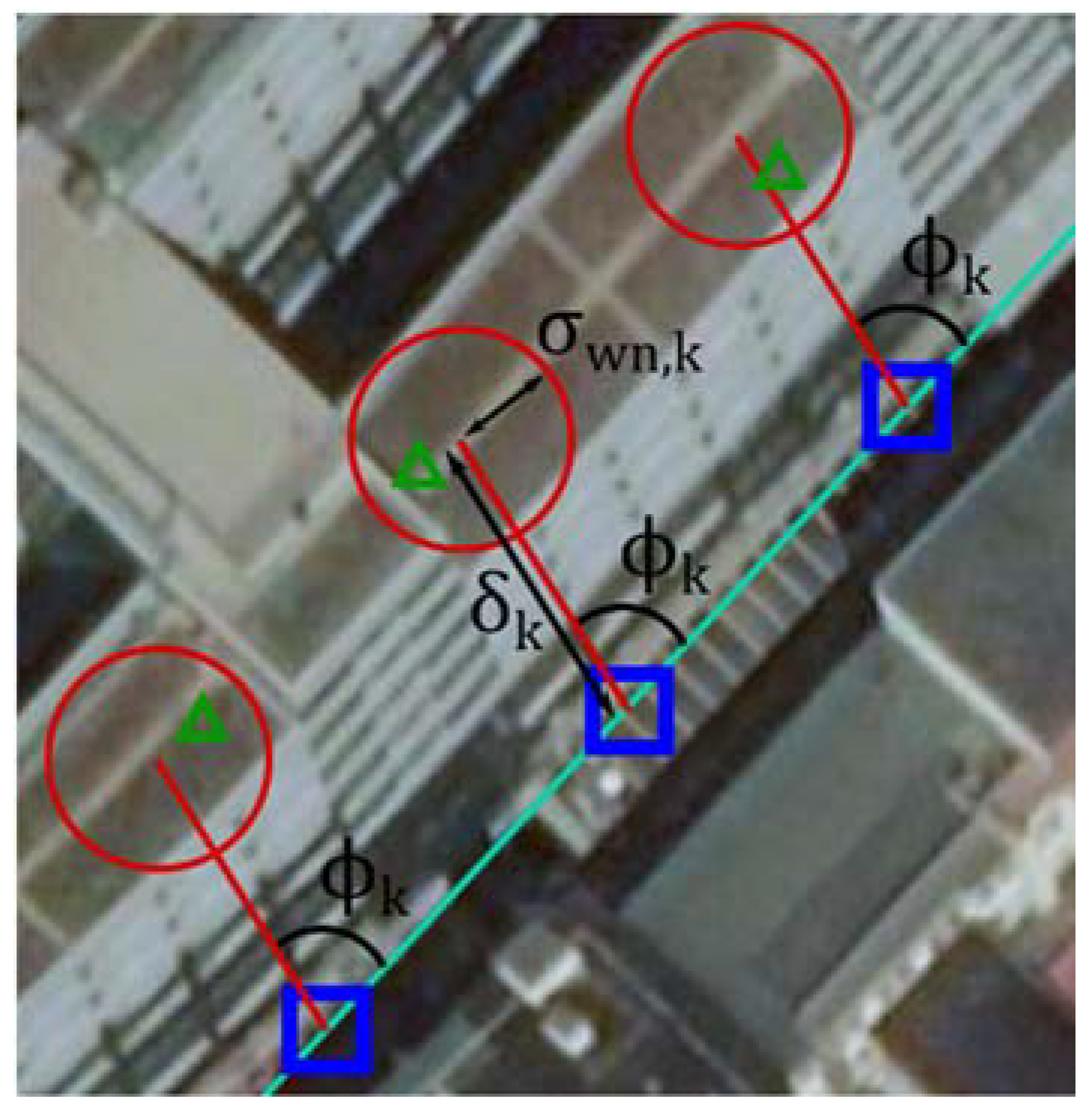
The systematic error is described by two parameters. The first parameter indicates the size of the error () and the second the direction of the error, which is selected randomly, but is fixed for a complete road link (see Figure 6):
The random error is represented by a multivariate normal distribution , with the expected value and the covariance matrix , which contains the standard deviation divided in X- and Y-direction ():
In order to assign a point of a nominal trajectory with both, the systematic and the random error, the systematic error (cf. Equation (28)) is applied first. The result is then taken as the expected value of the normal distribution (cf. Equation (29)). Thus, the following model is obtained for a point with simulated error :
In total, “target trajectories” with an approximate total length of 1980.4 km were generated. These are distributed as shown in Table 1.
5.2. Results
In the following, the numerical results, divided into simulated and real trajectories, are shown.
5.2.1. Results of Real Trajectories
Since the test drive is in an urban environment, the truck is always traveling on the road and there are no off-road or wrong-way driver scenarios. The real trajectories can be used to investigate the performance of the map-aiding algorithms for on-road scenarios in a complex urban road network.
Table 2 and Table 3 present the confusion matrix of off-road and wrong-way driver detection for real trajectories respectively. Since the real trajectories do not contain any off-road or wrong-way driver parts, only the specificity or false positive rate can be analyzed. For the false positive rate, a value of respectively was achieved. This means, that the developed map-aiding approach performs quite well even at complex road conditions such as road intersections, junctions, overpasses and underpasses. The results are quite satisfying, since the density and complexity of road network in urban areas is much higher than that in rural areas and on highways, the proposed map-aiding approach pays special attention to urban areas where map-aiding can be particularly challenging. Mostly, the map-aiding approach delivers correct results for on/off-road estimation and lane identification although the road geometry (e.g., of intersections) on the digital road map database is strongly simplified or the vehicle positions are very inaccurate.
5.2.2. Results of Simulated Trajectories
Therefore, for a complete evaluation of the detection rate, the simulated trajectories have to be used, which also include simulated prohibited driving maneuvers. Table 4 and Table 5 show the confusion matrix of off-road and wrong-way driver detection for simulated trajectories with different measurement deviations = 0.5, 1 and 2 m.
As shown in Table 6, the false positive rate is in a similar range of values as for the real trajectories in Section 5.2.1. Therefore, it can be assumed that the simulated trajectories are well suited for the evaluation of the algorithm.
From the off-road detection result, it can be seen that the false positive rate decreases as the position accuracy increases, so that the position accuracy correlates with the false alarms rate. This correlation cannot be seen for the wrong-way driver detection. There, a limited growth is shown, which, on the other hand, is accompanied by a decreasing sensitivity. This can be explained by the fact that here the significance of the results is rejected more often, which leads to more omitted alarms. The wrong-way driver detection works well for both common and structurally separated lanes. Due to the larger tolerances that occur when a lane can only be used in one direction (separated lane or one-way street) the results are better.
5.3. Analysis
In general, the map-aiding approach works well. Its performance depends on two main factors. On the one hand on the accuracy of the vehicle position, on the other hand on how much the road differs in reality from the assumptions that are defined (map accuracy).
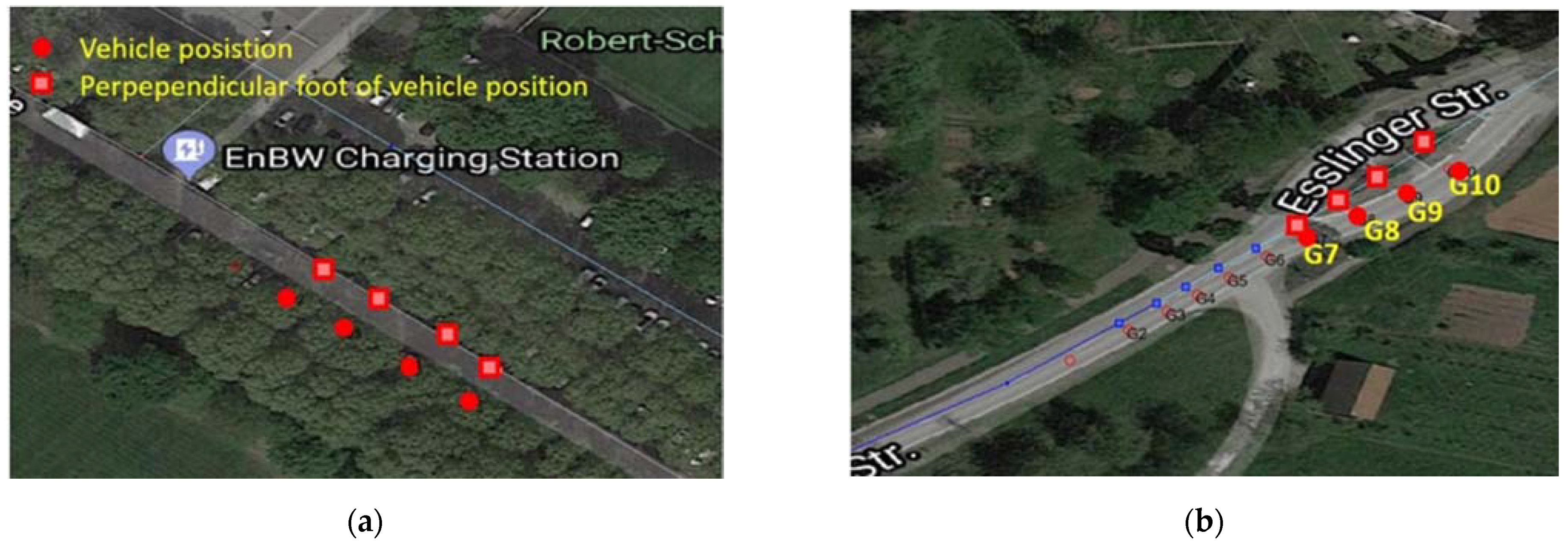
Figure 7a is an example within the real trajectories introduced in Section 5.1.1. It gives an impression of common environmental conditions in urban areas in which the view of the sky is partially blocked by trees along both sides of the road. Therefore, the position from the GNSS is very inaccurate (the error due to multipath effect could be several meters). Although the reference link is correctly identified, the estimated positional deviation from the inaccurate vehicle position to the reference link is 7.22 m, larger than the half width of a two-lane road (3.5 m). The vehicle position is identified as off-road with a probability of 99.99% and an off-road distance of 3.72 m. The perpendicular foot of the off-road vehicle position on the identified reference link is represented by a light red rectangle symbol. In this challenging scenario, the integration of sensors instead of GNSS-only could be helpful.
Figure 7b represents another example with incorrect off-road estimation due to inaccuracies in the road map data. At approximately vehicle position G7 the two lanes of the road “Esslinger Straße” are separated by a grass median strip. This real-world road geometry is not considered in the road map data. This directly leads to the incorrect off-road estimation for vehicle positions G8 to G10, although the vehicle is actually on the road. In this challenging scenario, object detection based on camera and lidar or HD maps is essential to avoid false alarms.
In general, there are three factors for the inaccuracy of the map data. First, the assumption that the centerline representing the road on the map is the same than the center of the road in reality. However, this is not always the case, and individual roads can be much less accurate. In fact, this is usually a displacement of the complete street perpendicular to it. Depending on the sign of the displacement, this can result in both, omitted alarms and false alarms. This factor was considered with the standard deviation and in the developed approach. Secondly, the assumption that a lane is 3.50 m wide. In reality, roads deviate from this assumption for different reasons. This factor was taken into account with the standard deviation and respectively. These two factors of map data inaccuracies are described with the associated standard deviations, but each with only one standard deviation for the entire map. Therefore, individual roads can be significantly less accurate. The third factor is the geometrical conformity. Sometimes a road or the traffic routing does not run as shown on the map. This can be caused through temporary changes in the traffic flow or permitted driving maneuvers on the oncoming lane, such as overtaking maneuvers or when turning off, but also through errors in the generation of the digital map (as already shown as example in Figure 7b).
6. Conclusions and Outlook
In this paper, the one lane-level map-aiding approach based on non-lane-level NDS map was introduced, it was developed within the TransSec project for prevent the terror attacks using trucks. The developed map-aiding approach is based on the map-matching algorithm. Classical map-matching algorithms assume that the respective road user obeys the traffic rules. For the classical application in navigation, this assumption is also correct and can be used for the support of the positioning. From the point of view transport safety however, this the only “on-road” scenario and obedience of the traffic rules and cannot be assumed. In order to recognize a possible dangerous situation, all possibilities have to be considered. Therefore, a lane-level map-aiding approach has some advantages or additional functions. The identification of lane, on which the vehicle is travelling is possible; the probabilities of on-/off-road and wrong-way driver are calculated for risk estimation; the multiple road links can be provided; for the associated map attributes like travel direction, speed limits are provided for detecting potential risks. The additional functions make the wide application of developed lane-level map-aiding approach possible such as lane support systems and wrong-way driver detections (see Section 2.1). Of course, the developed map-aiding approach is not limited to the intended application within the TransSec project for the trucks, it can be applied for other lane-level localization of other vehicles.
The highlight and innovation of the developed map-aiding approach is the probability estimation for on-/off-road and wrong-way driver for risk estimation. The developed map-aiding approach was evaluated comprehensively with the real and simulated trajectories. False positive rates are less than 1.3% for on-/off-road and wrong-way driver detection, and the sensitives are better than 99.1% for off-road and wrong-way driver detection. It means the developed map-aiding approach works quite robust. in combination with object detection based on-board cameras and lid ar sensors, false results of potential risk could be reduced.
The false results are due to the inaccuracies of the vehicle position and the map. The performance of map-aiding approach could even better with more accurate vehicle position and HD maps in the near future. The map-aiding approach could be adapted to the lane-level HD maps. More accurate map data is available in lane-level HD maps, and it means less standard deviations of map data can be used for probability estimation. The multisensor system could provide the more accurate and reliable vehicle positions for probability estimation. The simulations show, in general, the accurate the position is the better is the result of probability estimation results of the map-aiding approach.
As a summary, the developed map-aiding approach could be adopted using HD map and a highly accurate positioning system for the road transport safety and security application with even better performance in the near future. The developed map-aiding approach is not limited to the non-lane-level map and application for risk estimation for terror attacks using trucks, it could be used for many other applications and its significance and huge potential cannot be underestimated in road transport safety and security.
Author Contributions
Map-matching and map-aiding (part: on-/off-road estimation) is developed and implemented by J.W. Map-Aiding (part: wrong-way driver detection) and probability estimation was developed and implemented by P.L. The original draft of Section 3, Section 4.1, Section 4.2 and Section 5.1.1 were prepared by J.W. and edited by L.Z. Section 1, Section 2 and Section 6 were written by L.Z. Section 4.3, Section 4.4, Section 5.1.2, Section 5.2 and Section 5.3 were written by P.L. and edited by L.Z. The TransSec project was supervised by V.S. and paper was reviewed by V.S. All authors have read and agreed to the published version of the manuscript.
Funding
The investigations published in this article are granted by GSA (European GNSS Agency) within the H2020-GALILEO-GSA-2017 Innovation Action with Grant Agreement Nr.:776355 and by the German Federal Ministry of Economic Affairs and Energy (BMWi) and the German Aerospace Center (DLR) under grant number 50 NA 1802.
Institutional Review Board Statement
Not applicable.
Informed Consent Statement
Not applicable.
Data Availability Statement
Data available from the corresponding author upon request.
Conflicts of Interest
The authors declare no conflict of interest.
References
- Wang, J.; Wachsmuth, M.; Metzner, M.; Schwieger, V. Die digitale Karte als Sensor. In MST 2018—Multisensortechnologie: Low-Cost Sensoren im Verbund: Proceedings of the 176. DVW-Seminar, Hamburg, Germany, 13–14 September 2018; Wißner Verlag: Augsburg, Germany, 2018; pp. 137–166. [Google Scholar]
- Kim, K.; Seol, S.; Kong, S. High-speed train navigation system based on multi-sensor data fusion and map matching algorithm. Int. J. Control Autom. Syst. 2015, 13, 503–512. [Google Scholar] [CrossRef]
- Wang, P.; Li, W.; Wang, X.; Chu, X. The Method of Train Positioning Based on Digital Track Map Matching. MATEC Web Conf. 2018, 246, 03024. [Google Scholar] [CrossRef]
- Safe Road Transport Roadmap towards Vision Zero: Roads without Victims. ERTRAC Working Group: Road Transport Safety & Security. Available online: https://www.ertrac.org/uploads/documentsearch/id58/ERTRAC-Road-Safety-Roadmap-2019.pdf (accessed on 29 July 2021).
- Pappalardo, G.; Cafiso, S.; Di Graziano, A.; Severino, A. Decision Tree Method to Analyze the Performance of Lane Support Systems. Sustainability 2021, 13, 846. [Google Scholar] [CrossRef]
- Luz, P.; Metzner, M.; Schwieger, V. Development of a new lane-precise map matching algorithm using GNSS considering road connectivity. In Proceedings of the Virtual ITS European Congress 2020, Online, 9–10 November 2020. [Google Scholar]
- Nice Truck Attack. Available online: https://en.wikipedia.org/wiki/2016_Nice_truck_attack (accessed on 30 July 2021).
- Berlin Truck Attack. Available online: https://en.wikipedia.org/wiki/2016_Berlin_truck_attack (accessed on 30 July 2021).
- Vehicle-Ramming Attack. Available online: https://en.wikipedia.org/wiki/Vehicle-ramming_attack (accessed on 30 July 2021).
- TransSec Website. Available online: http://www.transsec.eu/ (accessed on 23 July 2020).
- TransSec Deliverable D2.1 Requirements for Positioning Quality. Available online: http://www.transsec.eu/public-deliverables/ (accessed on 6 January 2020).
- Wachsmuth, M.; Koppert, A.; Zhang, L.; Schwieger, V. Development of an error-state Kalman Filter for Emergency Maneuvering of Trucks. In Proceedings of the European Navigation Conference, Online, 23–24 November 2020. [Google Scholar]
- ISO. ISO/TR 17424. ISO/TR 17424:2015 Intelligent Transport Systems—Cooperative Systems—State of the Art of Local Dynamic Maps Concepts; ISO: Geneva, Switzerland, 2015. [Google Scholar]
- Eskandarian, A. Handbook of Intelligent Vehicles, 1st ed.; Springer: London, UK, 2012; Volume 2. [Google Scholar]
- Liu, R.; Wang, J.; Zhang, B. High Definition Map for Automated Driving: Overview and Analysis. J. Navig. 2020, 73, 324–341. [Google Scholar] [CrossRef]
- Ehmke, J. Integration of Information and Optimization Models for Routing in City Logistics, 1st ed.; Springer: New York, NY, USA, 2012. [Google Scholar]
- ISO. ISO 20524-1:2020 Intelligent Transport Systems—Geographic Data Files (GDF) GDF5.1—Part 1: Application Independent Map Data Shared between Multiple Sources; ISO: Geneva, Switzerland, 2020. [Google Scholar]
- NDS Website. Available online: https://nds-association.org/ (accessed on 6 April 2021).
- OpenDRIVE Website. Available online: https://www.asam.net/standards/detail/opendrive/ (accessed on 6 April 2021).
- Kleine-Besten, T.; Behres, R.; Pöchmüller, W.; Engelsberg, A. Digital Maps for ADAS. In Handbook of Driver Assistance Systems, 1st ed.; Winner, H., Hakuli, S., Lotz, F., Singer, C., Eds.; Springer International Publishing: Basel, Switzerland, 2016; Volume 26. [Google Scholar]
- NDS Version 2.4.2. Navigation Data Standard Format Specification, NDS Version 2.4.2; NDS e.V.: Gries, Germany, 2015. [Google Scholar]
- Beckmann, H.; Frankl, K.; Wang, J.; Metzner, M.; Schwieger, V.; Eissfeller, B. Real-world vehicle tests for determining the minimum time of detection for wrong-way driving on highways. In Proceedings of the Navitec Conference, Noordwijk, The Netherlands, 14–16 December 2016. [Google Scholar]
- Quddus, M.; Ochieng, W.Y.; Noland, R.B. Current Map-Matching algorithms for transport applications: State-of-the art and future research directions. Transp. Res. Part C Emerg. Technol. 2007, 15, 312–328. [Google Scholar] [CrossRef] [Green Version]
- Velaga, N.; Quddus, M.; Bristow, A. Developing an enhanced weight-based topological Map-Matching algorithm for intelligent transport systems. Transp. Res. Part C Emerg. Technol. 2009, 17, 672–683. [Google Scholar] [CrossRef] [Green Version]
- Velaga, N.; Quddus, M.; Bristow, A. Detecting and Correcting Map-Matching Errors in Location-Based Intelligent Transport Systems. In Proceedings of the 12th World Conference on Transport Research, Lisbon, Portugal, 11–15 July 2010. [Google Scholar]
- Abdallah, F.; Nassreddine, G.; Denoeux, T. A multiple-hypotheses map matching method suitable for weighted and box-shaped state estimation for localization. IEEE Trans. Intell. Transp. Syst. Symp. 2011, 12, 1495–1510. [Google Scholar] [CrossRef]
- Blazquez, C. A Decision-Rule Topological Map-Matching Algorithm with Multiple Spatial Data. In Global Navigation Satellite Systems: Signal, Theory and Applications, 1st ed.; Shuanggen, J., Ed.; InTechOpen: London, UK, 2012; pp. 215–240. [Google Scholar]
- Quddus, M.; Washington, S. Shortest path and vehicle trajectory aided Map-Matching for low frequency GPS data. Transp. Res. Part C Emerg. Technol. 2015, 55, 328–339. [Google Scholar] [CrossRef] [Green Version]
- Wang, J.; Metzner, M.; Schwieger, V. Weighting-function based Map-Matching algorithm for a reliable wrong-way driving detection. In Proceedings of the 12th ITS European Congress, Strasbourg, France, 19–22 June 2017. [Google Scholar]
- Bernstein, D.; Kornhauser, A. An Introduction to Map Matching for Personal Navigation Assistants; New Jersey TIDE Center, Princeton University: Newark, NJ, USA, 1996. [Google Scholar]
- Czommer, R. Leistungsfähigkeit Fahrzeugautonomer Ortungsverfahren auf der Basis von Map-Matching-Techniken. Ph.D. Thesis, University of Stuttgart, Stuttgart, Germany, 2000. [Google Scholar]
- Röhrig, C.; Büchter, H.; Kirsch, C. Monte Carlo Lokalisierung Fahrerloser Transportfahrzeuge mit drahtlosen Sensornetzwerken. In Autonome Mobile Systeme 2009, 1st ed.; Dillmann, R., Beyerer, J., Stiller, C., Zöllner, J.M., Gindele, T., Eds.; Springer: Berlin/Heidelberg, Germany, 2009; pp. 161–168. [Google Scholar] [CrossRef]
- Ochieng, W.Y.; Quddus, M.A.; Noland, R.B. Map-Matching in complex urban road networks. Braz. J. Cartogr. 2003, 55, 1–18. [Google Scholar]
- Hashemi, M.; Karimi, H.A. A weight-based map-matching algorithm for vehicle navigation in complex urban networks. J. Intell. Transp. Syst. 2016, 20, 573–590. [Google Scholar] [CrossRef]
- Krumm, J.; Letchner, J.; Horvitz, E. Map Matching with Travel Time Constraints. Available online: www.microsoft.com/en-us/research/publication/Map-Matching-travel-time-constraints (accessed on 14 April 2021).
- Kuhnt, F.; Kohlhaas, R.; Jordan, R.; Gußner, T.; Gumpp, T.; Schamm, T.; Zöllner, J.M. Particle filter map matching and trajectory prediction using a spline based intersection model. In Proceedings of the 17th International IEEE Conference on Intelligent Transportation Systems (ITSC), Qingdao, China, 8–11 October 2014; pp. 1892–1893. [Google Scholar] [CrossRef]
- Luo, A.; Chen, S.; Xv, B. Enhanced Map-Matching Algorithm with a Hidden Markov Model for Mobile Phone Positioning. ISPRS Int. J. Geo Inf. 2017, 6, 327. [Google Scholar] [CrossRef] [Green Version]
- Li, F.; Bonnifait, P.; Ibanez-Guzman, J.; Zinoune, C. Lane-level Map-Matching with integrity on high-definition maps. In Proceedings of the IEEE Intelligent Vehicle Symposium (IV2017), Los Angeles, CA, USA, 11–14 June 2017; pp. 1176–1181. [Google Scholar]
- Heidrich, W.A.; Schulze, M.; Kessel, M.; Werner, M. Robustes Mapmatching Hochaufgelöster, Fahrzeugbasierter GPS-Tracks. Available online: www.martinwerner.de/pdf/MAPMATCH.pdf (accessed on 14 April 2021).
- Romon, S.; Bressaud, X.; Lassarre, S.; Pierre, G.S.; Khoudour, L. Map-Matching Algorithm for Large Databases. J. Navig. 2015, 68, 971–988. [Google Scholar] [CrossRef] [Green Version]
- Tang, J.; Zhang, S.; Zou, Y.; Liu, F. An Adaptive Map-Matching Algorithm Based on Hierarchical Fuzzy System from Vehicular GPS Data. Available online: http://journals.plos.org/plosone/article?id=10.1371/journal.pone.0188796 (accessed on 14 April 2021).
- Rabe, J.; Meinke, M.; Necker, M.; Stiller, C. Lane-level Map-Matching based on optimization. In Proceedings of the 2016 IEEE 19th International Conference on Intelligent Transportation Systems (ITSC), Rio de Janeiro, Brazil, 1–4 November 2016; pp. 1155–1160. [Google Scholar] [CrossRef]
- Sharath, M.; Velaga, N.R.; Quddus, M.A. A dynamic two-dimensional (D2D) weight-based Map-Matching algorithm. Transp. Res. Part C Emerg. Technol. 2019, 98, 409–432. [Google Scholar] [CrossRef]
- Zhang, L.; Wang, J.; Wachsmuth, M.; Gasparac, M.; Trauter, R.; Schwieger, V. Role of Digital Maps in Road Transport Security. In Proceedings of the FIG Working Week 2019, Hanoi, Vietnam, 22–26 April 2019. [Google Scholar]
- Rooch, A. Statistik für Ingenieure: Wahrscheinlichkeitsrechnung und Datenauswertung Endlich Verständlich, 1st ed.; Springer: Berlin/Heidelberg, Germany, 2014. [Google Scholar] [CrossRef]
- Trimble BX982. Available online: https://oemgnss.trimble.com/product/trimble-bx982/ (accessed on 10 April 2021).
- TransSec. Deliverable 3.4: Map Aiding. Project TransSec, WP3; Confidential Project Report; University of Stuttgart: Stuttgart, Germany, 2020. [Google Scholar]
- Ramm, K.; Schwieger, V. Multisensorortung für Kraftfahrzeuge. In Kinematische Messmethoden—Vermessung in Bewegung: Proceedings of the 58. DVW-Seminar, Stuttgart, Germany, 17–18 February 2004; Wißner Verlag: Augsburg, Germany, 2004. [Google Scholar]
- Eichhorn, E. Ein Beitrag zur Identifikation von Dynamischen Strukturmodellen mit Methoden der Adaptiven Kalman-Filterung. Ph.D. Thesis, University of Stuttgart, Stuttgart, Germany, 2000. [Google Scholar]
- Zhang, L.; Schwieger, V. Reducing multipath effect of low-cost GNSS receivers for monitoring by considering temporal correlations. J. Appl. Geod. 2014, 14, 167–175. [Google Scholar] [CrossRef]
- Niemeier, W. Ausgleichungsrechnung: Statistische Auswertemethoden, 2nd ed.; de Gruyter: Berlin, Germany, 2008. [Google Scholar]
- Sachs, L. Angewandte Statistik, 17th ed.; Springer: Berlin/Heidelberg, Germany, 2004. [Google Scholar] [CrossRef]
Figure 1.
Overview of NDS building blocks after [21].
Figure 1.
Overview of NDS building blocks after [21].

Figure 2.
Relationship between road links with and without connectivity to the previous matched one ([29]).
Figure 2.
Relationship between road links with and without connectivity to the previous matched one ([29]).

Figure 3.
Illustration of the lane identification using number of lanes and lane width.

Figure 4.
Illustration of the difference between centerline and the geometrical center of the road.

Figure 5.
Kinematic GNSS trajectories for testing the Map-Aiding approach (view in QGIS).

Figure 6.
Shifted target position with systematic and random error parameters. Generation of trajectory points with simulated error (green) for a road link (turquoise) by applying a simulated error with parameters and to the nominal trajectory points (blue).
Figure 6.
Shifted target position with systematic and random error parameters. Generation of trajectory points with simulated error (green) for a road link (turquoise) by applying a simulated error with parameters and to the nominal trajectory points (blue).

Figure 7.
Incorrect off-road estimation due to GNSS inaccuracies (a) and map data inaccuracies (b).


Table 1.
Distribution of the driving maneuvers of the simulated trajectory data.
| Driving Maneuvers | Cases | Number of Positions | Number of Road Links |
|---|---|---|---|
| Regular drives | - | 160,261 | 3124 |
| Off-road drives | - | 4173 | 42 |
| Wrong-way driver drives | One-way road | 1237 | 41 |
| Oncoming traffic | 1226 | 45 | |
| Closed road | 382 | 22 |
Table 2.
Confusion matrix of off-road detection results for real trajectories.
| Actual: Yes | Actual: No | |
|---|---|---|
| Predicted: Yes | - | 344 |
| Predicted: No | - | 27,108 |
Table 3.
Confusion matrix of wrong-way driver detection results for real trajectories.
| Actual: Yes | Actual: No | |
|---|---|---|
| Predicted: Yes | - | 95 |
| Predicted: No | - | 27,357 |
Table 4.
Confusion matrix of off-road driver detection results for simulated trajectories.
| Actual: Yes | Actual: No | Actual: Yes | Actual: No | Actual: Yes | Actual: No | |
|---|---|---|---|---|---|---|
| Predicted: Yes | 4168 | 1582 | 4165 | 1826 | 4158 | 1956 |
| Predicted: No | 5 | 161,524 | 8 | 161,280 | 15 | 161,150 |
Table 5.
Confusion matrix of wrong-way driver detection results for simulated trajectories.
| Actual: Yes | Actual: No | Actual: Yes | Actual: No | Actual: Yes | Actual: No | |
|---|---|---|---|---|---|---|
| Predicted: Yes | 2842 | 228 | 2834 | 465 | 2821 | 456 |
| Predicted: No | 3 | 164,206 | 11 | 1,639,969 | 24 | 163,978 |
Table 6.
Results of statistical quality criteria for simulated trajectories.
| Off-road detection | False positive rate [%] | 0.970 | 1.120 | 1.199 |
| Sensitivity [%] | 99.904 | 99.808 | 99.640 | |
| Wrong-way driver detection | False positive rate [%] | 0.139 | 0.283 | 0.278 |
| Sensitivity [%] | 99.894 | 99.613 | 99.156 |
Publisher’s Note: MDPI stays neutral with regard to jurisdictional claims in published maps and institutional affiliations. |
© 2021 by the authors. Licensee MDPI, Basel, Switzerland. This article is an open access article distributed under the terms and conditions of the Creative Commons Attribution (CC BY) license (https://creativecommons.org/licenses/by/4.0/).
Share and Cite
MDPI and ACS Style
Luz, P.; Zhang, L.; Wang, J.; Schwieger, V. Lane-Level Map-Aiding Approach Based on Non-Lane-Level Digital Map Data in Road Transport Security. Sustainability 2021, 13, 9724. https://0-doi-org.brum.beds.ac.uk/10.3390/su13179724
AMA Style
Luz P, Zhang L, Wang J, Schwieger V. Lane-Level Map-Aiding Approach Based on Non-Lane-Level Digital Map Data in Road Transport Security. Sustainability. 2021; 13(17):9724. https://0-doi-org.brum.beds.ac.uk/10.3390/su13179724
Chicago/Turabian StyleLuz, Philipp, Li Zhang, Jinyue Wang, and Volker Schwieger. 2021. "Lane-Level Map-Aiding Approach Based on Non-Lane-Level Digital Map Data in Road Transport Security" Sustainability 13, no. 17: 9724. https://0-doi-org.brum.beds.ac.uk/10.3390/su13179724
Note that from the first issue of 2016, this journal uses article numbers instead of page numbers. See further details here.