Article

Time-Series Remote Sensing Study to Detect Surface Water Seasonality and Local Water Management at Upper Reaches of Southwestern Bengal Delta from 1972 to 2020

1
Graduate School of Engineering, Kagawa University, Kagawa 760-0016, Japan
2
Department of Humanities, Bangladesh University of Engineering and Technology (BUET), Dhaka 1000, Bangladesh
3
Faculty of Education, Kagawa University, Kagawa 760-0016, Japan
4
Faculty of Engineering and Design, Kagawa University, Kagawa 760-8521, Japan
*
Author to whom correspondence should be addressed.
Sustainability 2021, 13(17), 9798; https://0-doi-org.brum.beds.ac.uk/10.3390/su13179798
Submission received: 22 July 2021 / Revised: 17 August 2021 / Accepted: 27 August 2021 / Published: 31 August 2021

Abstract

:
Bengal delta experiences immense seasonality of surface water due to its geographical position. This study aims to explore the extent and seasonality of surface water in the southwestern part of Bangladesh (SWB) where human intervention has been rapidly changing the land use for several decades. This explorative study relied on a total of 312 high-resolution Landsat images from 1972 to 2020 and interviews to present crucial months, seasons, and periods for surface water in SWB. The study uses a valid threshold point ‘0′ for Normalized Difference Water Index (NDWI) to extract water pixels and confirms that the NIR band has better efficacy to separate water pixels. On average, the SWB has faced around 5.5% of surface water between 1972–2001, which increased to 12.8% between 2002 and 2020. Based on the median value, around 6% of surface water was observed in the 1990s, which increased to 16% in the 2010s. The average surface water was detected around 6% and 7% in December and January between 1972 and 2001, which expanded to 18% and 19% between 2002 and 2020, mainly because of human interventions such as mix-cropping. The study strongly suggests considering December and January months for further land use and land class studies which focus on the southwestern part of Bangladesh.

1. Introduction

Bangladesh is a low-lying coastal country which experiences monsoon inundations almost every year. Such seasonal inundation is useful for the people of Bangladesh due to its potentiality of bumper rice production and local fish migration. One of the most vulnerable areas of Bangladesh in terms of water-related hazards is the southwestern part, which has a long history of suffering from prolonged and extensive hydro-meteorological events such as flood, waterlogging, cyclone, saline water intrusion, and storm surge [1]. The climate complexity in the southwestern part of Bangladesh (SWB) began with the introduction of construction of ‘polder’—an enclosure system through dikes, developed by Dutch experts, around the entire coastal region with a view to protecting the subdivisions from seasonal saline water intrusion, safeguarding tidal-surge from cyclones, and increasing of rice production during monsoon season under the Flood Control Drainage (FCD) project in 1964. The project adapted a twenty-year water master plan to employ fifty-eight large-scale Flood Control Drainage and Irrigation (FCDI) projects. Lengthening the monsoon surface water inside the polders is the immediate impact of the FCD project. However, several secondary impacts from FCDI projects were reported; (1). Increased siltation in beels (beel is a lake-like wetland with static water around Ganges-Brahmaputra flood plains, monsoon rainfall and the level of water at beels are positively related), canals, and local rivers, (2). Prolonged seasonal water and waterlogging in the upper reaches, (3). Expanded salinity area, (4). Reduced agricultural land, and 5. Shortened fuel, fodder, and pure drinking water which amplified ‘tensions’ and ‘conflicts’ within the communities [2,3,4,5].
Natural disasters played a crucial role in land cover change in SWB over the years. Ahmed and Akter noted the cyclone in 2009 had played an active role for huge inundation that needed several years to recover surface water to prepare cultivable land, which led to increased fish farming in Satkhira. Such natural disasters might be responsible for existing permanent water around SWB [6]. In contrast, the same cyclone also contributed to a decline of aquaculture practices in different coastal districts such as Khulna [7]. Decadal exposure to cyclones, flooding, and storm surges affected land use and land cover (LULC) in SWB and people utilized the change created from the natural disasters in a positive adaptation–aquaculture, which offers nutritional and economic sufficiency in Bangladesh. However, several studies found severe ecological impacts and socio-economic conflicts in relation to such adaptations. Islam et al. found enormous socio-economic and environmental disruption due to shrimp cultivation in the country [8]. Hossain et al. found the benefit of shrimp cultivation does not outweigh its environmental and social impact in Bangladesh. They also concluded that shrimp cultivation is actively reducing agricultural land, and it contributes to gradually increasing siltation around SWB [9]. Akber et al. estimated a total loss of $1.41 billion due to the decrease of agricultural land from 1980 to 2016 in SWB. They concluded aquaculture activity, especially shrimp farms in coastal areas, did not help develop ecosystem service positively [10].
Detection of LULC is the dominant subject of spatiotemporal remote sensing research around SWB. The studies often measure the decadal percentage change of important land covers such as agriculture, bare-land, water, inundation, vegetation, human settlement, fish culture, and so on. Rahman and Begum indicated a sharp conversion of fallow land (‘cultivable and uncultivable land’) into waterbodies especially from 1989 to 2002 and an increase of 14% homestead area from 1980 to 2009 in SWB based on January and February Landsat observations. They mentioned the land cover changes were very useful for the local economy [11]. In contrast, Johnson et al. denied such land use change as an effective adjustment especially for the marginalized areas of the entire coastal region [12]. Khan et al. found a 30% increase of shrimp culture and 48% decrease of agricultural land during 1999–2012, owing to enormous human activity and natural disasters at coastal areas of Bangladesh [13]. Based on Landsat images of March, Rahman et al. stated that bare-land decreased by 21% and shrimp farms increased by 25% during 1989–2015 in SWB [14] and Islam et al. found a forty-three-fold increase of waterlogging areas between 1973 and 2015 at sub-districts in Satkhira based on Landsat images from January to February [15]. Tareq et al. noted a 69% reduction of bare-land and a 62% increase of water bodies during 1989–2000 at SWB based on Landsat images between November and December [16]. Mukhopadhyay et al. found a significant replacing trend of agricultural land into aquaculture in the coastal areas of Bangladesh because of its monetary benefits, based on Landsat image of January during 1989–2010 [17]. A similar trend was explored by Barai et al. between 1988 and 2017 based on Landsat images between February and March, and they identified a more than two-fold increase of water bodies during that period in SWB [18]. It seems a general land cover change has been taking place in SWB since the 1970s, such as rapid decline of bare-land, agricultural land, and intensification of surface water or aquaculture. In contrast, several studies identified an increase of agricultural land and decrease of shrimp farms in SWB as well. Abdullah et al. observed an increase of agricultural land, built-up, and river by 5.4%, 4.9%, and 4.5% respectively during 1990–2017 based on the dry season’s Landsat images. However, the vegetation land shrank over several years—1996, 1997, 1998, 2004, and 2007—due to the natural disasters such as flood, cyclone, and storm surge [19]. In addition, Karim et al. identified a declining trend of shrimp cultivation in SWB based on Landsat images of December and January [7].
Surface water plays a critical role for conventional fish, livestock, and crop production in SWB. It also affects groundwater, soil quality, and local ecology. Human-ecosystem interrelations are inevitable in SWB because the economy is dominantly agrarian. However, recent human interventions enormously changed the land use system around the southwestern coastal areas of Bangladesh between 1984 and 2015—e.g., from seasonal wet and muddy rice fields to permanent fish farms [20]. Such estimation of surface water adjacent to coastal ‘regions and subregions’ through elucidation of satellite images with sufficient ground validation might be influential for future planning, development, and policymaking on water resources where in situ information is scarce [21,22]. Landsat archival remote sensing data which are free to access have already been considered as a good dataset to produce acceptable results. Therefore, this study uses entire Landsat collection-1 images and focuses on subregions of the southwestern part to estimate long-term surface water because it is considered as one of the most crucial land class patterns for a low-lying coastal country like Bangladesh [23], and for the others as well [
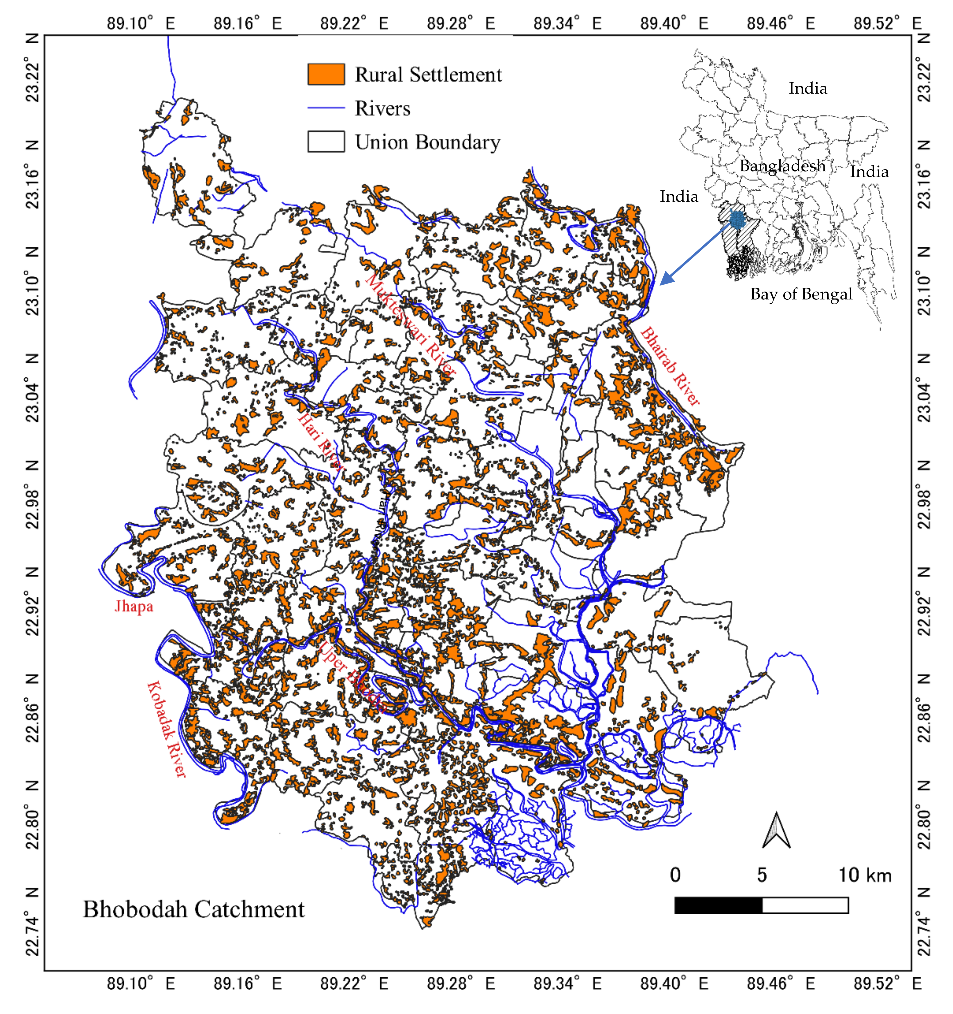
24]. The target subregions are located on the upper reaches of the FCDI project area, around 150 km from the Bay of Bengal, spreading around 1167 km2. According to population census-2011 of Bangladesh Bureau of Statistics (BBS), the population density of the target location is around 1025/km2, which is higher than the country average [25]. The explanation of choosing the upper reaches as the study area of the present study is described in the last paragraph of this section, and the detailed geographical location of the target area is presented in Figure 1.
Detection of surface water through Landsat images is not new, although several constraints exist such as (a) availability of the best quality images as expected time series points, (b) determination of the reliability and validity of the result, and (c) misclassification of land cover, particularly where multi-sectoral use of land classes exists. Broadly, three approaches were employed by the researchers to detect land classes where Landsat mission’s spectral wavelength remote sensing data were involved: 1. The single band approach engaged to describe the geographical time series distribution based on distinct threshold point, 2. Multiple band approach engaged to combine several bands, create a colorful map, and classify the image into maximum probable land use classes, and 3. Index-based or ‘ratio’ approach engaged to count spectral reflectance variations in different bands, often considered two best spectral reflectance bands to decide a context-based threshold value to finalize the index, which Du et al. described as essential to produce a better and more accurate result [26]. Exclusively detecting surface water, McFeeters had pioneered an index as the Normalized Difference Water Index (NDWI) based on green and Near Infrared (NIR) bands [27] which was later modified by Zu as the Modified Normalized Difference Water Index (MNDWI) using green and Mid-Infrared of Thematic Mapper (TM) sensors, which has almost similar wavelength with short-wave infrared (SWIR-1) band of Operation Land Imager (OLI) sensor (Table A1) [28]. Both researchers used a threshold value ‘zero’ to separate surface water from other land use classes assumed as non-water. Furthermore, Ji et al. arranged NIR, SWIR-1, and SWIR-2 bands with red band to compare NDWI threshold index characteristics and found that SWIR-1 band performed better to extract water from Enhanced Thematic Mapper Plus (ETM+) sensor data. They concluded 0.015 and -0.007 are the threshold values for NDWI and Normalized Difference Vegetation Index (NDVI), respectively, between water and non-water pixels [29]. Again, NDWI seems the best practice to identify water pixels from Landsat images where frequent seasonal water exists, such as SWB [6]. Pekel et al. used petabytes of Landsat collection-1 data for their pioneering work to present global surface water dynamics, checked the ‘seasonality and persistence’ of surface water from 1984 to 2015 using NIR, red, and SWIR-1 spectral bands [20]. On the other hand, Zhai et al. concluded that the MNDWI is a better index to extract water pixels compared to NDVI, NDWI, and Automated Water Extraction Index (AWEI), from rural and urban areas. They compared the TM and OLI sensors’ data and found that the OLI data were more efficient and stable for selecting threshold values between water and non-water pixels. To select the threshold point, first, they drew a spectral curve, then chose the values which are close to ‘endpoints’ or ‘logical value’ by sampling points values. Based on OLI data, the verified threshold values to extract waters in village areas for NDVI, NDWI, and MNDWI are 0.0, 0.0, and 0.07, respectively [30]. Similarly, Singh et al. found that MNDWI is a better index to extract water pixels that are mixed with vegetation compared to NDWI [31]. Du et al. discovered that green and mid-infrared bands of ETM+ sensor can provide better results to detect water pixels than those of green and NIR bands [26]. However, apart from Landsat mission collection-1 archival data, different remote sensing Landsat data might also produce better results: for example, Li et al. compared the conventional technique of NDWI index calculation between TM and ETM+ sensor bands data with those of Advanced Land Imager (ALI). They proved that ALI data, using the green and SWIR band, is a better index to estimate surface water compared to conventional NDWI index from Landsat collection-1 data [32]. It is important to note that the investigations which relied on the SWIR band focused on reflectance produced from the ocean, lake, and river water [26,28,32]. In contrast, a study focused on separating water pixels from mixed land classes found that the SWIR band reduces more light than the NIR band which produces more positive value, confirming that the MNDWI index has more efficiency to detect surface water. However, the study relied on Indian Remote-Sensing Satellite, P-6 data, which collects images from a coarser ground resolution than that of the Landsat observations [31]. The present study’s target location is SWB, where seasonal shallow water often exists. In such cases, the NIR band might be more efficient and effective to detect water pixels from non-water [33] and, thus, the present study assumes the NDWI index might be the more appropriate method to estimate surface water which considers green and NIR bands, instead of MNDWI which considers green and SWIR bands.
Spatiotemporal research in Bangladesh has tremendous drawbacks, such as considerations of the limited Landsat observations from different days of the year (DoY) that restricts its applicability, especially for seasonal and time series investigation. For example, ten or less than ten Landsat observations between November and April have been used to estimate eight to forty-two years of LULC and surface water change [6,18]. Furthermore, five or less than five observations between November and March have been considered for thirteen to thirty-six years of land use change detection including surface water [7,10,11,13,14,16,17] which are insufficient to produce conclusive results, especially for SWB where frequent human activity changes land classes rapidly [34]. The studies, thus, could not fulfill the need to detect and determine the extent and dynamics of surface water exclusively to observe its long-term persistence around the region. Literature on spatiotemporal change in SWB is mostly concentrated on the lower parts of the Bengal delta which are very close to the sea. Therefore, the present exploratory study aims to consider maximum available Landsat observations from 1972 to 2020 with a view to illustrating consistent, seasonal, and annual changes of surface water around the upper part of the Bengal delta. After a pilot visit in SWB, the present study carefully targets the location where it assumes that the discharging of the seasonal surface water from the basin becomes increasingly difficult for the last two decades due to rapid change of land uses around the entire coastal region and has never been considered for spatiotemporal investigation. The present study includes interviews from the local people to support the remote-sensing data and in situ information and concentrate on local mechanisms and adaptive measures if surface water becomes a spatial problem. Finally, the study includes real-time in situ training points on water and non-water grounds to produce valid information and to reduce contradictory results from Landsat collection-1 images.

2. Methodology

2.1. Study Location

The study area extends from 89.07 E to 89.45 E and from 22.73 N to 23.2 N and is located in the southwest of Bangladesh. The total population of the area is 1,196,415, according to the population census-2011 of BBS [25]. The area accommodates numerous rivers and channels which have enormous influence on the intensity of salinity and tide from the Bay of Bengal. Figure 1 shows a detailed map including physical settlement, rivers, and local administrative boundaries of the study area and its geographic location in Bangladesh. A non-government organization (NGO), ‘Uttaran’, which is working on water and sanitary issues in SWB, and a local ‘water-committee’ jointly published a report titled “History of Waterlogging in Bhobodaho Region and People’s Planning to Overcome” in Bengali in March 2019 (available at: https://uttaran.net/ (accessed on 4 January 2020)). The report detailed a chronic waterlogging scenario in a catchment in SWB spreading around three major coastal districts of Bangladesh—Jessore, Khulna, and Satkhira. The area contains forty-five unions (lowest level local administrative subdivisions) and three municipalities. The target location is in the somewhat upper reaches of the Bengal delta, around 150 km north from the Bay of Bengal, and it is commonly known as Bhabodah. The name does not represent any administrative boundary. The Bengali term is related to ‘danger from water current’ which is considered as the study area for the present study. The study area’s rivers are mostly distributaries from the Ganges (Bangladesh part). The rivers are directly and indirectly connected with the downstream part, the Bay of Bengal, which creates regular ebb and tide. During the monsoon, the tide towards the ocean is much stronger. Thereby, the southern part of the study area regularly faces more saline water intrusion than that of the north. The study area, SWB, is in the tropical region experiencing moderate winter from November to February and long wet season from June to October because of the monsoon.

2.2. Remote Sensing Data and Techniques of Analyses

The study considers remote sensing data from Earth Resources Observation and Science (EROS) of the United States Geological Survey (USGS) archival level-1 collection-1 Landsat mission’s satellite reflectance observations of 16-day temporal resolution between 1972 and 2020. Table A2 shows a total of eight Landsat missions have been accomplished during that period using four different satellite instruments. All the available previous observations have been gathered from different instruments such as (1) Multispectral Scanner System (MSS) from 1972 to 1993, (2) TM from 1983 to 2013, (3) ETM+ from 1999 to 2020, and (4) OLI from 2013 to 2020. A total of 985 observations have been counted in the entire archive focusing on the study area during the target years. Observations which have significant levels of cloud, fog, haze, and confused Tagged Image Format have been excluded for further analysis. The ETM+ sensor has gap mask data stored in a different folder inside each observational folder which have been corrected. Figure 2 shows a final total of 312 observations that have been selected for present study analysis of which the highest number has been counted as 126 from ETM+ followed by 116 from TM. Furthermore, 17 and 53 observations have been counted from MSS and OLI, respectively. Most of the valid observations were found after the 1980s.
All the short-listed observations have been converted into top of atmosphere (TOA) reflectance variations using radiometric rescaling coefficients provided in a metadata file that is delivered with level-1 collection-1 Landsat product. The TOA reflectances are used to check reflectance variations between water and non-water pixels. The following formula is employed to generate TOA reflectance:
P λ =   M p   Q c a l + A p   s i n θ S E ,
where, P λ = TOA planetary reflectance, M p = band-specific multiplicative rescaling factor, A p = band-specific additive rescaling factor, Q c a l = quantized and calibrated standard product pixel values, and θ S E   = local sun elevation angle.
The date November 16, 2020 was selected purposely to visit the study area for ground validation based on predicted Landsat-8 satellite temporal observation with a view to creating real-time training points using Global Positioning System (GPS) at different land classes. Figure A1 illustrates some of the 101 training ground points of which 41 are on water and 60 on non-water land cover. The purpose of the training grounds is to demonstrate the ranges of spectral reflectance in different wavelengths both from water and non-water pixels. The bands of OLI instruments of that field visit day of the observation were considered as ‘sample data’. Table A1 describes the sensors, bands, and the corresponding wavelengths of the OLI instrument in detail compared with the rest of the instruments. The OLI has ten different spectral bands, enveloping discrete band-specific wavelengths ranging from 0.43 µm to 12.51 µm. The study analyzes the reflectance of the first seven spectral bands with their distinct wavelengths ranging between 0.43 µm and 2.29 µm. Figure 3 displays the reflectance curve produced from different spectral wavelengths, which represents water and non-water pixels. It appears that reflectance between water and non-water training grounds in different wavelengths of Landsat-8 is clearly distinguishable.
The reflectance values produced from water and non-water training points are measured by mean (µ) and its associated standard deviation, sigma ( σ ) differences to choose the most effective wavelength ranges that have a higher capability to distinguish water pixels. Table 1 shows that band-1 and band-2 produce a considerable amount of reflectances from both training points but hardly generate any differences between water and non-water pixels. The mean reflectance in the green band is 0.094 from water and 0.093 from non-water pixels, followed by 0.071 and 0.073 from the red band. Nevertheless, the NIR band produces the highest mean reflectance of 0.25 from non-water pixels followed by 0.15 from SWIR1 and next by only 0.08 from SWIR2. In contrast, the NIR, SWIR1, and SWIR2 bands generate a significantly lower level of reflectance values from water pixels, proving that all the three bands have the capacity to differentiate water pixels from non-water ones. However, the maximum mean reflectance difference of 0.18 between water and non-water pixels is generated from the NIR band, followed by 0.13 from SWIR1 band, and next by only 0.07 from SWIR2 band. The study assumes the mean reflectance from water and non-water pixels as μ w and μ n w respectively, and similarly sigma of reflectance from water and non-water pixels as σ w and σ n w . Therefore, the study defines an index that represents the percent of separation based on normal distribution between water and non-water pixel-reflectance values r = ( μ n w σ n w ) ( μ w + σ w ) μ n w μ w × 100 (Table 1). The distribution of reflectance variations between water and non-water pixels among these three bands postulates that the NIR band has more intense efficacy in isolating water pixels from non-water pixels. The result is supported by a recent study where the NIR band is found to be a more efficient band to separate water pixels, especially from wetland where shallow water exists [33]
Based on literature and evidence from training point reflectance value analysis, the study finalizes the NDWI index to estimate surface water in the study area introduced by McFeeters which considers green and NIR bands [27]. The following formula has been employed for the index:
N D W I = ρ g r e e n   ρ N I R   ρ g r e e n + ρ N I R  
where, ρ g r e e n = reflectance from green band, ρ N I R = reflectance from the NIR band, and values greater than zero are considered as water pixels.

2.3. Threshold Selection and Reliability

The detailed distribution of training points value derived from NDWI index shows that most of the training points from water grounds are positive and all the values from non-water grounds are negative. Figure 4 shows that the mean and standard deviation of the training points of the NDWI values from water ground are 0.198 and 0.193, respectively. For non-water grounds they are −0.441 and 0.11, accordingly. Thus, it is evident that 0 would be the rational threshold value between water and non-water pixels. The study assumes that the NDWI values <0.0 produced from water training points are incorrectly identified and vice versa for those of the non-water training points.
Thus, the sample training points values of NDWI are considered for accuracy assessment through a confusion matrix process. Table 2 shows the principle of confusion matrix where 36 training points correctly classify the water pixels out of 41 and all of the 60 training points correctly classify the non-water pixels. The study employs a total of 101 training points of the NDWI values. Hence, the producer’s accuracy for water and non-water sample training pixels are measured as 87.8% and 100% respectively. Additionally, the user’s accuracy for water and non-water training pixels are 100% and 92.3%, accordingly. The overall accuracy of the confusion matrix is 92.3%. Finally, the Kappa coefficient value from the accuracy matrix is measured as 0.89. Based on the ‘classifier’ and ‘induction algorithm’, it confirms that threshold value ‘0′ has better efficacy to minimize the misclassification of non-water pixels as water pixels [35]. Table A3 and its associated formula describes the detailed calculation techniques of the accuracy assessment.

2.4. Additional Data Sources

Time series data on shrimp cultivation at different districts have been collected from the yearbook of fisheries statistics of Bangladesh [36] and yearbook of agricultural statistics of Bangladesh [37]. Field visits were completed in January and November 2020 and in March and April 2021, with a view to ensuring ground validation, observing rivers, canals, and human interventions at different locations, and conducting interviews. During field visits, a total of fifteen key informant interviews (KIIs) have been conducted from different occupational groups to support the results from remote sensing data. The primary purpose of KIIs is to understand people’s experiences of seasonality, spatiality about surface water, and its impact on land use.

3. Results

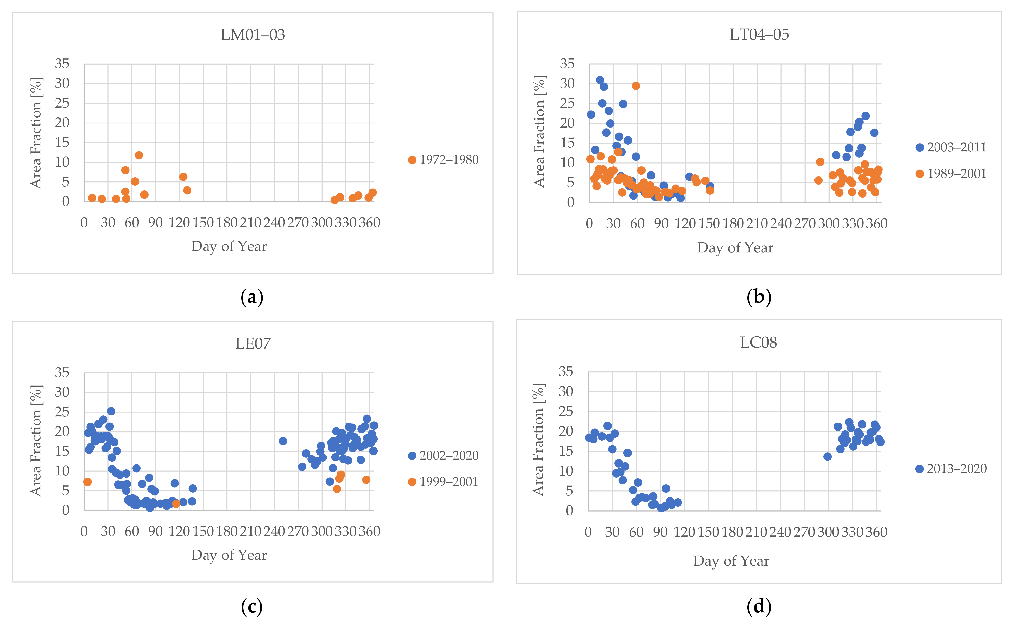
A total of 312 valid Landsat collection-1 observations from 1972 to 2020 were finally considered for analysis in the present study. A small number of observations were found between 1972 and 1980. Some observational data have been downloaded for the year 1974 and 1979, but none are considered for analysis because of the disturbed dataset in the archive. 
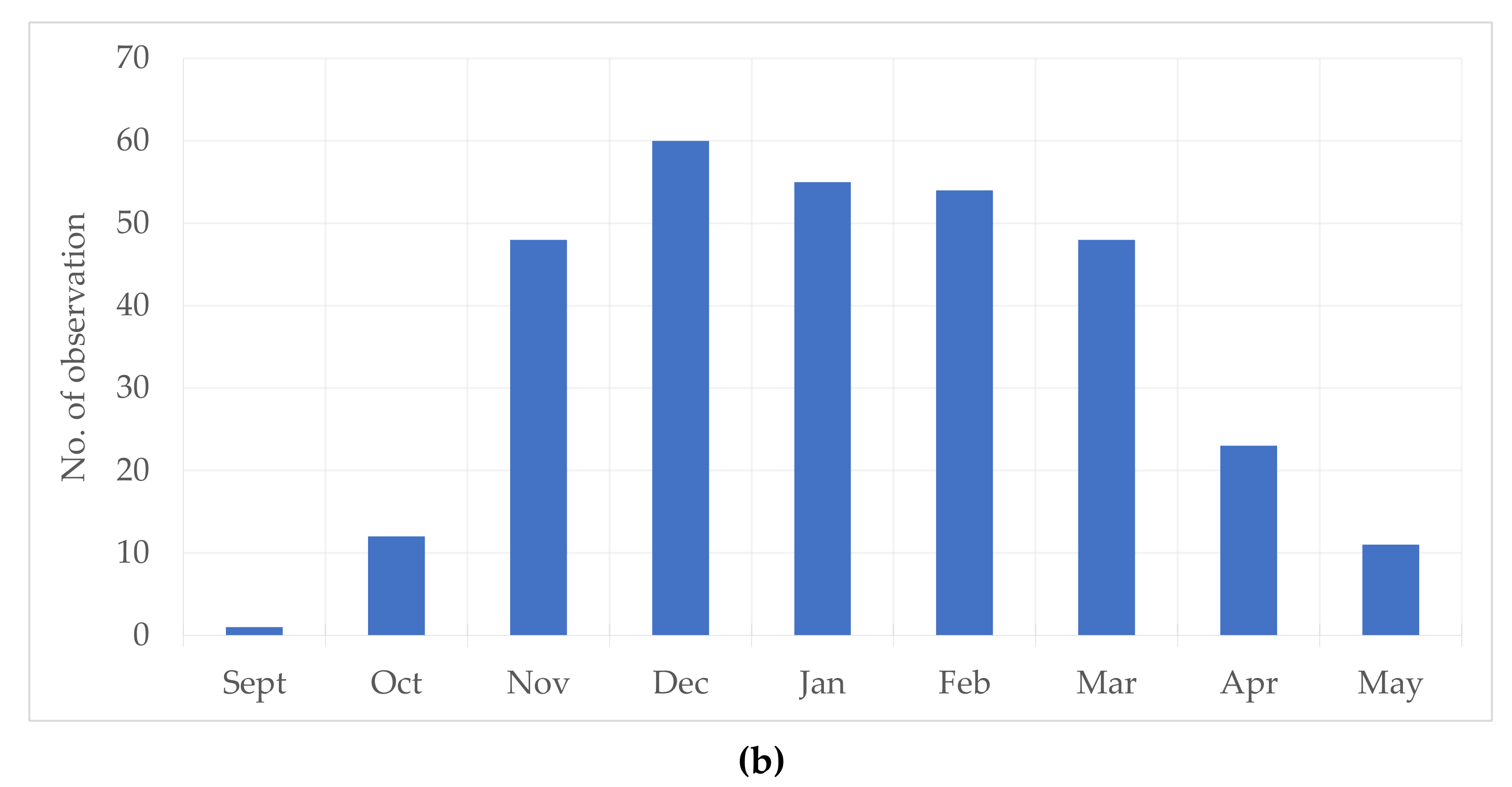
Figure 5a presents that no observation has been found between 1981 and 1986. After that, on average, six observations per year have been considered for analysis until 2003. More than twelve observations are available for each year between 2004 and 2020. On the other hand, Figure 5b shows that the highest number of observations is 60 from December, followed by 55 in January. Only one observation is available in September; thus, for monthly analysis, the month is excluded. The numbers of observations are found as 11 May and 12 October. A good number of monthly total observations are also available in February as 54 and in March as 48. No observations are considered for the final analysis for the months of June, July, and August, mainly because of the cloud coverage.
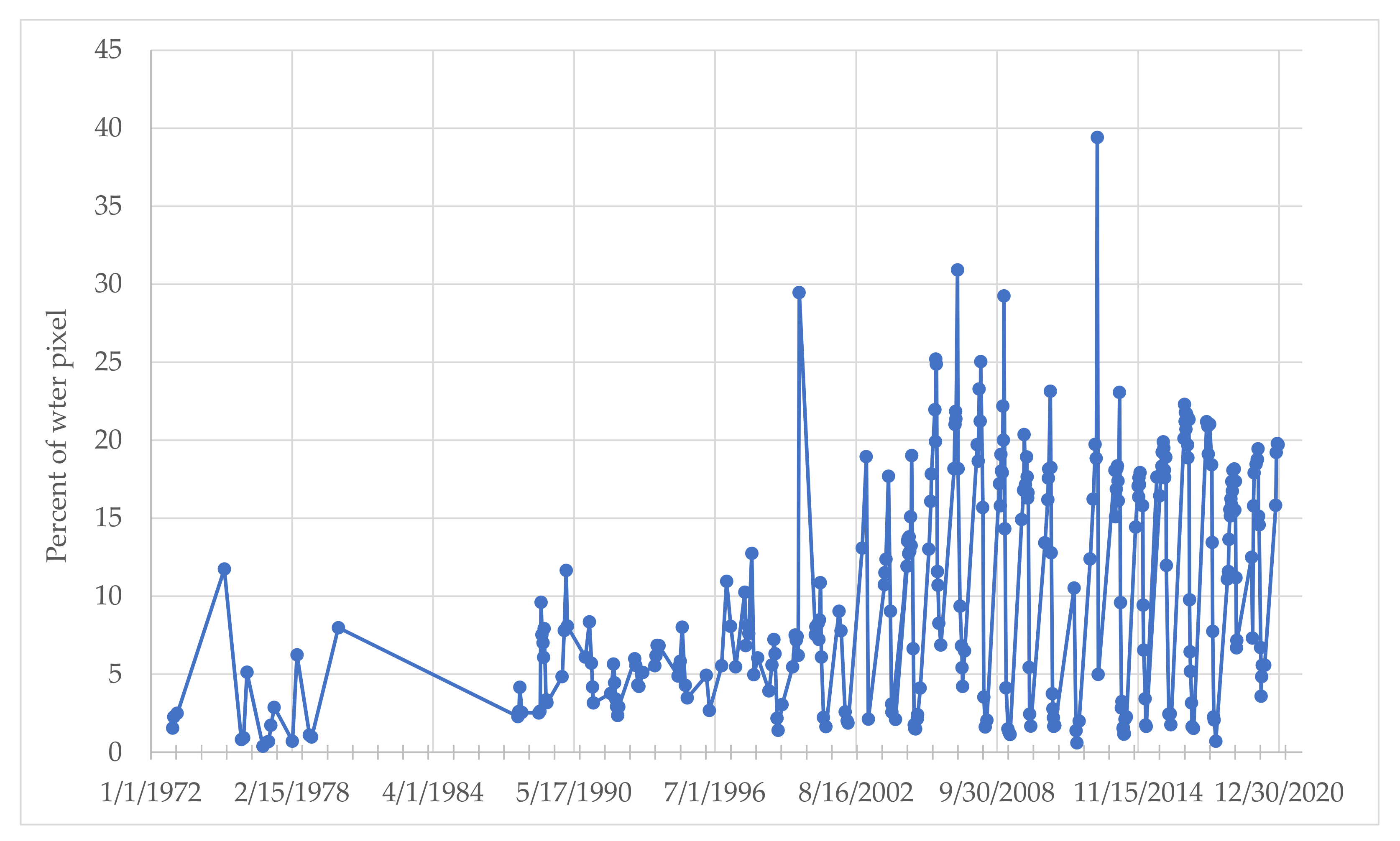
The percent of water pixels based on NDWI > 0.0 is presented to observe the general trend of percent of water bodies defined as surface water in the study area between 1972 and 2020. The years 1974, 1979, and 1981 to 1986 are not included for final data analysis based on valid Landsat observations which have already been presented in Figure 5a. The distribution of water pixels in Figure 6 distinguishes two perceivable and incompatible patterns of surface water in the study area in two different eras—(1) from 1972 to 2001 and (2) from 2002 to 2020. Though we checked for different period of separation, results do not change largely. For better understanding of temporal analysis, it is crucial to consider the analysis between these two eras, which is shown later. The NDWI > 0.0 pixels of each observation from 1972 to 2001 will be defined as the first era and, likewise, the latter part as the second era. Less than 10% area is observed as surface water in general in the first era, which expands to 20% in the second era. The highest surface water of 39.4% is observed in 2013, followed by 30.9% in 2007, and next to 29.4% in 2000. The persistence of surface water from 1972 seems uniform until 1999 and then in 2000, the first sharp increase is observed as around 29%. On an average, the study area has around 5.5% of surface water with 3.7 standard deviation in the first era which increases to 12.8% with a 7.6 standard deviation in the second era. The surface water trend could be explicitly recognized by observing the single-year distribution. The yearly presence of surface water will be presented in two different graphs representing two different eras so that it is possible to observe not only the yearly extent of surface water but also to perceive the yearly trend in two eras. Before that, a decadal change of surface water estimation is important to identify the most vital decade of surface water change in SWB. Percent of pixel trend from 1972 to 2020 presented in Figure 6 constitutes both the highest and lowest percent of surface water; in some cases, the value is too low or too high compared to the median value. The data derived from valid Landsat observations have not been distributed in a uniform frequency of the DoY. Based on the extent of the value and the diversified DoY, an interquartile range of box-plot presentations has been arranged for decadal, yearly, and seasonal analyses of the dataset using MS excel.
The study also tries to inspect the reason for some high and low values of surface water in the study area. It appears that at least 11 abrupt surface water cases which might be related to water-related natural disasters such as cyclone, riverine flood, and flash flood around SWB. Although seeking the source of surface water and its direct relationship with natural disaster is beyond the present study objective, it may be an important element to consider future remote sensing research on land class change in coastal areas of Bangladesh. Table A4 has been prepared to present surface water scenario in the study area based on the Landsat observations of the immediate before and after of the disasters. A few examples are noted—1. Surface water increases from 2.6% on 24 November to 9.6% on 10 December in 1988 are related to a category-3 cyclone on 29 November of the same year. 2. Water pixel increases from 5.5% on 25 May to 10.3% on 16 October in 1997 are related to a tropical cyclone on 26 September. 3. A category-5 cyclone on 15 November in 2007 instigated the surface water change from 6.5% on 5 May to 19.7% on 21 November. 4. Last but not least, a tropical cyclone on 9 November increased surface water from 7.3% on 6 November to 15.8% on 22 November in 1997.
From 
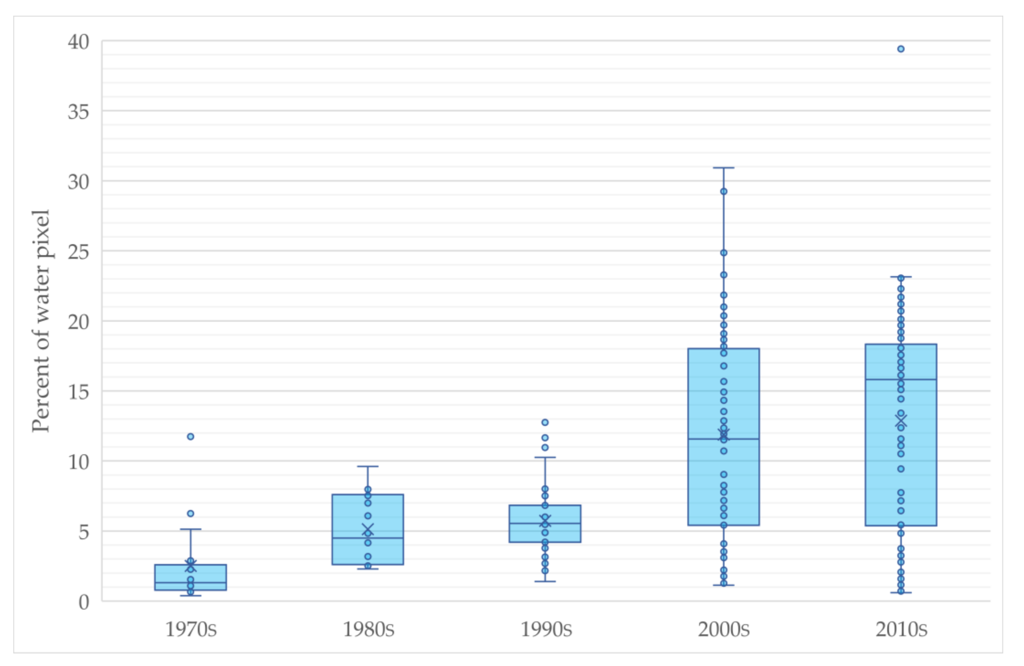
Figure 7, the presentation has been prepared through box plot analysis, where the upper whisker represents the maximum value, the lower whisker as the minimum. The upper limit of the box is based on the 75th percentile or 3rd quartile (Q3) while the lower limit is the 25th percentile or 1st quartile (Q1). The median value or 2nd quartile (Q2), and average point are shown as a line-mark and marker respectively inside the box. Dots are the actual values. The outlier dots are the values lying over 1.5 times of the interquartile range (IQR) below the Q1 or above the Q3. IQR = Q3–Q1. The study considers five decades of surface water observation in SWB between 1972 and 2020. Figure 7 reveals the decadal change, and it appears that the maximum surface water is observed as 5% and 10% in the 1970s and 1980s, respectively. The presence of surface water is only 3% in the 1970s based on Q3, which jumps to 8% in the next decade. Again, the Q3 shows that the surface water slightly decreases by 1% from the 1980s to the 1990s, but the median and maximum values indicate a slight increase of surface water between the decades. The surface water expands to the highest level in the 2000s. The maximum extent of surface water is around 10% in the 1990s, which steeply increases in the next decade. The maximum occurrence of surface water is counted as over 30% in the 2000s. It can be assumed that a two-and-a-half-fold surface water expansion occurs between the 1990s and 2000s based on Q3, while the median value of 6% is found in the 1990s that doubles in the 2000s. It is noted that a total of 51 valid observations were considered for the final analysis in the 1990s while for the latter decade the number was 93, which indicates a substantial quantity of Landsat observations were aggregated to analyze both decades. After a significant increase of surface water in the 2000s, the trend continues in the next decade as well. The IQR for the 2000s and 2010s appears almost identical. The maximum occurrence of surface water counted as over 30% in the 2000s followed by 23% in the 2010s. However, a higher median value is observed in the 2010s than that of the 2000s, which confirms that the surface water is more intense and persistent in the latter decade. However, the maximum and minimum values show that surface water decreases marginally from the 2000s to the 2010s. One extreme outlier point has been found higher than the Q3 in the 2010s. Evidently, the study area has covered much higher and distinct presence of surface water in the last two decades, the 2000s and 2010s, than that of the prior three decades which further recommends observing the extent of surface water in the two different periods which have already been defined as the first and the second era in the previous trend analysis section.
The yearly change of surface water is divided into two eras which indicates a clear and distinguishable pattern of surface water as well. Figure 8a shows that the surface water is not widely observed in the first era. In general, the median value is around 5% during the entire period. The maximum surface water is observed over 10% in four instances between 1972 and 2001. The highest surface water observed during the first era is around 12% both in 1975 and 1990, followed by 11% both in 1997 and 2001. An upper IQR is observed in the year 1990 with a minimum and maximum value as 6% and 12% respectively. Based on Q3 of the data, three waves of surface water are observed in the first era—the first wave appears between 1987 and 1990, followed by the second wave between 1992 and 1995, and the next one between 1998 and 2001. In contrast, two significant decreasing trends are also seen: the first is between 1975 and 1977 and the second is between 1990 and 1992. Two extreme outlier points are observed in 1998 and 2000 advanced the average marker out of the box plot.
Compared to the first era, Figure 8b shows significant and outspread surface water increases in the second era between 2002 and 2020. The highest maximum surface water is observed over 30% in 2007, followed by 29% in 2009. Furthermore, a maximum of 25% surface water is seen both in 2006 and 2008. In contrast, the lowest maximum surface water is observed as 5% in 2002, but an outlier value of 13% exists in that year. Around or over 20% of surface water in the Q3 is observed on at least five occasions. Based on the median value, significant increase of surface water in successive years occurred at least on two occasions—first, it increased from 5% in 2005 to over 20% in 2006, and the second, 6% in 2012, increased to around 18% in 2013. Around 13% of average surface water is observed in four consecutive years from 2007, then it decreases until 2012 to around 8%. A sharp increasing trend is observed from 2014 to 2016, then it slightly decreases next year. However, from 2017, the surface water appeared to increase until 2020. Two outlier values higher and lower than the Q3 and Q1 are observed in 2013, and the median value is 18%.
The percent of pixel based on NDWI > 0.0 in the study area is arranged in monthly order from October to May contemplating all the available observed data between 1972 and 2020. Figure 9 demonstrates that the months—June, July, August, and September—are excluded from the analysis either because of the absence of valid observations or the presence of very few observations. The highest maximum surface water is observed in January at over 30% followed by 25% in February. The maximum value for both December and November is observed as around 23%. In contrast, the maximum value for March, April, and May is found around 5%. The Q3 shows that the surface water in the study area is 14% in October, which sharply increases to 18% in November, increases further 1% in December, and remains the same in January. However, after January the drastic change began, as surface water went down to 13% in February and again to only 4% in March and 3% in April. The median value of surface water in May is only 5%. The IQR of the month from November to February shows the most consistent and extensive surface water in the study area. The IQR of November, December, and January is almost identical, but the highest median value in January proves that the month has the higher consistency of surface water. A considerable level of surface water in October is found compared with the two sets of months shown by the two box-markers in Figure 9. This eight-month observation of surface water in the study area provokes further analysis between the two groups of months. Group-A, when a significant presence of surface water appears, including November, December, January, and February; and group-B, when a minimum percent of surface water exists, including March and April, and May in between the two eras. The significant decrease of surface water observed between January and February, and February and March, is also notable.
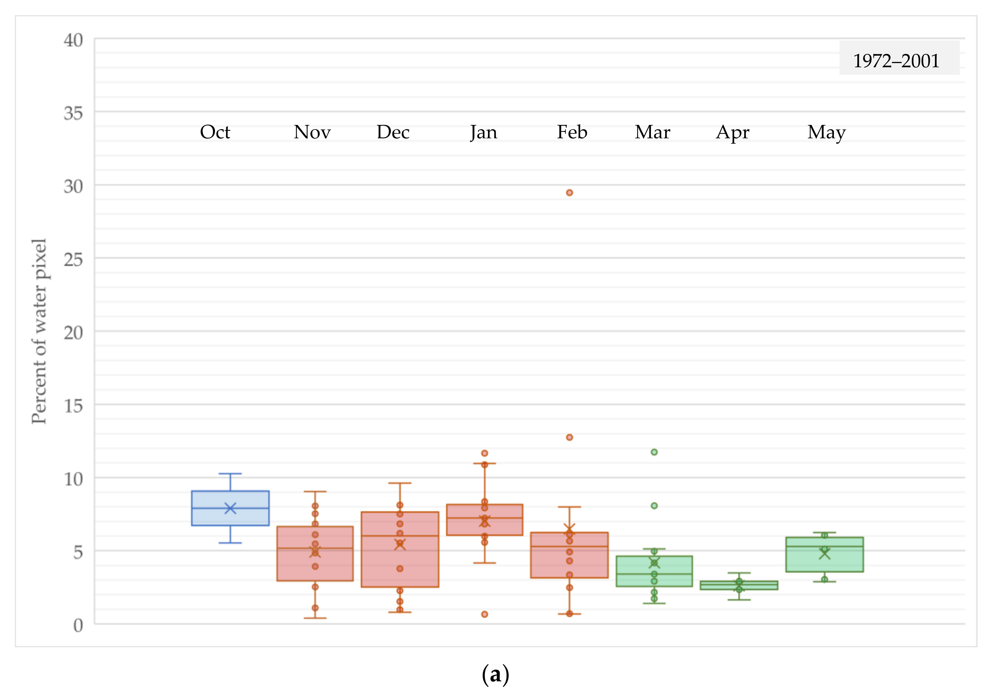
Figure 10 presents the monthly trend of surface water between the two eras—from 1972 to 2001 and from 2002 to 2020; group-A and group-B months are colored differently while the month October remains the same color. Figure 10a reveals that the maximum monthly surface water in group-A months in the first era is around 10% while in group-B months it is around 5%. The box plot of group-B months indicates a similar intensity and trend of surface water as the monthly analysis presented in Figure 9. In addition, for the group-A months, the Q3 of surface water in November is found around 7% which increases by 1% in the consecutive two months as 8% in January. A slight decrease trend is also observed from January to April. Two outlier points are available among each of the observations from the month of January, February, and March. On the other hand, compared to the first era, Figure 10b shows a completely different consistency and extent of surface water from 2002 to 2020. The maximum surface water appears in February as around 25%, followed by around 23% both in December and January. The widest IQR appears in February where Q3 and Q1 are 15% and 6% respectively. The Q3 of the value suggests an increasing trend of surface water from November to January. However, the change of surface water is much wider and clearer between January and February, and February and March. Such successive monthly change of surface water never appears in the first era. The extent of surface water in the study area for the months of November, December, January, and February seems to expand nearly two-and-a-half fold in the second era as maximum value is found to be more than 23% in each case. The extent is so clear that the minimum values of Group-A months in the second era are always higher than that of the maximum value from the first era. In contrast, the trend and extent of surface water for the months of March, April, and May remains almost the same in both eras as the maximum value appears around 5%, while water fraction seems to decline from March to April in the second era. However, the surface water is seen to increase slightly in October in the second era. Thus, the reasons for the significant increase of surface water in the study area for group-A months and drastic change from January to April in the second era need to be clarified in the discussion section.

4. Discussion

4.1. Recent Situation of Surface Water

The present study area is located in three different districts of Bangladesh—Jessore, Khulna, and Satkhira. Total area of the target location is 11,674 hectares (ha.) of which 81% is in Jessore (northern part of the study area), followed by 15% and 4% located in Khulna and Satkhira districts (southern part of the study area), respectively. To explore the recent persistence of surface water, the study compares the persistence of surface water around the study area at different locations for the year 2020. A bar diagram in Figure A2 has been arranged in different colors, where blue color shows the percent of surface water in the study area, red color for Khulna portion, gray color for Jessore portion, and yellow color for Satkhira portion. A total of fifteen valid Landsat observations have been counted in different DoY of 2020 based on Landsat 7 and 8. Three valid observations have been found from each month of January, February, and March and two from each month of November and December. Only one observation has been found between April and May. The study area experienced around 18% of surface water on 1 January, which almost remained the same until 2 February, then it decreased to 15% on 10 February, which continued throughout the month. A drastic decline is observed after the end of February, to 6.7% on 13 March. It further declined to 3.5% in the same month, which ranks the lowest level of surface water in 2020. The trend of surface water in 2020 at Khulna and Jessore regions follows that of the study area while the Satkhira region remains different. The highest percent of surface water is observed at the Khulna area, the southeastern part of the study area, in all the observations in 2020 (Figure A2). Based on the spatial distribution of the surface water in the study area, four patterns are observed in 2020, illustrated by four boxes in Figure A2: (1) first week of November, (2) from the second week of November to the first week of February, (3) from the second week of February to the end of the month, and (4) from the first week of March to the third week of May, which is presented in the study area’s surface water binary map in Figure 11. It appears that the study area’s rural settlements roughly correspond with water fractions (Figure 1 vs. Figure 11a) and river shape areas at the Khulna portion or southeastern part of the study area also seem waterless (Figure 1 vs. Figure 11b). However, intense surface water spatiality mostly concentrates at the southeastern part of the study area in 2020. The northwestern part of the study area looks dry in 2020 except for December and January (Figure 11a,c,d vs. Figure 11b). Surface water hardly exists between March and May at Satkhira portion—southern part (Figure 11d). A wider seasonal change of surface water has developed in the Jessore portion—the northeastern part of the study area (Figure 11b vs. Figure 11d). The highest persistence of surface water is exposed at the Khulna portion between November and January—the southeastern part of the study area (Figure 11b).

4.2. Reasons for Widespread and Prolonged Surface Water in Southwest of Bangladesh after 2001

The first cause of widespread and prolonged surface water at SWB in Bangladesh in the second era is identified as water management projects and human interventions. After FCDI projects during the 1970s and 1980s, the government implemented a new project at SWB in the 1990s—the Khulna-Jessore Drainage Rehabilitation Project (KJDRP)—with a view to increasing the free flow of local water through rivers and canals to the major rivers with the help of structural solutions such as constructions of huge water regulators. The KJDRP had received tremendous community protests because after just a decade of implementation, surface water from the monsoon season (June–October) gradually increased to remain static until the dry season (November–February) in the upper reaches of the project, which is the target location of the present study. During the period, the channels and rivers, especially Bhadra, Hari, Mukteshwari, and Shalgatia, which are vital for drainage of seasonal water from the study area, have received rapid silt deposition. The river Hamkura, which is inside the present study area, has been found to have perished. Consequently, local people formed a ‘water-committee’, demanded depolderization, and cut several polder embankments hoping for natural flow from the tidal river. In the late 1990s people also demanded the implementation of regional Tidal River Management (TRM) to address static water problems. The concept of TRM is to allow tidal flow in the basin, which increases tidal volume, stores floodwater, and traps sediment during long storage periods of sedimentation. The target of TRM was to raise the basin-bed through siltation to pass the trapped water through local rivers. Finally, in 2000, the Bangladesh Water Development Board (BWDB) agreed to implement TRM as a method of water and basin management. Though the concept of TRM comes from local people, it demands nearly a perfect and systematic implementation approach such as area selection and calculation of the duration and amount of sediment required to be successful. Again, local people claimed that authorities ignored their idea of using natural flow from the river tides. Instead, they used mostly water regulators to increase the sedimentation which ultimately changed the local people’s land into a permanent wetland [4]. Though tidal basin management is more ecofriendly and more cost-effective [38], it has been not only increasing the river and canal’s bed but also intensifying surface water in the vast region of upstream catchment such as water bodies in Jessore, Khulna, and Satkhira districts due to unplanned implementation approach, institutional limitations, mismanagement, and social conflicts during the last two decades [39,40,41].
Several field visits of the present study also revealed that most of the rivers around the study area are located in the southern part that are vital for discharging the study area’s seasonal water to the major rivers. Numerous canals and channels connect the local rivers with beels. The observation and KII confirmed that the canals and local rivers have hardly any water tide now, and one river has even perished. Figure 12a shows the upstream of the Shalgatia river which has been turned into aquaculture by the local people through building temporary mud-embankments affecting free flow during monsoon and reducing the tide in the downstream of the river. In Figure 12b, human intervention appears on the riverbank, downstream of the Shalgatia river. Figure 12c shows that there is hardly any water tide in the Hari river which is important to pass the water flow from the southeastern part towards the major rivers. Figure 12d presents the static surface water at an elementary school at Shundali union in the northeastern part of the study area. A farmer from Rudhagara union described the decadal changes of canals and rivers as follows.
“Lack of water-tide and seasonal sedimentation have been raising the bed of canals and rivers around my areas. For example, during my childhood (around 30 years ago), I saw my local river named Hamkura has ebb and tide regularly, and now you cannot find any river but some marks. Local people are using the rivers to cultivate rice fields and to farm fish. Similarly, the canals and channels which connect beel and river have no water flow at all, even during the monsoon. Finally, it affects the local rivers (Hari river and Sholgatia river) that relate to other big rivers downstream. I can remember just 30 years ago people couldn’t cross the river by swimming, and now it is too narrow and too shallow to walk through the river easily. That is making static water in our beels”.
In addition to the hydrological management, the second factor for widespread surface water in SWB is the rapid land use change around the region. The flood controlling policy and water management projects had encouraged people for earthworks [5] around their localities since the 1970s. Simultaneously, people utilized the static water for income-earning activities, a resilient practice–aquaculture, which Pekel et al. clearly identified as ‘new permanent’ water in their remarkable research. They found an enormous increasing trend of surface water between 1984 and 2015 assuming a change from seasonal agricultural wetland to static water–aquaculture [20]. The spatiotemporal data of the present research and the secondary data on shrimp farms in SWB also confirm a rapid change of land use, such as shrimp cultivation which not only fulfills the local nutritional demand but also meets the increasing demand from the global shrimp market. Figure 13 shows a sharp expansion of shrimp cultivation land just after 2002 in Khulna, and Satkhira districts. Such expansion in the Jessore district is seen after 2006. In the Jessore district around 895 ha. of land was under shrimp cultivation in the fiscal year (FY) 1995–1996 which rapidly increased to 6544 ha. in FY 2004–2005 and 18,776 ha. in FY 2018–2019. The highest area covered for shrimp cultivation is found around 80,009 hectares—a total of 35.2% of the total district land of Khulna in FY 2016–2017. Similarly, around 36% and 9% of the district land of Satkhira and Jessore respectively are seen under shrimp farms. A local farmer from Khulna, the southeastern part of the study area, described the land use change experiences as follows:
“I remember the year when villagers converted their one-cropped-land into fish farming. It was after 1996. Because sudden flooding came to our beel in 1995 due to the rising water level of our local rivers and an extensive inundation around downstream areas. The flood damaged the entire village’s rice production and water was stuck for a few years, and simultaneously we started to enclose our farmland to construct fish farms not only to produce fish but also to protect rice fields from flooding. The change gradually intensified within a decade”.
The time period of the expansion of shrimp farms at the particular locations of the study area is also supported by the spatiotemporal results of the present study, demonstrated for example by Figure 11a–d, which show that the surface water is located in the southernmost location of the Khulna portion around the year 2020. Shrimp farm data from Khulna in Figure 13 also suggest an early expansion of aquaculture in the district.
The interview also reveals that the surface water and the water-tide from the local river are very important for cultivating shrimp in SWB, which starts preparation in early June and ends harvesting in early November. The preparation often starts inside the shrimp farm in May by drying up the entire land, which is very similar to the result of the monthly trend of surface water presented in Figure 9. After November, again, they need irrigation water to produce Boro rice in the same land. The Boro rice plantation starts from mid-December to mid-January and converts the entire land—shrimp land and farmland—virtually into a wetland from November to January. The binary image of scattered water fractions at the northwestern part of the study area has already been converted into irrigation water during January, presented in Figure 11b. Then, the grown rice plant started to cover-up the dried shrimp farm between March and April. The harvesting time of the Boro rice is the end of April. Such mix-cropping, expanded mostly after 2000, is exposed as vital for the local economic prosperity. This seasonal use of surface water has already appeared through remote sensing analysis presented in Figure 10b and surface water map on 6th April 2020 in Figure 11d. However, the farmers need to drain the surface water to the river after January through the narrow and zigzag canals and channels, which is tremendously difficult, especially after 2000. The interview regarding seasonal land-use confirms the extent of surface water in group-A months and the rapid decreasing change between January and March, which has already been presented in Figure 9. However, the canals and channels are not regularly maintained, and if maintenance is needed, it often relies on voluntary labor provided by the local people without any master plan involved. The flow of water through the canals is also obstructed due to its line-up through the highly fragmented pieces of shrimp-farm embankments. The situation is described well by a farmer from Jessore, the northeastern part of the study area:
“We obviously need water for both shrimp and rice cultivation, especially for the Boro rice production. The great problem we are facing now-a-days to pass the local water to the river after late December. So, we gathered as a team to work to clear the canals and channels that connect the nearest river before the Boro rice season which is not entirely enough for a free flow of water. The mix cropping really helped me a lot personally. Compared to twenty years ago, before the conversion of my land into mix cropping, my income increases almost double now”.
The expansion of the shrimp area and rapid pace of Boro rice cultivation especially after the year 2000 [42,43] further validate the extensive surface water and its monthly change in group-A months in SWB after 2001.

4.3. Validation of Spatiotemporal Remote Sensing Time-Series Data

The present study has already validated the reasons for using green and NIR bands, NDWI index, and threshold point between water and non-water pixels, based on the ground truth training points value produced from OLI sensor (Table 1 and Figure 4). For constructing time-series remote sensing data between 1972 and 2020, the investigation relies on the same threshold point applicable for MSS, TM, and ETM+ sensors as well. However, these sensors have different wavelength ranges than those considered for the NDWI index (Table A1). Thus, a comparison has been arranged between percent of NDWI > 0.0 pixels of the OLI sensor and that of the other sensors (Figure 14d vs. Figure 14a–c). The data have been arranged to visualize by (1) Landsat product identifier name assigned for each sensor and its number such as MSS as LM, TM as LT, ETM+ as LE, and OLI as LC; (2) separating the two eras, 1972–2001 in brown color and 2002–2020 in blue color; and (3) distribution ranges from 1 to 365 (or 366) based on DoY. Figure 14 illustrates that very few of the data are observed between 120–300 DoY, mainly because of the compromised Landsat data as a result of the cloud coverage. The data from LT are distributed almost equally between the eras (Figure 14b). The value acquired from the LT and LE spreading from 1989 to 2020 follows the distribution of LC, and the decreasing trend, from 32 to 59 DoY, representing the month February, is almost identical in TM, ETM+, and OLI (Figure 14d vs. Figure 14b,c). The trend confirms that the result produced from OLI sensor for surface water estimation based on NDWI index is also equally applicable for TM and ETM+ sensors data. Though the number of valid observations from LM are limited, it also somehow follows LT (Figure 14b vs. Figure 14a). Thus, the trend distribution of percent of NDWI > 0.0 indicates reliable and valid data produced from OLI that are applicable for all the other previous sensors.

5. Conclusions

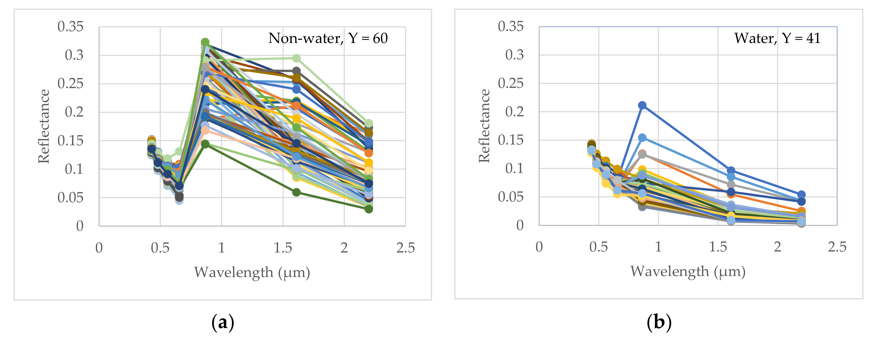
The present remote sensing study explores the trend, extent, and seasonality of surface water at the southwestern part of Bangladesh based on maximum useable Landsat level-1 reflectance observational data. The main limitation of reflectance data is cloud coverage; thus, the study excludes the months between June and August and cannot focus on the years between 1979 and 1986 due to the disturbed dataset. The study discusses numerous water management projects and frequent natural disasters around SWB but does not try to provide concrete evidence that these events might be the source of surface water on the upper reaches of the Bengal delta. However, the interviews reveal the decadal change of human interventions; seasonal water management by the locals, especially using the surface water for their better livelihood; and at least 11 natural disasters that might trigger surface water between 1972 and 2020. Further studies on the impact of natural disasters such as storms, tropical cyclones, and floods and the consequences of water management projects on surface water considering the entire delta may be needed. The reflectance analysis of the investigation, based on the real-time ground truth data, suggests that the NIR band has the highest separation efficacy between water and non-water pixels compared to SWIR1 and SWIR2. The threshold value ‘0′ of NDWI based on OLI sensor image to detect surface water produced an overall accuracy of 92.3% where the Kappa coefficient value is 0.89. The study also confirms the threshold value as reliable and applicable to other previous sensors of the Landsat level-1 archival data as well (Figure 14). Thus, the study ensures and suggests using NIR band and NDWI index as a reliable method to estimate surface water, especially from other parts of Bangladesh where frequent and seasonal land class change and shallow surface water exist. Similar analysis may be applicable to the region where complex aquaculture and paddy field cultivation are actively conducted. The method based on NDWI may be applicable at least from the TM sensors. However, the study recommends checking the threshold value against the ground truth. Based on people’s past experiences of land use and historic secondary data, the study confirms that human interventions transformed the spatiality of surface water in SWB, mostly between November and February, particularly after 2001. On average, the SWB has faced around 5.5% of surface water between 1972 and 2001, which increased to 12.8% between 2002 and 2020. The median surface water doubled from the 1990s to the 2000s and nearly tripled in the 2010s (Figure 7). The highest median value of surface water was observed around 18% in January and the lowest, just over 2%, was observed in April between 1972 and 2020 (Figure 9). Monthly comparison between the two periods—from 1972 to 2001 and from 2002 to 2020—suggests that average surface water expanded from 5% to 17% in November, from 6% to 18% in December, 7% to 19% in January, and from 6% to 11% in February. In contrast, the average surface water slightly decreased in March, April, and May. Hence, based on the trend, extent, and seasonality of surface water in SWB, the study suggests using December and or January month’s Landsat observations, especially for studies which involve identifying LULC where waterbody or surface water is either exclusive or one of the land classes in southwestern Bangladesh. It appears that the aquaculture, especially the shrimp farm, is the primary source of surface water and one of the key livelihood options for the people in SWB. Thus, to estimate shrimp farm might be an important option in future remote sensing research which may provide almost real-time monitoring opportunity for the policy makers. Surface water is not only important for the flora and fauna but also for local ecology. The study finds a tremendous seasonal change in SWB after 2001 and assumes it also affected the local ecology such as humidity and surface temperature. Such changes of surface water obviously influence people to fabricate their livelihoods, which may transform the community and even society. The future research regarding ecological effects from surface water, adaptation research, and social impact might be crucial for the academicians and planners in Bangladesh.
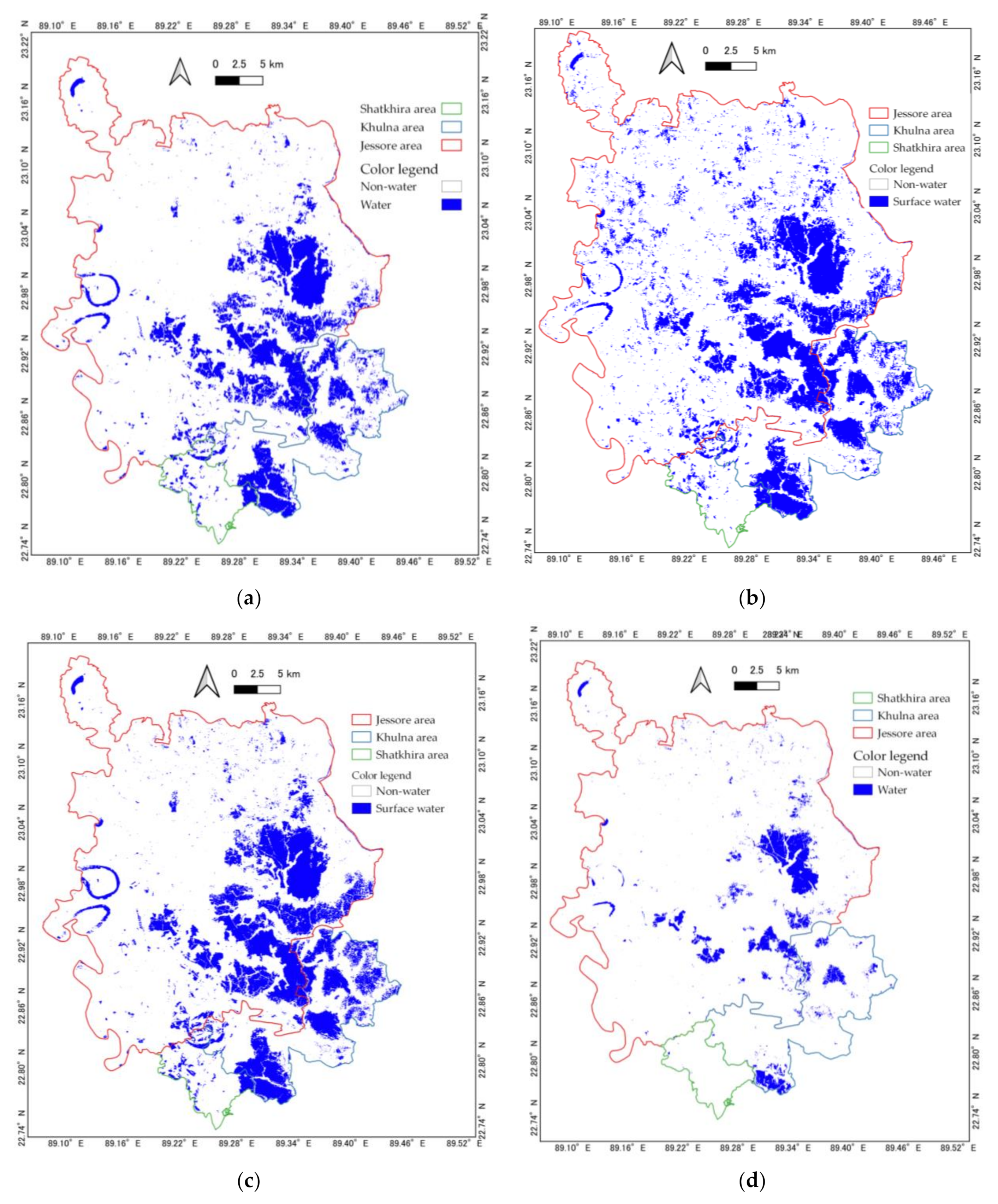
Based on the water pixel analysis and interviews, in short, the reason for widespread surface water between October and mid-November after 2001 (Figure 10b) is the increasing trend of aquaculture, especially shrimp cultivation (Figure 13). The source of water for the shrimp farm is local rivers, which are easy to collect from the elevated water-level during the monsoon. In study the areas the local rivers are closely connected to the Bay of Bengal, and frequently carry salty water that is suitable for shrimp farm production but not for paddy cultivation. The highest expansion of surface water observed between mid-November and early February (
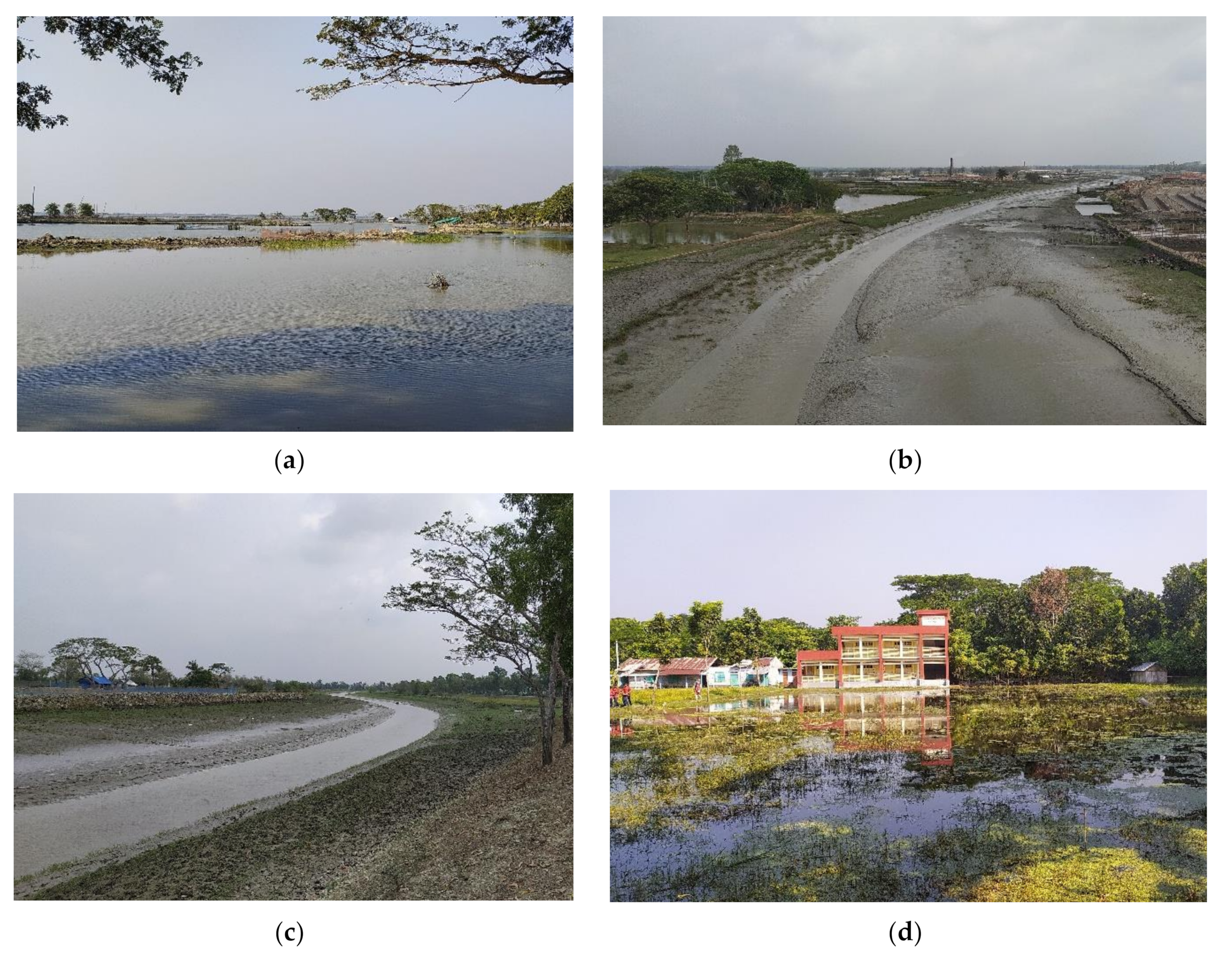
Figure 10b) was mainly because of water management by local people. The entire beel, including fish-farms, is divided by large-scale temporary embankments to discharge the surface water and reduce the water level so that the farmers are able to plant Boro rice. The interview also confirms that such water management was never needed before 2002 because the monsoon water from beel was automatically discharged through downstream rivers. This discharged water, interrupted by local canals, rivers, and downstream earthworks (Figure 12a,b), expands in unexpected areas such as human settlements, educational institutions (Figure 12d), and even local roads, particularly between mid-November and early February in each year from 2002 (Figure 11b,c). During the entire Boro rice season inside the embankments, primarily, the farmers use groundwater to avoid the salty water from the shrimp farm which remains as a water reservoir. After February, gradually, the rice plant covers the study area’s cultivable land and the logged water in the local settlements dries due to evaporation and penetration into the ground because of the summer season (Figure 11d). This study has already addressed the expansion trend of rice cultivation, which follows that of shrimp cultivation, especially after 2001 [42,43].

Author Contributions

Conceptualization, writing—original draft preparation, and validation, N.H.; formal analysis, investigation and data curation, N.H. and T.T.; writing—review and editing, A.N. and T.T.; methodology, software, and visualization, N.H., T.T. and A.N.; supervision, Y.S. All authors have read and agreed to the published version of the manuscript.

Funding

This research was supported by the “Fellowship grants of 2018–2019 Fiscal Year (3rd Round) for Higher Education and Research in ICT”, ICT Division, Ministry of Posts, Telecommunication and Information Technology, Government of the People’s Republic of Bangladesh; The 8th Precipitation Measurement Mission (PMM) and the 2nd Research Announcement on the Earth Observation (EORA) by the Japan Aerospace Exploration Agency (JAXA), and; the Grants-in-aid for scientific research (20H02252 and 20H01523), by JSPS.

Data Availability Statement

Temporal remote sensing data were collected from Earth Resources Observation and Science (EROS) of the United States Geological Survey (USGS) archive level-1 collection-1 Landsat mission’s satellite. Available online: https://earthexplorer.usgs.gov/ (accessed on 4 April 2020). Historical natural disasters data were collected from Emergency Events Database (EM-DAT), Centre for Research on the Epidemiology of Disasters (CRED), Brussels, Belgium. Available online: www.emdat.be (accessed on 24 February 2021). Population and aquaculture data were collected from digitization of Bangladesh Bureau of Statistics (BBS) reports, Dhaka, Bangladesh. Available online: http://www.bbs.gov.bd/ (accessed on 19 May 2021).

Acknowledgments

This work was conducted as a joint research program of Center for Environmental Remote Sensing (CEReS), Chiba University (2020 and 2021). We would like to thank Badsha Molla and Jinarul Islam from Bangladesh for their support and assistance during data collection and geo-coordination for this research.

Conflicts of Interest

The authors declare no conflict of interest.

Appendix A

Table A1. Comparison of wavelength from different bands of OLI with previous Landsat instruments.
Landsat Sensor of OLIWavelength Range of OLI Wavelength Range of ETM+Wavelength Range of TMWavelength Range of MSS
Band 1—Coastal aerosol0.43–0.45
Ban—Blue0.45–0.51B1 (0.45–0.52)B1 (0.45–0.52)
Ban—Green0.53–0.59B2 (0.52–0.60)B2 (0.52–0.60)B1 (0.5–0.6)
Ban—Red0.64–0.67B3 (0.63–0.69)B3 (0.63–0.69)B2 (0.6–0.7)
Ban—NIR0.85–0.88B4 (0.77–0.90)B4 (0.76–0.90)B3 (0.7–0.8)
Ban—SWIR 11.57–1.65B5 (1.55–1.75)B5 (1.55–1.75)
Ban—SWIR 22.11–2.29B7 (2.09–2.35)B7 (2.08–2.35)
Ban—Pan-Chromatic0.50–0.68
Ban—Cirrus1.36–1.38
Band—TIRS-110.60–11.19
Band—TIRS-211.50–12.51
Table A2. Landsat mission details and total observation considered for analysis.
InstrumentLandsat MissionRow PathAcquisition PeriodGround Resolution (m)Total Observation AvailableConsidered for Analysis
MSS1–31480441972–1983605717
3–41380441989–19936030
TM4–51380441983–201330374116
ETM+71380441999–202030376126
OLI81380442013–20203017553
Total 985312
Source: U.S. Geological Survey, Landsat mission.
Figure A1. Examples of training points at different land classes in the study area. Landsat image of 16 November 2020.
Sustainability 13 09798 g0a1
Table A3. Accuracy assessment based on training points value of NDWI.
Reference Value
WaterNon-WaterTotal
Classified valueWater36036
Non-water56065
Total4160101
Assume that OA = overall accuracy, AC = agreement by chances or expected agreement, PCT = producer’s column total, ACT = user’s column total, TS = total sample.
OA = No .   of   correctly   classifed   water   pixel + No .   of   correctly   classifed   non water   pixel 101 = 36 + 60 101 = 0.95 = 95 % AC = PCT 1 ÷ TS × ACT 1 ÷ TS + PCT 2 ÷ TS × ACT 2 ÷ TS = 41 ÷ 101 × 36 ÷ 101 + 60 ÷ 101 × 65 ÷ 101 = 0.405 × 0.356 + 0.594 × 0.643 = 0.14418 + 0.38194 = 0.52612 K a p p a   c o e f f i c i e n t = OA AC ÷ 1 AC = 0.95 0.526 ÷ 1 0.526 = 0.424 ÷ 0.474 = 0.8945 = 89.5 %
Table A4. List of natural disasters in SWB from 1970 to 2020.
No.DoY and Type of DisasterAffected DistrictsTotal DeathDoY of LS ObservationSurface Water (%)
119-11-1988
Category 3 cyclone
Jessore, Khulna, Satkhira100024-11-19882.6
10-12-19889.6
226-09-1997
Category 4 cyclone
Khulna18825-05-19975.5
16-10-199710.3
3**-07-2002
Flash flood
Jessore, Satkhira 1013-04-20021.9
23-11-200213
424-08-2006–20-09-2006
Riverine flood
Jessore, Khulna, Satkhira*24-04-20066.9
18-11-200618.2
515-11-2007
Category 5 cyclone
Khulna, Satkhira423405-05-20076.5
21-11-200719.7
625-05-2009; 29-07-2009
Category 1 cyclone; Riverine flood
Khulna, Satkhira, Jessore;
Khulna
190; 1024-04-20091.1
25-10-200914.9
701-10-2010–12-10-2010
Riverine flood
Khulna, Satkhira1518-03-20101.7
28-10-201013.4
825-07-2015–27-07-2015
Riverine flood
Khulna1124-03-20151.6
26-10-201516.4
910-08-2017–31-08-2017
Flood
Jessore14414-04-20171.5
08-11-201721.2
1004-05-2019
Category 5 cyclone
Khulna, Satkhira3903-03-20197.2
21-10-201912.5
1109-11-2019
Category 3 cyclone
Satkhira, Khulna4006-11-20197.3
22-11-201915.8
* Data is not available. Source: The Centre for Research on the Epidemiology of Disasters (CRED) [44].
Figure A2. Percent of surface water at different locations in the study area on different dates in 2020. Four different patterns are observed, illustrated by four boxes.
Sustainability 13 09798 g0a2

References

  1. Valipour, M.; Bateni, S.M.; Dalezios, N.R.; Almazroui, A.; Heggy, E.; Şen, Z.; Angelakis, A.N. Hydrometeorology: Review of Past, Present and Future Observation Methods. In Hydrology; Hromadka, T.T., Rao, P., II, Eds.; IntechOpen: London, UK, 2021; pp. 1–26. [Google Scholar]
  2. Asian Development Bank (ADB). Khulna-Jessore Drainage Rehabilitation Project: Performance Evaluation Report, Mandaluyong, Philippines. November 2007, pp. 1–49. Available online: https://www.adb.org/sites/default/files/evaluation-document/35104/files/21087-ban-pper.pdf (accessed on 14 June 2020).
  3. Rahman, A. Beel Dakatia: The Environmental Consequences of a Development Disaster; University Press Limited (UPL): Dhaka, Bangladesh, 1995; ISBN 9840512587. [Google Scholar]
  4. Nowreen, S.; Jalal, M.R.; Khan, M.S.A. Historical analysis of rationalizing South West coastal polders of Bangladesh. Water Policy 2014, 16, 264–279. [Google Scholar] [CrossRef]
  5. Adnan, M.S.G.; Haque, A.; Hall, J.W. Have coastal embankments reduced flooding in Bangladesh? Sci. Total Environ. 2019, 682, 405–416. [Google Scholar] [CrossRef]
  6. Ahmed, K.R.; Akter, S. Analysis of landcover change in southwest Bengal delta due to floods by NDVI, NDWI and K-means cluster with Landsat multispectral surface reflectance satellite data. Remote Sens. Appl. Soc. Environ. 2017, 8, 168–181. [Google Scholar] [CrossRef]
  7. Karim, M.F.; Zhang, X.; Li, R. Dynamics of Shrimp Farming in the Southwestern Coastal Districts of Bangladesh Using a Shrimp Yield Dataset (SYD) and Landsat Satellite Archives. Sustainability 2019, 11, 4635. [Google Scholar] [CrossRef] [Green Version]
  8. Islam, S.M.D.; Bhuiyan, M.A.H. Impact scenarios of shrimp farming in coastal region of Bangladesh: An approach of an ecological model for sustainable management. Aquac. Int. 2016, 24, 1163–1190. [Google Scholar] [CrossRef]
  9. Hossain, M.S.; Uddin, M.J.; Fakhruddin, A.N.M. Impacts of shrimp farming on the coastal environment of Bangladesh and approach for management. Rev. Environ. Sci. Biotechnol. 2013, 12, 313–332. [Google Scholar] [CrossRef]
  10. Akber, M.A.; Khan, M.W.R.K.; Islam, M.A.; Rahman, M.M.; Rahman, M.R. Impact of land use change on ecosystem services of southwest coastal Bangladesh. J. Land Use Sci. 2018, 13, 238–250. [Google Scholar] [CrossRef]
  11. Rahman, M.M.; Begum, S. Land Cover Change Analysis around the Sundarbans Mangrove Forest of Bangladesh Using Remote Sensing and GIS Application. J. Sci. Found. 2011, 9, 95–107. [Google Scholar] [CrossRef] [Green Version]
  12. Johnson, F.A.; Hutton, C.W.; Hornby, D.; Lázár, A.N.; Mukhopadhya, A. Is shrimp farming a successful adaptation to salinity intrusion? A geospatial associative analysis of poverty in the populous Ganges–Brahmaputra–Meghna Delta of Bangladesh. Sustain. Sci. 2016, 11, 423–439. [Google Scholar] [CrossRef] [Green Version]
  13. Khan, M.M.H.; Bryceson, I.; Kolivras, K.N.; Faruque, F.; Rahman, M.M.; Haque, U. Natural disasters and land-use/land-cover change in the southwest coastal areas of Bangladesh. Reg. Environ. Chang. 2015, 15, 241–250. [Google Scholar] [CrossRef]
  14. Rahman, M.T.; Tabassum, F.; Rasheduzzaman, M.; Saba, H.; Sarkar, L.; Ferdous, J.; Uddin, S.Z.; Islam, A.Z.M.Z. Temporal dynamics of land use/land cover change and its prediction using CA-ANN model for southwestern coastal Bangladesh. Environ. Monit. Assess. 2017, 189, 1–18. [Google Scholar] [CrossRef] [PubMed]
  15. Islam, M.R.; Abdullah, H.M.; Ahmed, U.Z.; Islam, I.; Ferdush, J.; Miah, M.G.; Miah, M.M.U. Monitoring the Spatiotemporal Dynamics of Waterlogged area in Southwestern Bangladesh Using Time Series Landsat Imagery. Remote Sens. Appl. Soc. Environ. 2018, 9, 52–59. [Google Scholar] [CrossRef]
  16. Tareq, S.M.; Rahman, M.T.U.; Islam, A.Z.M.Z.; Baddruzzaman, A.B.M.; Ali, M.A. Evaluation of climate-induced waterlogging hazards in the south-west coast of Bangladesh using Geoinformatics. Environ. Monit. Assess. 2018, 190, 1–14. [Google Scholar] [CrossRef]
  17. Mukhopadhyay, A.; Hornby, D.D.; Hutton, C.W.; Lázár, A.N.; Johnson, F.A.; Ghosh, T. Land Cover and Land Use Analysis in Coastal Bangladesh. In Ecosystem Services for Well-Being in Deltas; Nicholls, R.J., Hutton, C.W., Adger, W.N., Hanson, S.E., Rahman, M.M., Salehin, M., Eds.; Palgrave Macmillan: Cham, Switzerland, 2018; pp. 367–381. ISBN 978-3-319-71092-1. [Google Scholar]
  18. Barai, K.R.; Harashina, K.; Satta, N.; Annaka, T. Comparative analysis of land-use pattern and socioeconomic status between shrimp and rice production areas in southwestern coastal Bangladesh: A land-use/cover change analysis over 30 years. J. Coast. Conserv. 2019, 23, 531–542. [Google Scholar] [CrossRef]
  19. Abdullah, A.Y.M.; Masrur, A.; Adnan, M.S.G.; Baky, M.A.A.; Hassan, Q.K.; Dewan, A. Spatio-Temporal Patterns of Land Use/Land Cover Change in the Heterogeneous Coastal Region of Bangladesh between 1990 and 2017. Remote Sens. 2019, 11, 790. [Google Scholar] [CrossRef] [Green Version]
  20. Pekel, J.F.; Cottam, A.; Gorelick, N.; Belward, A.S. High-resolution mapping of global surface water and its long-term changes. Nature 2016, 540, 418–422. [Google Scholar] [CrossRef] [PubMed]
  21. Sheffield, J.; Wood, E.F.; Pan, M.; Beck, H.; Coccia, G.; Capdevila, A.S.; Verbist, K. Satellite Remote Sensing for Water Resources Management: Potential for Supporting Sustainable Development in Data-Poor Regions. Water Resour. Res. 2018, 54, 9724–9758. [Google Scholar] [CrossRef] [Green Version]
  22. Brammer, H. Bangladesh’s dynamic coastal regions and sea-level rise. Coast. Risk Manag. 2014, 1, 51–62. [Google Scholar] [CrossRef] [Green Version]
  23. Mahtab, M.H.; Zahid, A. Coastal surface water suitability analysis for irrigation in Bangladesh. Appl. Water Sci. 2018, 8, 1–12. [Google Scholar] [CrossRef] [Green Version]
  24. Proulx, R.A.; Knudson, M.D.; Kirilenko, A.; VanLooy, J.A.; Zhang, X. Significance of surface water in the terrestrial water budget: A case study in the Prairie Coteau using GRACE, GLDAS, Landsat, and groundwater well data. Water Resour. Res. 2013, 49, 5756–5764. [Google Scholar] [CrossRef]
  25. Bangladesh Bureau of Statistics (BBS). Bangladesh Population and Housing Census-2011, Community Report, Zila: Khulna, Jessore, and Satkhira. Dhaka, Bangladesh. Digitization of BBS Report. Available online: www.bbs.gov.bd (accessed on 24 January 2021).
  26. Du, Z.; Bin, L.; Ling, F.; Li, W.; Tian, W.; Wang, H.; Gui, Y.; Sun, B.; Zhang, Z. Estimating surface water area changes using time-series Landsat data in the Qingjiang River Basin, China. J. Appl. Remote Sens. 2012, 6, 063609. [Google Scholar] [CrossRef]
  27. McFeeters, S.K. The use of the Normalized Difference Water Index (NDWI) in the delineation of open water features. Int. J. Remote Sens. 1996, 17, 1425–1432. [Google Scholar] [CrossRef]
  28. Xu, H. Modification of normalised difference water index (NDWI) to enhance open water features in remotely sensed imagery. Int. J. Remote Sens. 2006, 27, 3025–3033. [Google Scholar] [CrossRef]
  29. Ji, L.; Zhang, L.; Wylie, B. Analysis of dynamic thresholds for the normalized difference water index. Photogramm. Eng. Remote Sens. 2009, 75, 1307–1317. [Google Scholar] [CrossRef]
  30. Zhai, K.; Wu, X.; Qin, Y.; Du, P. Comparison of surface water extraction performances of different classic water indices using OLI and TM imageries in different situations. Geo-Spat. Inf. Sci. 2015, 18, 32–42. [Google Scholar] [CrossRef]
  31. Singh, K.V.; Setia, R.; Sahoo, S.; Prasad, A.; Pateriya, B. Evaluation of NDWI and MNDWI for assessment of waterlogging by integrating digital elevation model and groundwater level. Geocarto Int. 2015, 30, 650–661. [Google Scholar] [CrossRef]
  32. Li, W.; Du, Z.; Ling, F.; Zhou, D.; Wang, H.; Gui, Y.; Sun, B.; Zhang, X.A. Comparison of Land Surface Water Mapping Using the Normalized Difference Water Index from TM, ETM+ and ALI. Remote Sens. 2013, 5, 5530–5549. [Google Scholar] [CrossRef] [Green Version]
  33. Mondejar, J.P.; Tongco, A.F. Near infrared band of Landsat 8 as water index: A case study around Cordova and Lapu-Lapu City, Cebu, Philippines. Sustain. Environ. Res. 2019, 29, 1–15. [Google Scholar] [CrossRef] [Green Version]
  34. Parvin, G.A.; Ali, M.H.; Fujita, K.; Abedin, M.A.; Habiba, U.; Shaw, R. Land Use Change in Southwestern Coastal Bangladesh: Consequence to Food and Water Supply. In Land Use Management in Disaster Risk Reduction. Disaster Risk Reduction (Methods, Approaches and Practices); Banba, M., Shaw, R., Eds.; Springer: Tokyo, Japan, 2017; pp. 381–401. [Google Scholar]
  35. Provost, F.; Fawcett, T.; Kohavi, R. The case against accuracy estimation for comparing induction algorithms. In Proceedings of the Fifteenth International Conference on Machine Learning (ICML), Madision, WI, USA, 24–27 July 1998. [Google Scholar]
  36. Department of Fisheries, Government of the People’s Republic of Bangladesh. Fishery Statistical Yearbook of Bangladesh, Dhaka, Bangladesh. Available online: http://fisheries.portal.gov.bd/ (accessed on 4 February 2021).
  37. Bangladesh Bureau of Statistics (BBS). Yearbook of Agricultural Statistics of Bangladesh, Dhaka, Bangladesh. Digitization of BBS Report. Available online: http://www.bbs.gov.bd/ (accessed on 24 January 2021).
  38. Talchabhadel, R.; Nakagawa, H.; Kawaike, K.; Sadik, M.S. Polder to de-polder: An innovative sediment management in tidal basin in the Southwester Bangladesh. DPRI Annu. 2018, 61, 623–630. [Google Scholar]
  39. Gaina, A.K.; Benson, D.; Rahman, R.; Datta, D.K.; Rouillard, J.J. Tidal river management in the south west Ganges-Brahmaputra delta in Bangladesh: Moving towards a transdisciplinary approach? Environ. Sci. Policy 2017, 75, 111–120. [Google Scholar] [CrossRef] [Green Version]
  40. Mutahara, M.; Warner, J.; Khan, M.S.A. Analyzing the coexistence of conflict wand cooperation in a regional delta management system: Tidal River Management (TRM) in the Bangladesh delta. Environ. Policy Gov. 2019, 29, 326–343. [Google Scholar] [CrossRef]
  41. Amir, M.S.I.I.; Khan, M.S.A. An Innovative Technique of Tidal River Sediment Management to Solve the Waterlogging Problem in Southwestern Bangladesh. In Coastal Management: Global Challenges and Innovations; Krishnamurthy, R.R., Jonathan, M.P., Srinivasalu, S., Eds.; Academic Press (AP): Cambridge, MA, USA, 2019; pp. 165–199. [Google Scholar]
  42. Shelley, I.J.; Nosaka, M.T.; Nakata, M.K.; Haque, M.S.; Inukai, Y. Rice Cultivation in Bangladesh: Present Scenario, Problems, and Prospects. J. Int. Coop. Agric. Dev. 2016, 14, 20–29. [Google Scholar]
  43. Islam, M.A.; Rahaman, M.S.; Sarkar, M.A.R.; Rahman, M.C. A Time Series Analysis for Supply Response Scenario of Food Grains in Bangladesh: The Quest of Structural Changes. J. Agric. Food Environ. 2020, 1, 6–13. [Google Scholar] [CrossRef]
  44. Guha-Sapir, D.; The Centre for Research on the Epidemiology of Disasters (CRED); UC Louvain. Emergency Events Database (EM-DAT); The Centre for Research on the Epidemiology of Disasters: Brussels, Belgium; Available online: www.emdat.be (accessed on 14 June 2020).
Figure 1. Location of study area in Bangladesh.
Sustainability 13 09798 g001
Figure 2. Distribution of number of observations from different Landsat instruments considered for analysis.
Sustainability 13 09798 g002
Figure 3. Reflectance curve in different wavelengths (a) from non-water training grounds and (b) from water training grounds.
Sustainability 13 09798 g003
Figure 4. Mean and standard deviation from training points of NDWI values.
Sustainability 13 09798 g004
Figure 5. Distribution of valid observations considered for analysis. (a) Annual number of observations; (b) Monthly number of observations.
Sustainability 13 09798 g005aSustainability 13 09798 g005b
Figure 6. Percent distribution of waterbody pixels from 1972 to 2020.
Sustainability 13 09798 g006
Figure 7. Decadal change of surface water fraction in the study area, where upper and lower whiskers are the maximum and minimum, upper and lower limit of the box are the 75th and 25th percentile respectively, the line-mark and marker shows the median and the average value respectively.
Sustainability 13 09798 g007
Figure 8. Yearly change of surface water in the study area between the two eras: (a) from 1970 to 2001 and (b) from 2002 to 2020.
Sustainability 13 09798 g008
Figure 9. Monthly change of surface water in the study area from 1972 to 2020. Rectangle boxes distinguish two different types of intensity of surface water.
Sustainability 13 09798 g009
Figure 10. Monthly change of surface water in the study area between the eras (a) from 1972 to 2001 and (b) from 2002 to 2020.
Sustainability 13 09798 g010aSustainability 13 09798 g010b
Figure 11. Surface water at different portions of the study area in 2020: (a) 8 November; (b) 25 January; (c) 18 February; (d) 6 April.
Sustainability 13 09798 g011
Figure 12. River systems and waterlogging at different locations in the study area: (a) upstream of the Shalgatia river where it directly connects with a beel, photo was taken on 15 October 2020; (b) downstream of the Shalgatia river where it is going to link with a major river, photo was taken on 9 April 2021; (c) the Hari river, photo was taken 9 April 2021; and (d) the northwestern part of the study area, prolonged and static surface water is on the ground of an elementary school, photo was taken on 16 November 2020.
Sustainability 13 09798 g012
Figure 13. Annual change of area under shrimp cultivation.
Sustainability 13 09798 g013
Figure 14. DoY distribution of NDWI > 0.0 percent from different Landsat missions; (a) MSS between 1972 and 1980; (b) TM between 1989 and 2011; (c) ETM+ between 1999 and 2020; (d) OLI between 2013 and 2020.
Sustainability 13 09798 g014
Table 1. Basic statistics of reflectance values produced from water and non-water training points in different wavelengths from sample data.
Band No./Spectral NameWavelength (in µm) μ n w μ w A
μ n w μ w
σ w σ n w B
μ w + σ w
C
μ n w σ n w
C B A × 100
Band10.43–0.450.1360.1370.0000.0040.0070.1400.129
Band2/Blue045–0.510.1120.113−0.0010.0050.0090.1180.103
Band3/Green0.53–0.590.0930.094−0.0010.0070.0130.1010.080
Band4/Red0.64–0.670.0730.0710.0020.0090.0200.0800.054
Band5/NIR0.85–0.880.2460.0680.1780.0350.0490.1030.19752.76%
Band6/SWIR11.57–1.650.1540.0230.1300.0210.0530.0450.10142.97%
Band7/SWIR22.11–2.290.0840.0120.0720.0120.0410.0240.04325.29%
Where μ w = mean from water, μ n w = mean from non-water, σ w = sigma from water, σ n w = sigma from non-water, A = μ n w μ w , B = μ w + σ w , r = percent of separation, thus, r = C B A × 100 .
Table 2. Confusion matrix table for accuracy assessment.
Reference
WaterNon-WaterTotal
ClassifiedWater36036
Non-water56065
Total4160101
Publisher’s Note: MDPI stays neutral with regard to jurisdictional claims in published maps and institutional affiliations.

