Trading Macro-Cycles of Foreign Exchange Markets Using Hybrid Models

Abstract

Most existing studies on forecasting exchange rates focus on predicting next-period returns. In contrast, this study takes the novel approach of forecasting and trading the longer-term trends (macro-cycles) of exchange rates. It proposes a unique hybrid forecast model consisting of linear regression, multilayer neural network, and combination models embedded with technical trading rules and economic fundamentals to predict the macro-cycles of the selected currencies and investigate the predicative power and market timing ability of the model. The results confirm that the combination model has a significant predictive power and market timing ability, and outperforms the benchmark models in terms of returns. The finding that the government bond yield differentials and CPI differentials are the important factors in exchange rate forecasts further implies that interest rate parity and PPP have strong influence on foreign exchange market participants.

1. Introduction

The importance of forecasting exchange rate is evident both academically and practically, but it is not an easy task to perform, as the foreign exchange market has long been considered complex and erratic with apparently random behavior. The challenge is posited in the seminal work of Meese and Rogoff [1,2], who highlight the poor out-of-sample forecasting performance of a variety of structural exchange rate models and concluded that none of these models could significantly outperform a simple random walk model in either the short or medium term. The extensive subsequent literature using various econometric techniques, different currencies, data periodicity and samples has also drawn similar conclusions, suggesting that exchange rates, just like other financial time series, can be well modeled using a random walk model (see, for instance, [3,4,5]). More recently, research has generally focused on examining the predictive power of economic fundamentals of a country [6,7,8], and documenting high returns to currency investment strategies such as carry trade [9,10,11], momentum [12,13], business cycles [14], and global imbalances [15].Yet there has been limited success in explaining the high returns to these currency investment strategies and the exchange rate predictability of financial market return.

In this study, we attempt to employ a unique “hybrid” model to investigate the effectiveness of monetary fundamentals and other macroeconomic variables in predicting the bull and bear market longer-term trends (macro-cycles) and in forecasting the exchange rate movements. In particular, we propose a hybrid forecast model consisting of linear regression, multilayer neural network, and combination models embedded with technical trading rules and economic fundamentals to predict the macro-cycles of the selected currencies and investigate the predictive power and market timing ability of the model. When applying the linear models, most existing studies seem to use the same specification for estimation and forecasting, but the dynamic impact of the variables concerned is ignored. In this study, we allow for variations in model specification throughout the forecasting period to address this fact, and, furthermore, we combine the linear model and nonlinear neural network model by adopting both an equal-weighted approach and a profit-weighted approach to capture both the linear and nonlinear components of the exchange rate mechanism. It is expected that the combined hybrid models will outperform the individual models in terms of predictive power and trading advantage under different market conditions. Our trading strategy is designed in such a way that the investment decision is conditional on trading signals estimated from the models, which helps reduce transaction costs, especially when a large number of orders are placed, and reduces noise by trading macro-cycles. The implied methodological advances contribute to the literature on exchange rate predictability. Using three carefully selected pairs of currencies, including the US dollar (USD), the Japanese yen (JPY) and Canadian dollar (CAD), we find evidence suggesting that using different trading rules in the forecasting models can lead to a big difference in terms of predictive ability and investment performance. The results show that the profit-weighted combination model (PCM) has significant predictive power and market timing ability. We also find evidence that, when the PCM model is used in forecasting, the annualized returns, volatility and maximum drawdown are all improved in comparison with the individual model forecasts. These findings have important practical implications for traders and business firms in their portfolio decisions and in designing hedging strategies for currency risk.

The remainder of this paper is organized as follows. Section 2 provides a literature review of the various models and techniques used to model and forecast exchange rates. In Section 3, we discuss the models and methodology used in this study. Section 4 discusses the data and the forecasting results, and compares the performance of these models. Section 5 provides some concluding remarks.

2. Literature Review

Forecasting exchange rates has been an extremely elusive theme in international finance since the collapse of the Bretton Woods fixed exchange rates system. There have been many different types of exchange rate forecasting model in the literature, but none of them have yielded satisfactory results no matter how comprehensively the models were structured. In this section, we provide a brief literature review on several popular forecasting models, including the simple technical trading rules, linear and nonlinear forecasting models, and combination models (also called ensemble models).

The simple moving average technical trading rules are believed to be one of the most popular and easy-to-use tools for technical analysis. Many empirical papers provide evidence of the profitability of technical trading rules (see, for instance, [16,17,18,19,20,21]; and for recent studies, see [8,22]). Gençay [18] reports that using simple moving average rules as inputs increases forecast accuracy and improves sign prediction, and simple technical trading rules can improve forecasts significantly. Others have found that simple technical trading rules can achieve abnormal profits even after accounting for transaction costs. Neely et al. [19] conducted a comprehensive study into the profitability of technical trading rules, and concluded that the excess returns documented in various studies were genuine, although their profitability has declined over the years. Zhu and Zhou [20] report that moving average trading rules can improve asset allocation decisions by capturing return predictability. Most recently, Han et al. [23] found that size and volatility indices are closely related and that moving average rules are particularly profitable in volatile assets. Marshall et al. [24] find evidence that moving average rules are more likely to generate a buy signal sooner and exit long positions more quickly than time series momentum, suggesting that moving average rules give earlier signals leading to meaningful return gains. Colacito et al. [14] use the cross-sectional properties of currency returns to study the relationship between currency returns and country-level macroeconomic conditions, measured by the business cycle. They find that business cycles are a key driver and powerful predictor of both currency excess returns and spot exchange rate fluctuations. The trading strategy inspired by the return chasing hypothesis has also been confirmed empirically for both developed and emerging markets (see [25,26]).

Several existing studies (see, for instance, [27,28,29,30,31,32]) have also attempted to model foreign exchange market behavior by assuming a linear relationship between the exchange rate dynamic and some fundamental macroeconomic variables such as GDP, interest rate, inflation rate, money supply and current account balance, but the results are mostly statistically insignificant with poor forecasting ability. Guo [33] claims to have obtained abnormal profits forecasting foreign exchange prices using GARCH and Implied Stochastic Volatility Regression models, but finds that, after accounting for transaction costs, the observed profits are not significantly different from zero. Cheung et al. [3] reassess exchange rate prediction using several popular linear models proposed in the nineties and find that these models that work well in one period do not necessarily work well in another period, implying that some models can only perform well at certain horizons and under certain criteria. This finding suggests that linear models alone are unable to properly capture the relationship between fundamentals and exchange rates.

Besides the traditional econometric models, researchers have also employed neural network models to forecast exchange rates, given that exchange rate series are generally nonlinear, chaotic, non-parametric, and dynamic [34]. Kuan and Liu [35] use feedforward and recurrent neural networks to forecast the exchange rates of British Pound, Canadian Dollar, Deutsche Mark, Japanese Yen, and Swiss Franc against the U.S. dollar, and find that neural networks are able to improve sign predictions and get better forecasts than the random walk model. Hann and Steurer [36] compare neural networks to a linear model in forecasting the exchange rate of Deutsche mark against the US dollar, and suggest that neural networks are much better than both the monetary and random walk models when weekly data are used. The results from [18] also suggest that neural networks have better forecasting performance than the random walk model or the GARCH(1,1) model in forecasting daily spot exchange rates for the British pound, Deutsche mark, French franc, Japanese yen, and the Swiss franc. El Shazly and El Shazly [37] use neural networks to forecast the one-month foreign exchange rates against the corresponding forward rates and find that the neural network outperforms the forward rate both in terms of accuracy and correctness.

More recently, Eng et al. [38] attempted to use a multi-variate Artificial Neural Network (ANN) with fundamental data such as interest rates and GDP to predict foreign exchange price movements. The results show that the fundamental data are important in explaining the exchange rate movements but their underlying relationship to exchange rates is not captured by ANN. Ferraro et al. [39] examine the link between oil prices and exchange rates, and report that oil prices contain valuable information for predicting exchange rates out-of-sample in an oil exporting country. Qi and Wu [40] attempt to forecast exchange rates at 1-month, 6-month and 12-month horizons using variables from the monetary model popularized by Bilson [41] and Mussa [42]. They use both a linear model and a neural network model, and find that the models that use fundamental data produce higher RMSE than models that do not, though they show some limited market timing ability. They also find that neural network models perform poorly when used for lower-frequency forecasting.

In recent years, there has been an increase in the popularity of using the combination (or ensemble) models, namely, using more than one model or weighted model for prediction and exchange rate forecasts (see [43,44,45,46,47,48,49]). The basic idea is that a combined model will be better able to capture the unique features and different patterns of the dataset and improve the predictive power. Clemen [43] provides an early review and description of combined forecasting, and recently several studies have employed the combination models in forecasting foreign exchange rates. Khashei et al. [44] construct a hybrid model by combining ARIMA, ANN, and fuzzy logic models to forecast US Dollar and Euro against Iranian Rial and gold prices. They report that the hybrid model outperforms any of the individual models. Yu et al. [45] combine a generalized linear auto regression model with ANNs in foreign exchange forecasting. Their findings once again show that nonlinear ensemble models outperform the other individual models. Sermpinis et al. [46] introduce a hybrid neural network architecture of Particle Swarm Optimization and Adaptive Radial Basis Function (ARBF–PSO) to forecast the EUR/USD, EUR/GBP and EUR/JPY exchange rates, which is found to outperform all other models in terms of statistical accuracy and trading efficiency for the three exchange rates. Sermpinis et al. [47] benchmark the performance of two neural-network-based techniques against two traditional architectures in forecasting and trading, and find that the proposed architectures present superior forecasting and trading performance compared to the benchmarks. Rivas et al. [48] use ANN together with Genetic Algorithm (GA) to implement a kind of environment that can perform time series predictions in forecasting currencies exchange. Parot et al. [49] propose the use of ANN together with VAR and VECM models to increase the forecasting accuracy of EUR/USD exchange rate returns.

3. Models and Methodology

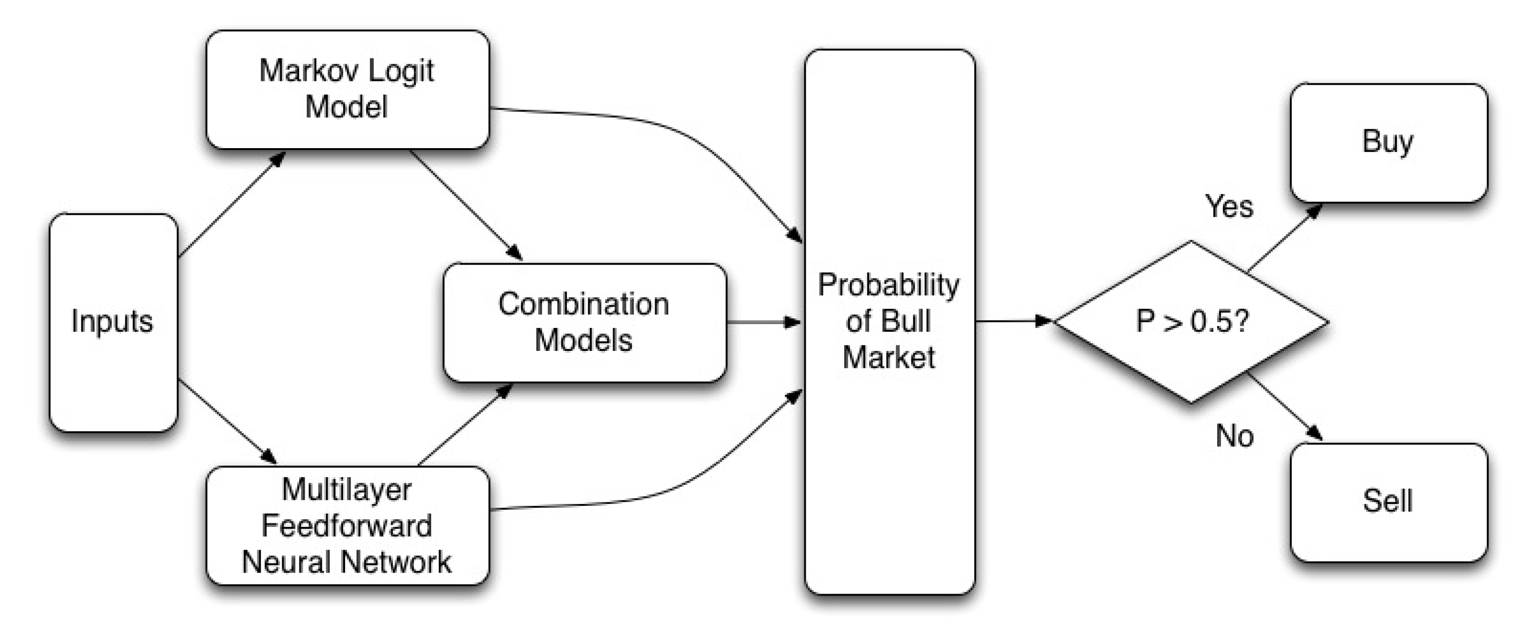
In this section, we first discuss how to use the self-adjusting Markov logit model (ML) and the neural network model (NN) to identify the state of current market cycle, i.e., the bullish or bearish state by carefully assessing the inclusion of variables as inputs. We then discuss two different weighting methods used to derive our combination models, which will be used to predict the macro-cycles of the selected currencies and assess the predicative power and market timing ability of the model. We eventually assess the performance of each individual model and the combination models by comparing their respective trading results. Figure 1 presents the structure of this study. In all the models, the dependent variable will be the state of the current market cycle—whether it is bull or bear. We assign a value of 1 to the bull market and 0 to the bear market, and then include in the study a total of 4 “complex” models, namely, the self-adjusting Markov logit model (ML), the neural network model (NN), the equal weighted combination model (ECM), and the profit-weighted combination model (PCM). We first feed our inputs into the ML and NN models to get predictions for the probability of a bull market, and obtain trading results based on these predictions. Then, we use the ML and NN predictions in the combination models to get predictions of the probability of a bull market, and obtain trading results. Finally, we compare the trading results and assess the model performance.

Our empirical strategy implies three methodological advantages. First, trading longer-term trends (macro-cycles) helps reduce the number of trades required, since we do not adjust trading positions every period. This in turn reduces transaction costs, especially when a large number of orders are placed. Then, a simple moving average crossover rule is adopted in the models that are able to identify the bull and bear macro-cycles in forecasting foreign exchange rates. This rule is widely used by market participants and is viewed as a relatively reliable indicator of market trends. By incorporating this trading rule in the models, we will be able to filter trade orders and identify the bull and bear periods of the market. In particular, the trading strategy is designed in such a way that the investment decision is conditional on trading signals estimated from the models. Finally, with this method we will be able to trade at higher frequency if required and reduce noise by trading macro-cycles.

3.1. Parametric Self-Adjusting Markov Logistic Model

We assume that the fundamental macroeconomic variables have a different effect on the bullish market and bearish market, and such effect on the probability of a future market state depends on the current state. We set the following Markov logit regression model to reflect these effects on the probability of a bullish market state:

$${\pi }_{qt}=\mathrm{Pr}\left[S_t=u|S_{t-1}=q,x_{t-1}\right]=f\left({\beta }_q^{\prime }·x_{t-1}\right)=f\left(z\right)$$

(1)

where ${\pi }_{qt}$ is the probability of the market state at time t, $q = u,d$, where u denotes a bull market and d denotes a bear market, and $S_t$ represents the state of the market at time $t$; $x_{t-1}$ represents the vector of lagged explanatory variables, with the first term being a constant to capture the intercept term; ${\beta }_q$ is the coefficient vector to capture the time varying effects of the explanatory variables in different states; and $f$ represents the logistic function. We define a bull market if the probability of a bull market is larger than 0.5, and otherwise a bear market, namely,

$$\begin{array}{c}If {\pi }_{qt+1}>0.5, predicted state=bull, S_{t+1}=1\hfill \\ If {\pi }_{qt+1}\le 0.5, predicted state=bear, S_{t+1}=0\hfill \end{array}$$

The different market status will then determine the corresponding investment strategy, which is used to assess the predictive accuracy performance of the models. The variable z in Equation (1) is defined as:

$$z={\beta }_{d0}+{\beta }_{u0}{D}_0+{\beta }_{d1}{X}_{1,t-1}+{\beta }_{u1}{D}_1{X}_{1,t-1}+B_{d2}{X}_{2,t-1}+{\beta }_{u2}{D}_2{X}_{2,t-1}+\cdots +{\beta }_{dk}{X}_{k,t-1}+{\beta }_{uk}{D}_k{X}_{k,t-1}+{\epsilon }_t$$

(2)

where $D_k$ is a dummy variable that is equal to 1 if the previous state is a bull market and 0 if the previous state is a bear market. Thus, the coefficient for a particular variable $X_{k,t-1}$ is the summation of the coefficients on $X_{k,t-1}$ and $D_k{X}_{k,t-1}$, and the coefficient for the same variable in a bear market is just the coefficient on $X_{k,t-1}$. ${\epsilon }_t$ is the error term.

To determine which variables need to be included in a model, we often have to balance model bias and variance, as too many variables included will lower the precision of the estimates and too few variables will lead to biased results. In this study, we repeatedly estimate the logit model with different combinations of fundamental macroeconomic variables to choose the specification with the lowest AIC. The variables finally included in the empirical study are the interest rate differentials, relative price level, relative money supply, and real income, as well as the stock return differentials and oil returns.

3.2. Multilayer Feed-Forward Neural Network

Recent studies have shown that ANNs, as a powerful statistical prediction and system modeling technique, can approximate any continuous function and detect the nonlinear patterns of the underlying functional relationships. In comparison with other classes of nonlinear models, ANNs have the advantage of approximating a large class of functions with a high degree of accuracy and without a priori assumptions about the data (see, for instance, [46,49,50,51,52]), and are also more effective at describing the dynamics of non-stationary time series due to its unique non-parametric and non-assumable properties. ANNs also have the ability to generalize, and adequately infer the unseen part of a population even when the sample data is noisy. This suggests that ANNs are ideal for forecasting, since forecasting involves inferring the unseen part of the population from past behavior. However, due to their nonparametric nature, neural networks are often considered black boxes, and the exact relationships can be tough or almost impossible to extract from the trained model.

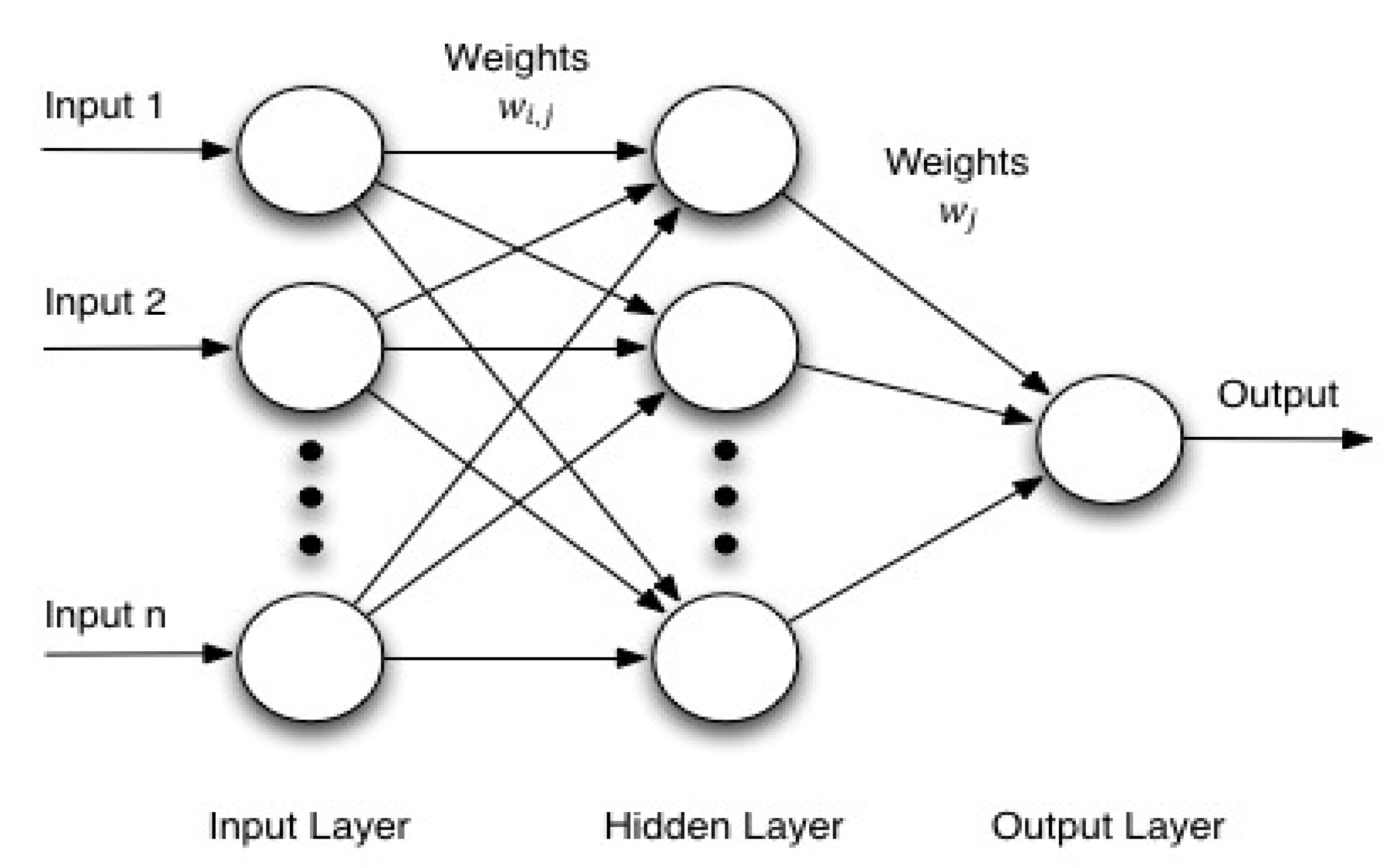
In this study, we intend to use a multilayer feedforward neural network to classify bull or bear market cycles. As illustrated in Figure 2, the ANN model consists of an input layer, hidden layer and output layer. The hidden layers can capture the nonlinear relationship between variables. Each layer communicates with the next layer through a weight connection network, which makes the networks capable to capture relatively complex phenomena.

To estimate the probability of the next state being in a bull market cycle, we specify the ANN model as follows:

$${\pi }_{t,NN}=w_0+{\displaystyle \sum }_{j=1}^q{w}_j*g\left(w_{0,j}+{\displaystyle \sum }_{i=1}^p{w}_{i,j}*x_i\right)+{\epsilon }_t$$

(3)

where $q$ is the number of units in the hidden layer, $p$ is the number of input variables, $g$ is the logistic function, $w_{i,j}\left(i=0,1,2,\dots ,p, j=1,2,\dots ,q\right)$ denotes a matrix of coefficients from the input-layer units to the hidden-layer units, $w_j\left(j=0,1,2,\dots ,q\right)$ is a vector of coefficients from the hidden-layer units to the output-layer units, $x_i$ represents a matrix of input variables, and ${\epsilon }_t$ is the error term. The parameters are estimated by minimizing the sum of squared errors, ${{\displaystyle \sum }}^{ }{\epsilon }_t{}^2.$ We pick small random values as initial weights of the neural network. If the outputs are optimal, the process will halt, and if not, the weights are adjusted, and the process will continue until an optimal solution is found. We use the Levenberg–Marquardt algorithm for estimation because it is the fastest algorithm for moderate-sized feedforward neural networks. The choice of $q$ is data-dependent, and there is no systematic rule in deciding this parameter. In our estimations, we found that $q=10$ gives us the best predictive performance, and hence we hold this parameter in our estimations.

3.3. Composite Models

There are different methods in determining the weights used in the combined forecasts. In this study, we respectively use the equal weights approach and the profit weighted approach to derive the composite models. The equal weights approach uses an arithmetic average of the individual forecasts respectively from the ML model and the ANN model as the weight to derive the composite model. We specify the equal weights composite model (ECM) as follows:

$${\pi }_{t,ECM}=1/2*{\pi }_{t,ML}+1/2*{\pi }_{t,NN}$$

(4)

where ${\pi }_{t,ML}$ and ${\pi }_{t,NN}$ are the probability of a bull market using both the ML and ANN models. We then construct the profit weighted composite model (PCM) by varying the weights assigned for each individual forecast associated with the ML and ANN models, based on the average amount of profits generated in the last 8-week period. We define the average amount of profits generated in the previous 8-week period and the weight for the ML model, respectively, using Equations (5) and (6),

$$P_{ML,NN}={\displaystyle \sum }_{i=0}^7{r}_{t-i,ML,NN}/8$$

(5)

$$w_{ML}=P_{ML}/\left(P_{ML}+P_{NN}\right)$$

(6)

where P_ML and P_NN are the profits generated from the ML model and ANN model, respectively. If either $P_{ML}$ or $P_{NN}$ is negative, $P_{ML,NN}=0$. If both are negative, the model with lesser negative average return will have a higher weight. The final form of the PCM is specified as:

$${\pi }_{t,PCM}=w_{ML}*{\pi }_{t,ML}+\left(1-w_{ML}\right)*{\pi }_{t,NN}$$

(7)

4. Data and Empirical Analysis

4.1. Data Description

In this study, we use three pairs of weekly exchange rates, including the US dollar (USD), the Japanese yen (JPY) and the Canadian dollar (CAD), obtained from Datastream. To make this study methodologically comparable with existing studies [19,39,46,49,53] and to demonstrate the superior performance of our unique hybrid forecast model, we deliberately limit the sample spanning from 1 January 1993 to 25 January 2013. As we are more concerned about the longer-term cycles of the currency-pair movements, the weekly exchange rates will allow us to better manage the sample size issue than the monthly data, and also have not much unnecessary noise as with the daily data. We take the exchange rates at the end of the week in our study.

With respect to the macroeconomic variables, following [40,54], we use 10-year government bond and 3-month treasury bill differentials, year over year (YoY) CPI growth differentials, YoY M1 growth differentials and YoY industrial production growth respectively to proxy the interest rate differentials, relative price level, relative money supply and relative real income in the popular monetary model. As Japan does not have 3-month treasury bills, we use the Japanese Interbank 3-month rate provided by the British Bankers’ Association. In addition, following [39], we also include oil prices as one of our input variables. Canada is the sixth largest oil-producing country in the world, and the largest single source of oil imports into the United States. More effect is expected from the oil prices changes onto the exchange rate. Although there is inconclusive and mixed evidence of correlation between stock markets and foreign exchange markets [55,56,57,58,59,60], we include stock market returns in our empirical study which are proxied by the S&P500, Nikkei, and S&P/TSX Composite indexes, respectively.

Before proceeding to the model estimations, we employed the augmented Dickey-Fuller (ADF) and the Efficient Modified Phillips-Perron (PP) tests to check the stationarity of all the series. Our findings, available upon request, show that all ADF and PP test statistics are significant at the 1% level, thereby indicating that all the return series are stationary.

4.2. Empirical Results

Our estimation strategy proceeds as follows: we begin with model estimations and forecasting to assess the predictive accuracy of the two models based on the estimated bull or bear market states, and then compare the investment strategy and performance associated with the estimated market states of each model. For comparison purpose, we develop a benchmark model corresponding to simply buying/selling the currency pair when the price of the exchange rate becomes higher/lower than the simple moving average (SMA). The SMA for each currency pair is calculated as follows:

$$SM{A}_{n,t}=({\displaystyle \sum }_{i=0}^{n-1}{P}_{t-i})/n$$

where $SM{A}_{n,t}$ is the $n$-period simple moving average at time $t$. A bull market occurs when the currency pair price just crosses the SMA and becomes greater than the SMA. A bear market occurs when the currency pair price crosses the SMA and becomes smaller than the SMA. In this study, we use both the 50 and 100 SMA. Finally, we assess the market timing ability of both the ECM and the PCM, and test the significance of the macroeconomic variables in forecasting the foreign exchange rates.

Table 1. Classification statistics for all currency pairs.

	USD/CAD				USD/JPY				CAD/JPY
	50-SMA		100-SMA		50-SMA		100-SMA		50-SMA		100-SMA
	Bull	Bear	Bull	Bear	Bull	Bear	Bull	Bear	Bull	Bear	Bull	Bear
No. of cycles	31	31	30	30	36	37	27	28	36	36	26	26
Mean (% change per week)	0.24	−0.26	0.20	−0.21	0.40	−0.51	0.29	−0.46	0.39	−0.50	0.21	−0.49
Volatility (%)	1.18	1.04	1.14	1.09	1.60	2.19	1.63	2.26	1.59	2.22	1.64	2.45
Average Period	14.58	17.10	14.53	18.20	13.03	16.08	15.52	23.30	15.17	12.11	26.19	11.58
Median Period	6.00	11.00	5.00	5.50	6.00	8.00	4.00	8.00	8.00	5.50	7.50	4.00
Standard Deviation of Period	17.60	17.12	21.69	34.89	15.13	19.47	25.43	40.40	19.45	14.88	51.12	15.07
Probability of Persistence	0.931	0.942	0.931	0.945	0.938	0.921	0.957	0.933	0.934	0.917	0.962	0.914
Unconditional Probability	0.460	0.540	0.444	0.556	0.552	0.448	0.600	0.400	0.556	0.444	0.693	0.307

displays the summary statistics of the exchange rates and the number of classified bull and bear markets based on the SMA criteria. We note from Table 1 that the 100-SMA generally has fewer bull and bear cycles than the 50 SMA, and also has higher probability of persistence of state in most cases. Given this feature, it is expected that the predictive accuracy of the benchmark model should be better than other non-SMA models, and, for the same reason, the ML and the combination models should outperform other non-SMA model as the former two are based on the benchmark model. However, this might also mean that these models are less sensitive to changes in the market, which would affect their investment performance.

It is noted in Table 1 that, although the exchange rates of both USD/JPY and CAD/JPY have more cycles and shorter average periods for 50-SMA and less cycles for 100-SMA than that of the USD/CAD, the volatility of the USD/CAD is much smaller than that for USD/JPY and CAD/JPY. The persistent regime switching of these two exchange rates would be a consequence of the increased volatility of USD/JPY and CAD/JPY, and this may adversely affect predictive accuracy performance. However, the frequent regime switching may also increase sensitivity to changes in price, hence boosting investment performance. It is also noted that the unconditional probability of the bull market is larger than that of the bear periods for USD/JPY and CAD/JPY, and vice versa for USD/CAD.

We now turn to the discussion of predictive accuracy. We estimate the models to determine the predictive accuracy of the bull/bear market states in terms of the percentage of bull/bear states that the model predicts correctly. We compare directional accuracy of each model, which is critical to successful trading. The first two-thirds of the data are used to perform the initial regression and training of the neural network, and the rest of the data are used to check for the predictive accuracy of the models and for out-of-sample forecasting. We also conduct the Pesaran–Timmermann (PT) [61] predictive failure test to determine the prediction power of a model.

Table 2. Predictive accuracy of various models.

USD/CAD: 50 SMA
	In-Sample (Bull:95/Bear: 69)					Out-of-Sample (Bull:41/Bear: 123)
	ML	BM	NN	ECM	PCM	ML	BM	NN	ECM	PCM
% Bull Correct	46.32	52.63	93.68	48.42	72.63	21.95	21.95	92.68	21.95	53.66
% Bear Correct	76.81	63.77	7.25	72.46	60.87	67.48	67.48	4.07	65.85	63.41
DA (%)	59.15	57.32	57.32	58.54	67.68	56.10	56.10	26.22	54.88	60.98
Buy-hold %	57.93	57.93	57.93	57.93	57.93	25.00	25.00	25.00	25.00	25.00
PT-test Stat	3.04 ***	2.09 **	0.24	2.71 ***	4.31 ***	−1.28	−1.28	−0.84	−1.47	1.93 **
USD/CAD: 100 SMA
	In-Sample (Bull:96/Bear:68)					Out-of-Sample (Bull:32/Bear: 132)
	ML	BM	NN	ECM	PCM	ML	BM	NN	ECM	PCM
% Bull Correct	39.58	27.08	45.83	38.54	48.96	21.88	21.88	3.13	21.88	21.88
% Bear Correct	82.35	52.94	80.88	82.35	82.35	84.85	84.85	97.73	84.85	87.88
DA (%)	57.32	37.80	60.37	56.71	62.80	72.56	72.56	79.27	72.56	75.00
Buy-hold %	58.54	58.54	58.54	58.54	58.54	19.51	19.51	19.51	19.51	19.51
PT-test Stat	3.02 ***	−2.64	3.55 ***	2.89 ***	4.13 ***	0.92	0.92	0.28	0.92	1.43 *
USD/JPY: 50 SMA
	In-Sample (Bull:86/Bear:89)					Out-of-Sample (Bull:93/Bear:82)
	ML	BM	NN	ECM	PCM	ML	BM	NN	ECM	PCM
% Bull Correct	63.95	63.95	93.02	63.95	81.40	45.16	45.16	95.70	45.16	70.97
% Bear Correct	66.29	66.29	19.10	66.29	48.31	53.66	41.46	17.07	52.44	51.22
DA (%)	65.14	65.14	55.43	65.14	64.57	49.14	43.43	58.86	48.57	61.71
Buy-hold %	49.14	49.14	49.14	49.14	49.14	53.14	53.14	53.14	53.14	53.14
PT-test Stat	4.01 ***	4.01 ***	2.38 ***	4.01 ***	4.17 ***	−0.16	−1.77	2.78 ***	−0.32	3.01 ***
USD/JPY: 100 SMA
	In-Sample (Bull:115/Bear:60)					Out-of-Sample (Bull:106/Bear:69)
	ML	BM	NN	ECM	PCM	ML	BM	NN	ECM	PCM
% Bull Correct	68.70	68.70	73.91	68.70	90.43	38.68	23.58	83.02	37.74	66.98
% Bear Correct	80.00	80.00	53.33	80.00	88.33	59.42	59.42	27.54	59.42	59.42
DA (%)	72.57	72.57	66.86	72.57	89.71	46.86	37.71	61.14	46.29	64.00
Buy-hold %	65.71	65.71	65.71	65.71	65.71	60.57	60.57	60.57	60.57	60.57
PT-test Stat	6.14 ***	6.14 ***	3.59 ***	6.14 ***	10.30 ***	−0.25	−2.40	1.68	−0.38	3.45 ***
CAD/JPY: 50 SMA
	In-Sample (Bull:77/Bear:87)					Out-of-Sample (Bull:80/Bear:84)
	ML	BM	NN	ECM	PCM	ML	BM	NN	ECM	PCM
% Bull Correct	59.74	59.74	64.94	55.84	63.64	36.25	36.25	76.25	20.00	60.00
% Bear Correct	67.82	67.82	55.17	67.82	59.77	54.76	40.48	22.62	66.67	54.76
DA (%)	64.02	64.02	59.76	62.20	61.59	45.73	38.41	48.78	43.90	57.32
Buy-hold %	46.95	46.95	46.95	46.95	46.95	48.78	48.78	48.78	48.78	48.78
PT-test Stat	3.55 ***	3.55 ***	2.59 ***	3.06 ***	3.00 ***	−1.17	−2.99	−0.17	−1.93	1.90 **
CAD/JPY: 100 SMA
	In-Sample (Bull:104/Bear:60)					Out-of-Sample (Bull:94/Bear: 70)
	ML	BM	NN	ECM	PCM	ML	BM	NN	ECM	PCM
% Bull Correct	82.69	67.31	87.50	98.08	97.12	32.98	13.83	100.00	67.02	67.02
% Bear Correct	76.67	80.00	41.67	70.00	76.67	60.00	60.00	0.00	25.71	52.86
DA (%)	80.49	71.95	70.73	87.80	89.63	44.51	33.54	57.32	49.39	60.98
Buy-hold %	63.41	63.41	63.41	63.41	63.41	57.32	57.32	57.32	57.32	57.32
PT-test Stat	7.53 ***	5.85 ***	4.28 ***	9.51 ***	9.97 ***	−0.93	−3.84	Inf	−1.01	2.56 ***

Note: The PT-test is a Hausman-type test designed to assess the performance of sign predictions, with the assumption that the distributions of the actual state and predictor are continuous, independent and invariant over time. We do not use RMSE, as it is inappropriate to compare RMSE for a binary model. The table reports the predictive accuracy of the Markov Logit (ML), benchmark (BM), neural network (NN), equal weighted combination (ECM), and profit weighted combination models (PCM). The bracketed numbers indicate the quantity of bull and bear periods in the sample. The numbers in bold indicate the best performance of the 5 models for the particular category. DA refers to the directional accuracy statistic. PT-test refers to the Pesaran–Timmermann predictive failure test, and its critical values at the 1%, 5%, 10% levels are 2.33, 1.645 and 1.282, respectively. ***, ** and * indicate significance at the 1%, 5%, 10% level.

reports the predictive accuracy statistics.

As can be seen in Table 2, the predictive accuracy of the models for USD/CAD is found to be generally higher than others across the board due to the low number of cycle switches, and the directional accuracy for 100-SMA is also better than for 50-SMA. We observe that across both classification methods the complex models outperform the benchmark model. With the exception of the NN model for 50-SMA, all complex models have significant market-timing ability for in-sample validation periods, according to the PT-test. However, for forecasting, it is found that only the PCM model has significant predictive power across all the classification methods. In terms of consistency, the PCM model seems to perform the best under all circumstances. It is interesting to note that, although the PCM model did not achieve the best directional accuracy statistic (DA) for the 100-SMA classification during out-of-sample forecasting, it is still the only model that has significant predictive power according to the PT-test. This is because the PT-test does not simply depend on directional accuracy, but also takes into account the probability of a model making the right classification. In this case, there are more bear periods than bull periods (132 vs. 22). Hence, a model that can correctly predict more bull periods would have more predictive power over a model that simply predicts bears all the time.

For the USD/JPY, it is noted in Table 2 that, largely due to the number of cycle changes, the overall predictive accuracy of the models is poorer than in the case of USD/CAD. Overall, the models seem perform better for the 100-SMA than for the 50-SMA during both the in-sample and out-sample periods, due to its inherent advantage with the exception of the DA scores for out-of-sample forecasting. This suggests that the complex models using 50-SMA can outperform the model with 100-SMA in out-of-sample forecasting despite of the latter’s low volatility advantage. In comparison, the ML model has the best in-sample performance in terms of directional accuracy for 50-SMA, while the PCM performs the best for out-of-sample forecasting. It is also noted that, although most models have significant predictive power for in-sample performance according to the PT-test, the PCM and NN models are the only two models showing a significant predictive ability for out-of-sample forecasting. Based on the PT-test and DA scores, our results suggest that, out of the five models, the PCM is likely the best for out-of-sample forecasting. Similar findings are obtained for CAD/JPY where the PCM model apparently outperform the rest of the models in both 50 SMA and 100 SMA, with the DA being the highest for out-of-sample forecasting in both cases, though all the models have a significant predictive power for in-sample forecasting.

We now turn to the analysis of investment performance of these models with different trading rules. The investment strategy is made such that an investor will take a long position if the model predicts a bull market state in the next period and take a short position if the predicted bull market state changes, and vice versa for a predicted bear market. We then calculate the average weekly return, continuous compounding returns and the annualized return for each investment strategy in both 50 SMA and 100 SMA for each model.

Table 3. Investment performance for various models.

USD/CAD: 50-SMA
	In-Sample						Out-of-Sample
	ML	BM	NN	ECM	PCM	B&H	ML	BM	NN	ECM	PCM	B&H
Annualized Return	4.37%	10.42%	−0.15%	1.71%	5.78%	−0.64%	5.59%	5.59%	−3.32%	6.68%	3.11%	−2.99%
Volatility	13.01%	12.94%	13.03%	13.02%	13.00%	13.03%	9.53%	9.53%	9.56%	9.52%	9.56%	9.56%
Sharpe Ratio	0.34	0.80	−0.01	0.13	0.44	−0.05	0.59	0.59	−0.35	0.70	0.33	−0.31
Cumulative Returns	13.80%	32.86%	−0.48%	5.38%	18.24%	−2.02%	17.64%	17.64%	−10.48%	21.08%	9.82%	−9.42%
Max Weekly Profit	5.22%	8.03%	8.03%	5.22%	8.03%	8.03%	4.99%	4.99%	4.99%	4.99%	4.99%	4.99%
Max Weekly Loss	−2.93%	−2.93%	−3.53%	−2.93%	−3.09%	−3.53%	−2.93%	−2.93%	−3.53%	−2.93%	−3.09%	−3.53%
Max Drawdown	−21.94%	−11.71%	−23.66%	−25.91%	−17.79%	−23.66%	−8.05%	−8.05%	−20.87%	−8.05%	−9.76%	−14.36%
USD/CAD: 100-SMA
	In-Sample						Out-of-Sample
	ML	BM	NN	ECM	PCM	B&H	ML	BM	NN	ECM	PCM	B&H
Annualized Return	19.01%	9.31%	17.10%	17.51%	16.50%	−0.64%	8.26%	8.26%	2.30%	8.26%	9.69%	−2.99%
Volatility	12.75%	12.96%	12.81%	12.80%	12.82%	13.03%	9.50%	9.50%	9.56%	9.50%	9.47%	9.56%
Sharpe Ratio	1.49	0.72	1.34	1.37	1.29	−0.05	0.87	0.87	0.24	0.87	1.02	−0.31
Cumulative Returns	59.95%	29.37%	53.94%	55.22%	52.05%	−2.02%	26.04%	26.04%	7.24%	26.04%	30.55%	−9.42%
Max Weekly Profit	8.03%	8.03%	8.03%	8.03%	8.03%	8.03%	4.99%	4.99%	3.53%	4.99%	4.99%	4.99%
Max Weekly Loss	−2.90%	−2.90%	−4.99%	−2.90%	−2.90%	−3.53%	−2.90%	−2.90%	−4.99%	−2.90%	−2.90%	−3.53%
Max Drawdown	−9.64%	−16.49%	−8.85%	−11.48%	−15.62%	−23.66%	−6.19%	−6.19%	−11.84%	−6.19%	−6.19%	−14.36%
USD/JPY: 50-SMA
	In-Sample						Out-of-Sample
	ML	BM	NN	ECM	PCM	B&H	ML	BM	NN	ECM	PCM	B&H
Annualized Return	20.89%	20.89%	13.18%	20.89%	25.72%	−5.63%	22.14%	21.26%	2.42%	22.95%	20.95%	2.24%
Volatility	19.26%	19.26%	19.40%	19.26%	19.15%	19.47%	13.81%	13.84%	14.15%	13.79%	13.85%	14.15%
Sharpe Ratio	1.08	1.08	0.68	1.08	1.34	−0.29	1.60	1.54	0.17	1.66	1.51	0.16
Cumulative Returns	70.31%	70.31%	44.36%	70.31%	86.56%	−18.96%	74.51%	71.56%	8.14%	77.22%	70.50%	7.54%
Max Weekly Profit	15.28%	15.28%	15.28%	15.28%	15.28%	9.50%	5.28%	5.28%	5.08%	5.28%	5.28%	5.08%
Max Weekly Loss	−4.93%	−5.07%	−5.28%	−4.93%	−5.07%	−5.28%	−4.93%	−5.07%	−5.28%	−4.93%	−5.07%	−5.28%
Max Drawdown	−17.25%	−17.25%	−16.64%	−17.25%	−11.45%	−53.32%	−6.92%	−6.92%	−21.37%	−6.92%	−10.98%	−24.86%
USD/JPY: 100-SMA
	In-Sample						Out-of-Sample
	ML	BM	NN	ECM	PCM	B&H	ML	BM	NN	ECM	PCM	B&H
Annualized Return	9.16%	9.16%	−12.84%	9.16%	9.55%	−5.63%	14.98%	12.15%	3.69%	14.17%	14.51%	2.24%
Volatility	19.44%	19.44%	19.40%	19.44%	19.44%	19.47%	14.00%	14.05%	14.14%	14.01%	14.01%	14.15%
Sharpe Ratio	0.47	0.47	−0.66	0.47	0.49	−0.29	1.07	0.86	0.26	1.01	1.04	0.16
Cumulative Returns	30.82%	30.82%	−43.22%	30.82%	32.12%	−18.96%	50.40%	40.89%	12.41%	47.69%	48.82%	7.54%
Max Weekly Profit	15.28%	15.28%	9.50%	15.28%	15.28%	9.50%	5.28%	5.28%	5.28%	5.28%	5.28%	5.08%
Max Weekly Loss	−5.07%	−4.93%	−5.07%	−5.07%	−5.07%	−5.28%	−5.07%	−4.93%	−5.07%	−5.07%	−5.07%	−5.28%
Max Drawdown	−22.46%	−22.46%	−58.39%	−22.46%	−22.26%	−53.32%	−10.23%	−10.23%	−22.76%	−10.23%	−10.94%	−24.86%
CAD/JPY: 50-SMA
	In-Sample						Out-of-Sample
	ML	Benchmark	NN	ECM	PCM	B&H	ML	Benchmark	NN	ECM	PCM	B&H
Annualized Return	22.69%	22.69%	15.83%	24.45%	22.23%	−5.62%	20.08%	18.03%	5.24%	20.97%	21.35%	−2.27%
Volatility	19.72%	19.72%	19.85%	19.68%	19.73%	19.96%	13.99%	14.05%	14.25%	13.97%	13.96%	14.26%
Sharpe Ratio	1.15	1.15	0.80	1.24	1.13	−0.28	1.43	1.28	0.37	1.50	1.53	−0.16
Cumulative Returns	71.55%	71.55%	49.92%	77.11%	70.10%	−17.73%	63.32%	56.87%	16.53%	66.14%	67.35%	−7.15%
Max Weekly Profit	15.28%	15.28%	15.28%	15.28%	15.28%	9.50%	5.28%	5.28%	5.08%	5.28%	5.28%	5.08%
Max Weekly Loss	−4.93%	−5.07%	−5.28%	−4.93%	−5.07%	−5.28%	−4.93%	−5.07%	−5.28%	−4.93%	−5.07%	−5.28%
Max Drawdown	−17.25%	−17.25%	−27.62%	−20.12%	−19.28%	−53.32%	−6.92%	−6.92%	−20.48%	−6.92%	−7.30%	−24.86%
CAD/JPY: 100-SMA
	In-Sample						Out-of-Sample
	ML	Benchmark	NN	ECM	PCM	B&H	ML	Benchmark	NN	ECM	PCM	B&H
Annualized Return	1.77%	9.05%	7.37%	14.15%	21.51%	−5.62%	13.61%	9.46%	−2.27%	12.45%	13.82%	−2.27%
Volatility	19.97%	19.94%	19.95%	19.88%	19.75%	19.96%	14.14%	14.21%	14.26%	14.16%	14.14%	14.26%
Sharpe Ratio	0.09	0.45	0.37	0.71	1.09	−0.28	0.96	0.67	−0.16	0.88	0.98	−0.16
Cumulative Returns	5.59%	28.56%	23.24%	44.62%	67.84%	−17.73%	42.91%	29.85%	−7.15%	39.27%	43.59%	−7.15%
Max Weekly Profit	15.28%	15.28%	12.57%	15.28%	15.28%	9.50%	5.28%	5.28%	5.08%	5.08%	5.28%	5.08%
Max Weekly Loss	−5.07%	−4.93%	−5.28%	−5.28%	−5.07%	−5.28%	−5.07%	−4.93%	−5.28%	−5.28%	−5.07%	−5.28%
Max Drawdown	−39.72%	−22.46%	−35.41%	−13.99%	−11.20%	−53.32%	−10.23%	−10.23%	−24.86%	−12.46%	−11.87%	−24.86%

Note: The Sharpe Ratio is computed using the mean and standard deviation of the distribution of the final payoff [43]. The maximum drawdown is the maximum loss that has been sustained relative to the highest profit previously attained. Bold numbers indicate the best performance of the 6 models for the particular category.

reports the performance results. In addition, we also calculate the annualized volatility, together with the Sharpe ratio, and report the maximum weekly profits and losses, as well as the maximum drawdown in Table 3.

As can be seen in Table 3, the complex models generally outperform the benchmark model in both in-sample and out-of-sample forecasts, and the PCM outperforms all the other models in terms of annualized and accumulative returns in the out-of-sample forecasting experiment for all the currencies and the trading rules except three cases. For in-sample forecasting, the PCM model performs reasonably well in most cases, although it is not the best in comparison with other models. Overall, it is found that the PCM has a better performance and return for the given risk, judging from the high Sharpe ratio. With respect to the specific currency trading, the results suggest that the ECM model is the most preferred model in out-of-sample forecasting with the 50 SMA trading rules for USD/CAD and USD/JPY, while the PCM model is the best performing model in out-of-sample forecasting with the 100-SMA trading rules. These findings are consistent with those in [18,19].

4.3. Further Investigation

We now turn to the analysis of the market timing ability of the best performing models and the parameter evolution of the ML model to better assess which variables are important through the sample period. In the previous section, we evaluated the forecast performance of the models based on return performance, Sharpe ratio [62], and drawdown over both the in-sample and pseudo out-of-sample period. In this section, we pick the best performing models in forecasting to further investigate their timing ability and returns against the benchmark model as well as the importance of the macroeconomic variables over time.

4.3.1. Market Timing and Cumulative Returns

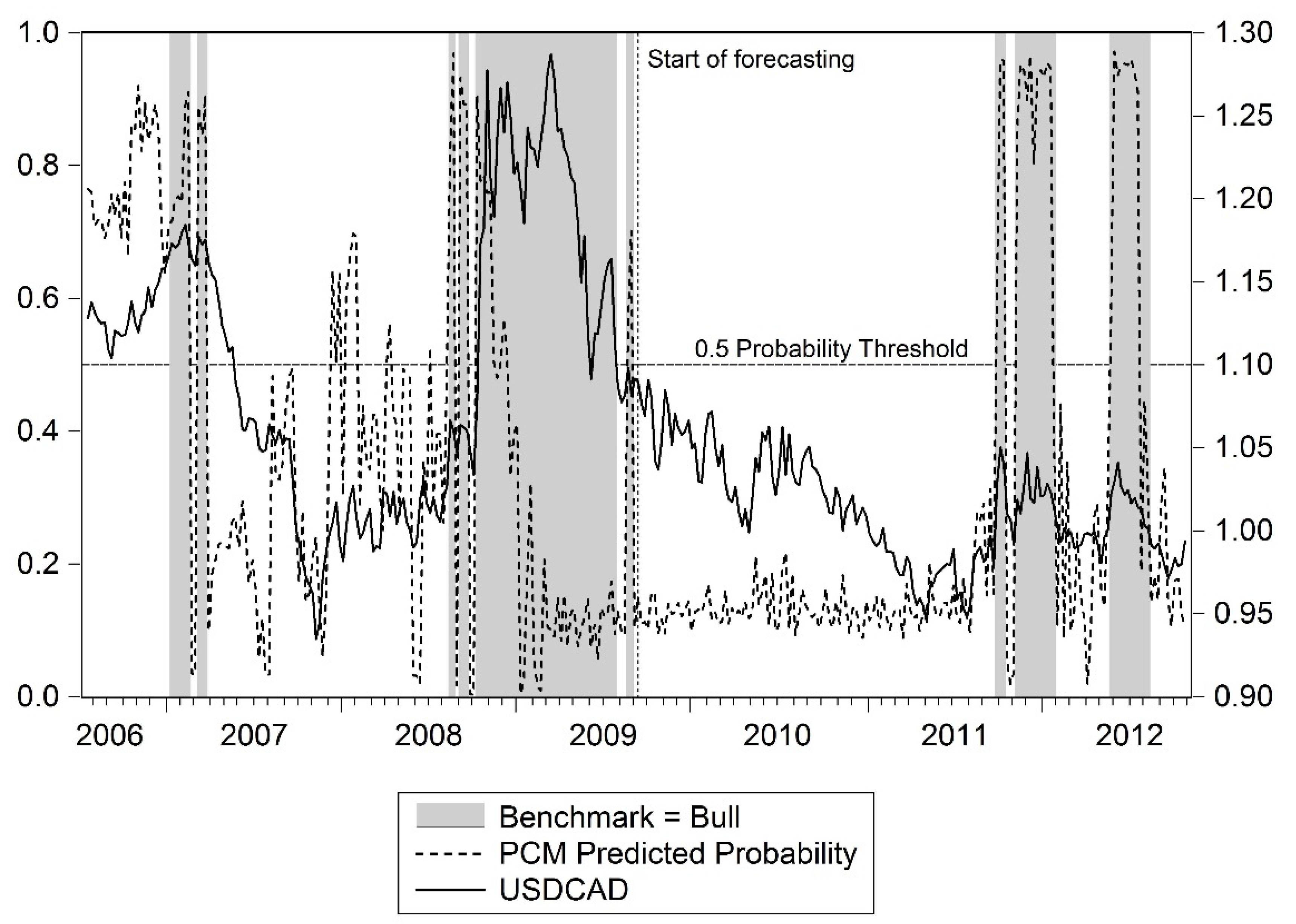
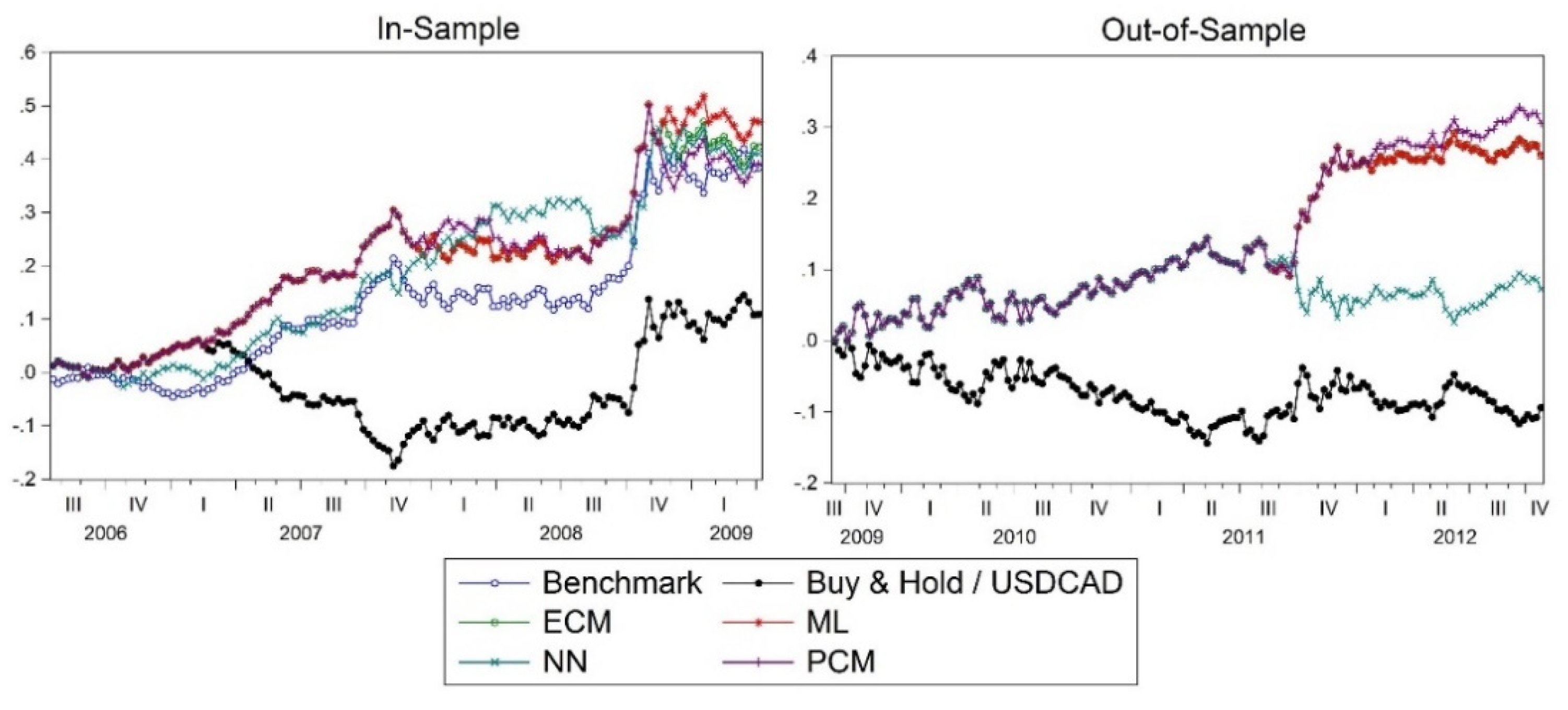
We examine the market timing ability of the PCM model and the benchmark model by applying the 100 SMA trading rules for the three currencies. Figure 3 presents the prediction results of the PCM vs. the benchmark model and the true state for the in-sample and out-of-sample periods for the exchange rate of USD/CAD. It can be seen in Figure 3 that the PCM model correctly predicts a bull market in late 2007, well before the benchmark model for the in-sample period, and again successfully predicts a bear market in late 2008 and early 2009, ahead of the benchmark model or even the actual state. The results confirm the PCM model’s market-timing ability. In the out-of-sample forecasting period, the PCM model also outperforms the benchmark model in predicting the market state changes from bullish to bearish market respectively in 2011 and 2012. These findings further confirm that the PCM model has superior predictive and market-timing abilities and tend to generate high investment return in comparison with the benchmark model. Figure 4 presents the cumulative returns of all the models for trading USD/CAD for both in-sample and out-of-sample periods. As can be seen in Figure 4, the PCM model generates the highest return up to 2008 and again in late 2008 during the in-sample period, and outperforms other models in terms of return through the out-of-sample period. This finding has important implications for investors when considering the choice of models in trading USD/CAD.

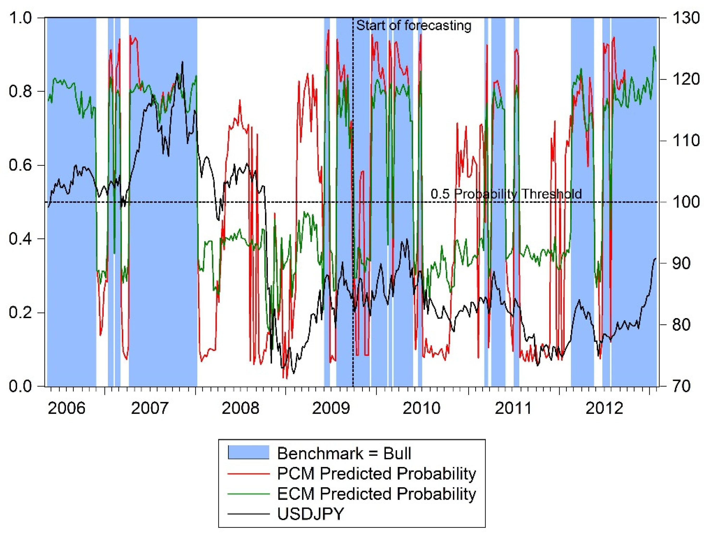
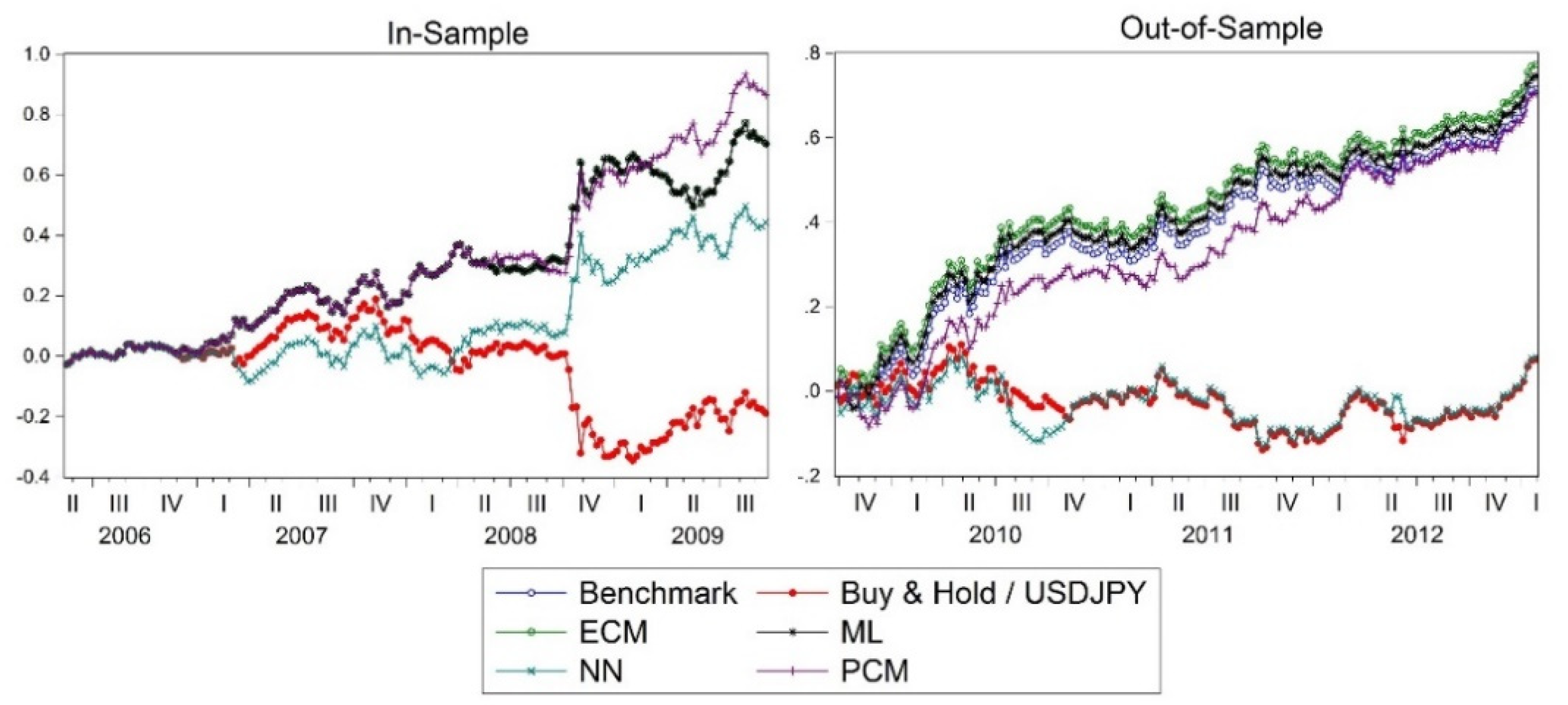
For USD/JPY, we choose both the PCM and ECM models using the 50-SMA trading rules to assess their market-timing abilities as both models are found to be the best performing models. Figure 5 presents the results. As can be seen in Figure 5, the PCM model has the best forecasts on average both over the in-sample and the pseudo out-of-sample period. In particular, it predicts correctly the state changes of the bull and bear markets through 2008 and 2009, and shows a strong market timing ability. Over the pseudo out-of-sample period, although it fails to make a correct prediction in late 2010, the PCM model significantly outperforms the others in predicting the bull market in early 2012. This makes the PCM the most profitable model over the in-sample period and one of the best performers over the pseudo out-of-sample period (Figure 6). That also explains why the PCM has the relatively small maximum drawdown. Overall, all the models except the NN model perform similarly well in the pseudo out-of-sample forecasting, with the ECM model showing a relatively high return in comparison with others (see Figure 6). Most of the models can make a quick adjustment to any changes in market states. Thus, our analysis will focus on the rest of the models, particularly on the PCM model, rather than the NN model.

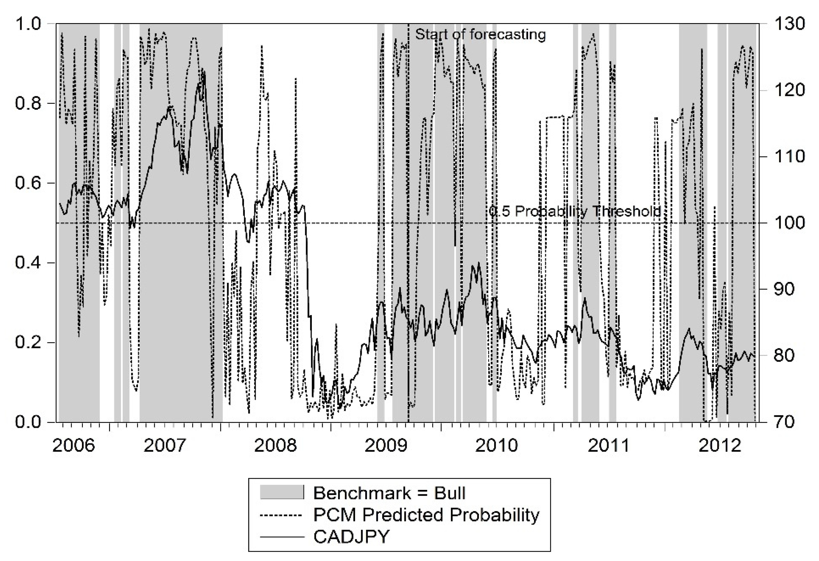
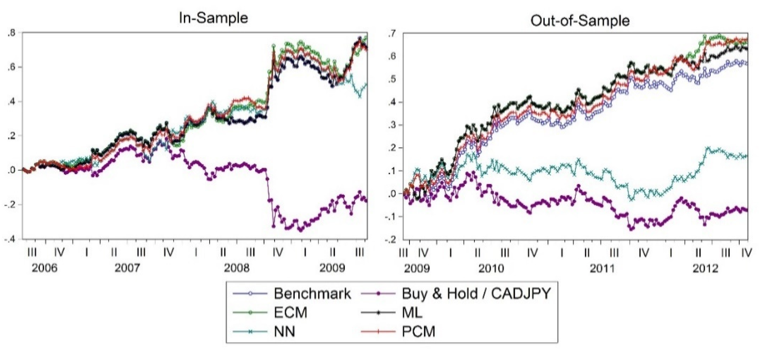
Figure 7 presents the predictive ability of the market states of the PCM model against the benchmark model for CAD/JPY with the 50-SMA trading rules. It can be seen from Figure 7 that the PCM model has a strong predictive ability in detecting a small bull cycle in January 2007 and the bull state in April 2008, while the benchmark model failed during this period. Similarly, when the CAD/JPY exchange rates began to drop in July 2008, the PCM model was able to detect it in a timely fashion, leading to the opposite position in order to profit. The PCM model also correctly predicted a bull market in its early stages in October 2010 ahead of the benchmark model, as well as in November 2012 and April 2012. This further confirms that the PCM model has significant predictive power and market timing ability. The model’s performance in cumulative returns as presented in Figure 8, especially over the pseudo out-of-sample period, lends further support to this finding.

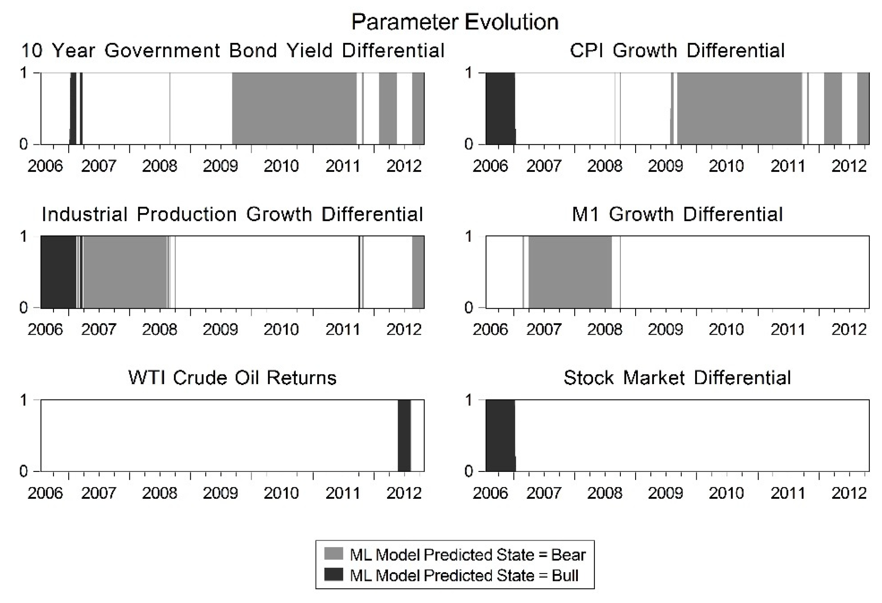
4.3.2. Parameter Evolution in ML Model

In this section, we assess the dynamic changes in importance of the macroeconomic variables in forecasting by employing the parameter evolution analysis. Figure 9 reports the variables which are important through the estimations of the ML model over time incorporating the 100-SMA rules for USD/CAD forecasts. The darker shaded areas indicate that the market state is predicted to be a bull market by the ML model, and the lighter areas are where the model predicts bear. It is found that the 10-year government bond differential and the CPI differential are the most important variables in USD/CAD forecasts, and have been used almost all the time since 2009Q3, especially during bear cycles. This finding has implications for market efficiency and lends support to the interest rate parity and purchasing power parity theories, suggesting that both interest rate and purchasing power parity are widely used by market participants in forecasting exchange rates movement.

In contrast, industrial production and M1 growth appear in forecasting only in the early in-sample period, and have been retained in the model since 2008Q3. As a proxy for GDP growth, the importance of industrial production growth could stem from the fact that a higher GDP growth increases the likelihood of future monetary policy tightening, thereby generating an expectation of future currency appreciation. A rise in capital inflows during the boom time periods also tends to cause the nominal exchange rate to appreciate [53]. The stock market differentials are only used from late 2006 up to 2007, and oil returns appear in the model only in 2012Q2. This finding may come as a surprise, especially when considering a large share of oil exports in Canada. However, it is consistent with the findings in [39] that oil prices were not significant in forecasting exchange rates of longer frequencies.

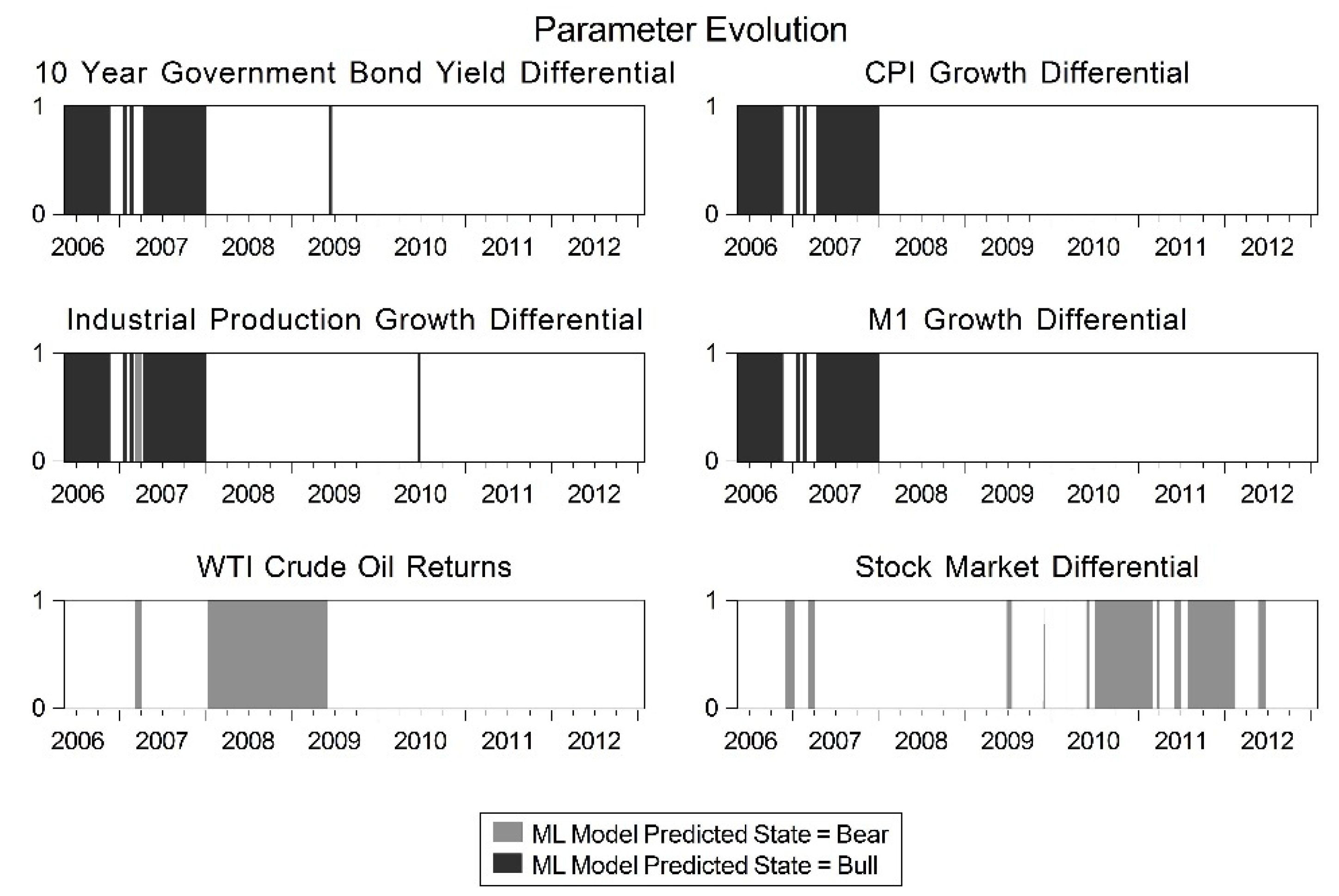
Figure 10 shows the parameter evolution of the ML model for USD/JPY 50-SMA. As can be seen in Figure 10, the government bond, CPI growth, industrial production and M1 growth differentials all appear during the almost identical periods. They are all used in the early in-sample period, from May 2006 to January 2008, and the market is also mostly bullish during this period. However, these variables lose their importance in forecast in the late bear period, while oil returns and stock market differentials appear as the important determinants for USD/JPY forecasts from May 2010 to about May 2012.

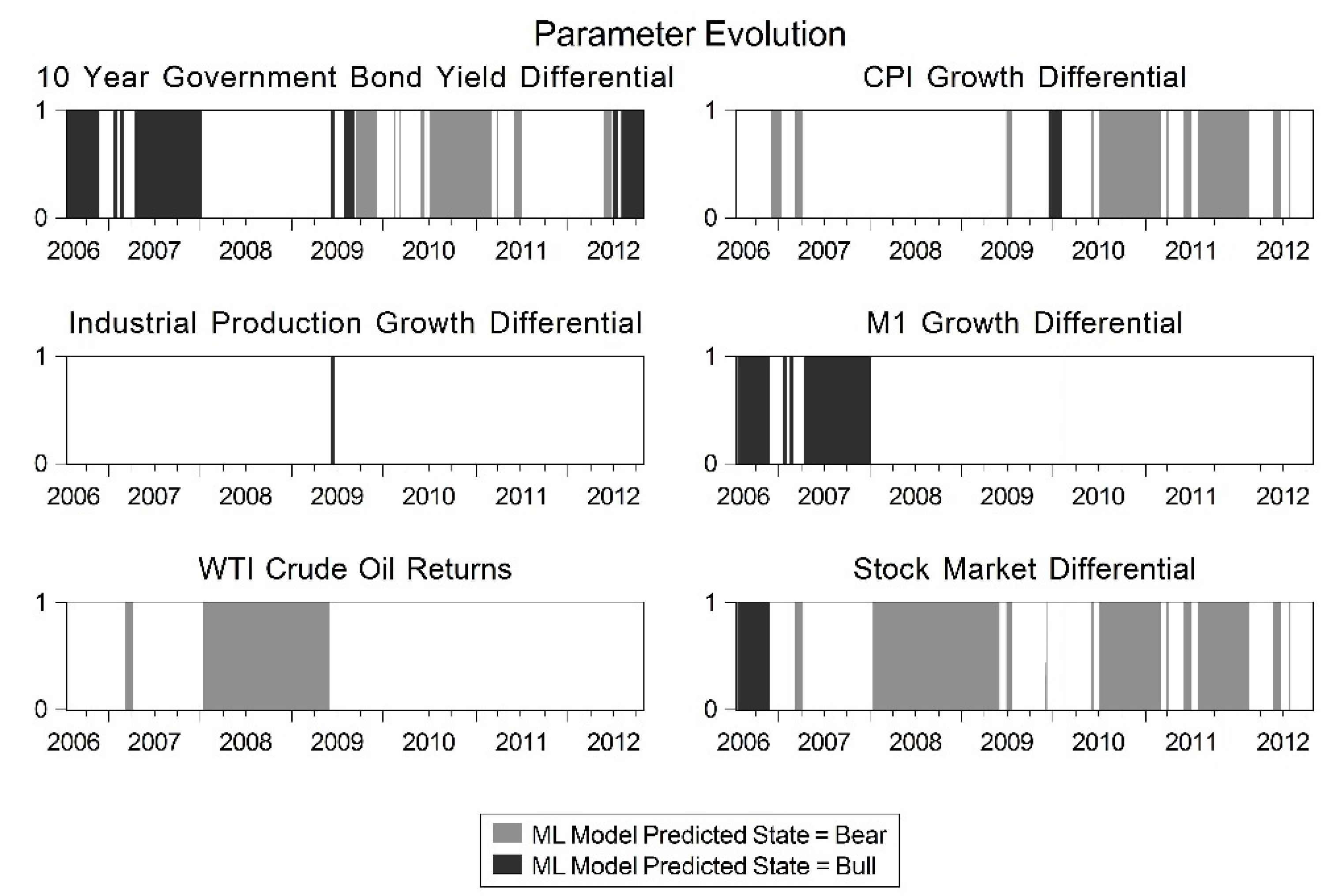
Figure 11 presents how the parameters of the ML model evolve over time for CAD/JPY with the 50-SMA trading rules. It can be seen that the government bond yield, CPI differentials and the stock market returns are the most important variables for CAD/JPY forecasts in most of the time, while the other variables are important only in the early in-sample period. One may note that stock market returns appear to be an important variable in forecasting the exchange rates of both USD/JPY and CAD/JPY, implying that the exchange value of the Japanese yen is influenced very much by how the Japanese stock market performs. This finding lends support to the hotly debated symmetric or asymmetric issues on the price spillover between the two financial markets, and has important implications for market participants regarding decision making in international portfolio and currency risk strategies.

5. Concluding Remarks

Exchange rate forecasts have long been challenging for researchers. The advent of nonlinear non-parametric models in recent years like the neural network model has improved forecasting, but researchers have yet to find a good way of forecasting foreign exchange prices. In contrast to existing studies, this paper aims to forecast market cycles by using the linear and nonlinear models embedded with technical trading rules to determine the best performing model in forecast based on its prediction power and investment performance.

The results show that that using different trading rules in the forecasting models can lead to a big difference in terms of predictive ability and investment performance. The model specification and performance are found sensitive to the different trading rules and currency volatility. It is also found that the PCM model incorporating the 50-SMA trading rule can generate large profits for USD/JPY and CAD/JPY, and similarly for USD/CAD with the 100 SMA rules. The results suggest that the PCM model has significant predictive power and market timing ability, and consistently outperforms any benchmark models in the pseudo out-of-sample forecasting. It is also found that, when the PCM model is used in forecasting, the annualized returns, volatility and maximum drawdown all have been improved in comparison with the single model forecasts. This finding is consistent with many of the existing studies (see for instance [43]). These findings have practical implications in the markets. Traders could use the PCM to predict the major changes in market cycles and adjust their portfolios accordingly. In particular, investment strategy can be made such that an investor will take a long position when the model predicts a bull market state in the subsequent period and take a short position if the predicted bull market state changes, and vice versa for a predicted bear market. Business firms could better hedge their currency risk through early detection of a state change in exchange rate trends.

Despite PCM’s market timing ability and predictive power, the investment performance of the model is found only slightly better than the benchmark model in some cases, especially when government intervention is observed. In such a situation, the study finds that the simple technical trading rules can perform as good as the complex models. This is because in such a situation the market fundamentals become relatively less important due to the manipulation of exchange rates.

With regard to parameter evolution, the results show that the 10-year government bond yield differentials and CPI differentials are the most important factors in exchange rate forecasts in most time periods, suggesting that the interest rate parity and purchasing power parity concepts are applied in trading by the market participants. Stock market differentials were found to be particularly useful in forecasting the Japanese yen currency pairs, possibly due to the yen’s “safe haven” status.

There are some possible limitations to this study. As this study only focuses on single-lag variables, it is possible to consider using multiple lags to improve the prediction power of the models though this will greatly increase the complexity of the system. The AIC can be used to determine the optimal number of lags for each variable. This will be addressed in a future study.

References

- Meese, R.A.; Rogoff, K. Empirical exchange rate models of the seventies: Do they fit out of sample? J. Int. Econ. 1983, 14, 3–24. [Google Scholar] [CrossRef]
- Meese, R.; Rogoff, K.S. The out-of-sample failure of empirical exchange rate models: Sampling error or misspecification? In Exchange Rates and International Macroeconomics; Frenkel, J.A., Ed.; Chicago University of Chicago Press: Chicago, IL, USA, 1982; pp. 1–54. [Google Scholar]
- Cheung, Y.-W.; Chinn, M.D.; Pascual, A.G. Empirical exchange rate models of the nineties: Are any fit to survive? J. Int. Money Financ. 2005, 24, 1150–1175. [Google Scholar] [CrossRef] [Green Version]
- Engel, C.; Mark, N.C.; West, K.D. Exchange rate models are not as bad as you think. In NBER Macroeconomics Annual 2007; Acemoglu, D., Rogoff, K., Woodford, M., Eds.; MIT Press: Cambridge, MA, USA, 2008; pp. 381–441. [Google Scholar]
- Rossi, B. Exchange rate predictability. J. Econ. Lit. 2013, 51, 1063–1119. [Google Scholar] [CrossRef] [Green Version]
- Molodtsova, T.; Papell, D.H. Out-of-sample exchange rate predictability with Taylor rule fundamentals. J. Int. Econ. 2009, 77, 167–180. [Google Scholar] [CrossRef]
- Li, J.; Tsiakas, I.; Wang, W. Predicting Exchange rates out of sample: Can economic fundamentals beat the random walk? J. Financ. Econ. 2014, 13, 293–341. [Google Scholar] [CrossRef] [Green Version]
- Jamali, I.; Yamani, E. Out-of-sample exchange rate predictability in emerging markets: Fundamentals versus technical analysis. J. Int. Financ. Mark. Inst. Money 2019, 61, 241–263. [Google Scholar] [CrossRef]
- Lustig, H.; Verdelhan, A. The cross section of foreign currency risk premia and US consumption growth risk. Am. Econ. Rev. 2007, 97, 89–117. [Google Scholar] [CrossRef] [Green Version]
- Lustig, H.; Roussanov, N.; Verdelhan, A. Common risk factors in currency markets. Rev. Financ. Stud. 2011, 24, 3731–3777. [Google Scholar] [CrossRef]
- Menkhoff, L.; Sarno, L.; Schmeling, M.; Schrimpf, A. Carry trades and global FX volatility. J. Financ. 2012, 67, 681–718. [Google Scholar] [CrossRef] [Green Version]
- Menkhoff, L.; Sarno, L.; Schmeling, M.; Schrimpf, A. Currency momentum strategies. J. Financ. Econ. 2012, 106, 660–684. [Google Scholar] [CrossRef] [Green Version]
- Dahlquist, M.; Hasseltoft, H. Economic momentum and currency returns. J. Financ. Econ. 2020, 136, 152–167. [Google Scholar] [CrossRef] [Green Version]
- Colacito, R.; Riddiough, S.J.; Sarno, L. Business cycles and currency returns. J. Financ. Econ. 2020, 137, 659–678. [Google Scholar] [CrossRef]
- Corte, P.D.; Riddiough, S.J.; Sarno, L. Currency premia and global imbalances. Rev. Financ. Stud. 2016, 29, 2161–2193. [Google Scholar] [CrossRef]
- Brock, V.; Lakonishok, J.; LeBaron, B. Simple technical trading rules and the stochastic properties of stock returns. J. Financ. 1992, 47, 1731–1764. [Google Scholar] [CrossRef]
- Knez, P.J.; Ready, M.J. Estimating the profits from trading strategies. Rev. Financ. Stud. 1996, 9, 1121–1163. [Google Scholar] [CrossRef]
- Gençay, R. Linear, non-linear and essential foreign exchange rate prediction with simple technical trading rules. J. Int. Econ. 1999, 47, 91–107. [Google Scholar] [CrossRef]
- Neely, C.J.; Weller, P.A.; Ulrich, J.M. The adaptive markets hypothesis: Evidence from the foreign exchange market. J. Financ. Quant. Anal. 2009, 44, 467–488. [Google Scholar] [CrossRef] [Green Version]
- Zhu, Y.; Zhou, G. Technical analysis: An asset allocation perspective on the use of moving averages. J. Financ. Econ. 2009, 92, 519–544. [Google Scholar] [CrossRef]
- Shen, X.; Tsui, A.K.; Zhang, Z. Volatility timing in CPF investment funds in Singapore: Do they outperform non-CPF funds? Risks 2019, 7, 106. [Google Scholar] [CrossRef] [Green Version]
- Neely, C.; Weller, P.A. Lessons from the evolution of foreign exchange trading strategies. J. Bank. Financ. 2013, 37, 3783–3798. [Google Scholar] [CrossRef] [Green Version]
- Han, Y.; Yang, K.; Zhou, G. A new anomaly: The cross-sectional profitability of technical analysis. J. Financ. Quant. Anal. 2013, 48, 1433–1461. [Google Scholar] [CrossRef]
- Marshall, B.R.; Nguyen, N.H.; Visaltanachoti, N. Time series momentum and moving average trading rules. Quant. Financ. 2016, 17, 405–421. [Google Scholar] [CrossRef]
- Froot, K.A.; Ramadorai, T. Institutional portfolio flows and international investments. Rev. Financ. Stud. 2008, 21, 937–971. [Google Scholar] [CrossRef] [Green Version]
- Fuertes, A.; Phylaktis, K.; Yan, C. Uncovered equity “disparity” in emerging markets. J. Int. Money Financ. 2019, 98, 102066. [Google Scholar] [CrossRef]
- Gente, K.; Leon-Ledesma, M.A. Does the world real interest rate affect the real exchange rate? The South East Asian experience. J. Int. Trade Econ. Dev. 2006, 15, 441–467. [Google Scholar] [CrossRef]
- Bahmani-Oskooee, M.; Tanku, A. Black market exchange rate, currency substitution and the demand for money in LDCs. Econ. Syst. 2006, 30, 249–263. [Google Scholar] [CrossRef]
- Liew, V.K.-S.; Baharumshah, A.Z.; Puah, C.-H. Monetary model of exchange rate for thailand: Long-run relationship and monetary restrictions. Glob. Econ. Rev. 2009, 38, 385–395. [Google Scholar] [CrossRef]
- Wong, H.T. Real exchange rate misalignment and economic growth in Malaysia. J. Econ. Stud. 2013, 40, 298–313. [Google Scholar] [CrossRef]
- Arghyrou, M.G.; Pourpourides, P. Inflation announcements and asymmetric exchange rate responses. J. Int. Financ. Mark. Inst. Money 2016, 40, 80–84. [Google Scholar] [CrossRef]
- Li, M.; Qin, F.; Zhang, Z. Short-term capital flows, exchange rate expectation and currency internationalization: Evidence from China. J. Risk Financ. Manag. 2021, 14, 223. [Google Scholar] [CrossRef]
- Guo, D. Dynamic volatility trading strategies in the currency option market. Rev. Deriv. Res. 2000, 4, 133–154. [Google Scholar] [CrossRef]
- Zhang, Y.-D.; Wu, L. Stock market prediction of S&P 500 via combination of improved BCO approach and BP neural network. Expert Syst. Appl. 2009, 36, 8849–8854. [Google Scholar]
- Kuan, C.-M.; Liu, T. Forecasting exchange rates using feedforward and recurrent neural networks. J. Appl. Econ. 1995, 10, 347–364. [Google Scholar] [CrossRef] [Green Version]
- Hann, T.H.; Steurer, E. Much ado about nothing? Exchange rate forecasting: Neural networks vs. linear models using monthly and weekly data. Neurocomputing 1996, 10, 323–339. [Google Scholar] [CrossRef]
- El Shazly, M.R.; El Shazly, H.E. Comparing the forecasting performance of neural networks and forward exchange rates. J. Multinatl. Financ. Manag. 1997, 7, 345–356. [Google Scholar] [CrossRef]
- Eng, M.H.; Li, Y.; Wang, Q.-G.; Lee, T.H. Forecast forex with ANN using fundamental data. In Proceedings of the 2008 International Conference on Information Management, Innovation Management and Industrial Engineering, Taipei, Taiwan, 19–21 December 2008; pp. 279–282. [Google Scholar]
- Ferraro, D.; Rossi, B.; Rogoff, K. Can oil prices forecast exchange rates? Econ. Res. Initiat. Duke Work. Pap. 2011, 95, 1–53. [Google Scholar]
- Qi, M.; Wu, Y. Nonlinear prediction of exchange rates with monetary fundamentals. J. Empir. Financ. 2003, 10, 623–640. [Google Scholar] [CrossRef]
- Bilson, J.F. Rational expectations and the exchange rate. In The Economics of Exchange Rates: Selected Studies; Frenkel, J.A., Johnson, H.G., Eds.; Addison-Wesley Publishing: Boston, MA, USA, 1978; pp. 75–96. [Google Scholar]
- Mussa, M. The exchange rate, the balance of payments and the monetary and fiscal policy under a regime of controlled floating. In The Economics of Exchange Rates: Selected Studies; Frenkel, J.A., Johnson, H.G., Eds.; Addison-Wesley Publishing: Boston, MA, USA, 1978; pp. 47–65. [Google Scholar]
- Clemen, R.T. Combining forecasts: A review and annotated bibliography. Int. J. Forecast. 1989, 5, 559–583. [Google Scholar] [CrossRef]
- Khashei, M.; Bijari, M.; Ardali, G.A.R. Improvement of auto-regressive integrated moving average models using fuzzy logic and artificial neural networks (ANNs). Neurocomputing 2009, 72, 956–967. [Google Scholar] [CrossRef]
- Yu, L.; Wang, S.; Lai, K. A novel nonlinear ensemble forecasting model incorporating GLAR and ANN for foreign exchange rates. Comput. Oper. Res. 2005, 32, 2523–2541. [Google Scholar] [CrossRef]
- Sermpinis, G.; Theofilatos, K.; Karathanasopoulos, A.; Georgopoulos, E.F.; Dunis, C. Forecasting foreign exchange rates with adaptive neural networks using radial-basis functions and Particle Swarm Optimization. Eur. J. Oper. Res. 2013, 225, 528–540. [Google Scholar] [CrossRef] [Green Version]
- Sermpinis, G.; Verousis, T.; Theofilatos, K. Adaptive evolutionary neural networks for forecasting and trading without a data-snooping bias. J. Forecast. 2016, 35. [Google Scholar] [CrossRef] [Green Version]
- Rivas, V.; Parras-Gutiérrez, E.; Merelo, J.; Arenas, M.; Garcia-Fernandez, P. Time series forecasting using evolutionary neural nets implemented in a volunteer computing system. Intell. Syst. Account. Financ. Manag. 2017, 24, 87–95. [Google Scholar] [CrossRef]
- Parot, A.; Michell, K.; Kristjanpoller, W.D. Using artificial neural networks to forecast exchange rate, including VAR-VECM residual analysis and prediction linear combination. Intell. Syst. Account. Financ. Manag. 2019, 26, 3–15. [Google Scholar] [CrossRef] [Green Version]
- Cao, L.; Tay, F.E. Financial forecasting using support vector machines. Neural Comput. Appl. 2001, 10, 184–192. [Google Scholar] [CrossRef]
- Chen, A.-S.; Leung, M.T.; Daouk, H. Application of neural networks to an emerging financial market: Forecasting and trading the Taiwan Stock Index. Comput. Oper. Res. 2003, 30, 901–923. [Google Scholar] [CrossRef]
- Zhang, G.P.; Qi, G.M. Neural network forecasting for seasonal and trend time series. Eur. J. Oper. Res. 2005, 160, 501–514. [Google Scholar] [CrossRef]
- Hau, H.; Rey, H. Exchange rates, equity prices, and capital flows. Rev. Financ. Stud. 2005, 19, 273–317. [Google Scholar] [CrossRef] [Green Version]
- Tsui, A.K.; Xu, C.Y.; Zhang, Z. Macroeconomic forecasting with mixed data sampling frequencies: Evidence from a small open economy. J. Forecast. 2018, 37, 666–675. [Google Scholar] [CrossRef]
- Granger, C.W.; Huang, B.N.; Yang, C.W. A bivariate causality between stock prices and exchange rates: Evidence from recent Asian flu. Q. Rev. Econ. Financ. 2000, 40, 337–354. [Google Scholar] [CrossRef]
- Solnik, B. Using financial prices to test exchange rate models: A note. J. Financ. 2012, 42, 141–149. [Google Scholar] [CrossRef]
- Soenen, L.A.; Hennigar, E.S. An analysis of exchange rates and stock prices: The US experience between 1980 and 1986. Akron Bus. Econ. Rev. 1988, 19, 7–16. [Google Scholar]
- Ma, C.K.; Kao, G.W. On exchange rate changes and stock price reactions. J. Bus. Financ. Account. 1990, 17, 441–449. [Google Scholar] [CrossRef]
- Bartov, E.; Bodnar, G.M. Firm valuation, earnings expectations, and the exchange-rate exposure effect. J. Financ. 1994, 49, 1755–1785. [Google Scholar] [CrossRef]
- Zhou, X.; Zhang, J.; Zhang, Z. How does news flow affect cross-market volatility spillovers? Evidence from China’s stock index futures and spot markets. Int. Rev. Econ. Financ. 2021, 73, 196–213. [Google Scholar] [CrossRef]
- Pesaran, M.; Timmermann, A. A simple nonparametric test of predictive performance. J. Bus. Econ. Stat. 1992, 10, 461–465. [Google Scholar]
- Sharpe, W.F. The Sharpe Ratio. J. Portf. Manag. 1994, 21, 49–58. [Google Scholar] [CrossRef]
Figure 1.
Overview of model development.
Figure 2.
Structure of neural network.
Figure 3.
PCM vs. benchmark model for USD/CAD 100-SMA.
Figure 4.
Cumulative returns of various models for USD/CAD (100-SMA).
Figure 5.
PCM and ECM predicted probability vs. benchmark for USD/JPY 50-SMA.
Figure 6.
Cumulative returns of various models for USD/JPY (50-SMA).
Figure 7.
PCM vs. benchmark model for CAD/JPY 50-SMA.
Figure 8.
Cumulative returns of various models for CAD/JPY (50-SMA).
Figure 9.
Parameter evolution of ML model for USD/CAD (100-SMA).
Figure 10.
Parameter evolution of ML model (USD/JPY 50-SMA).
Figure 11.
Parameter evolution of ML model (CAD/JPY 50-SMA).