Correlating the Sky View Factor with the Pedestrian Thermal Environment in a Hot Arid University Campus Plaza


1
Architecture Engineering Department, Modern Academy for Engineering and Technology, Cairo 11742, Egypt
2
Architecture Engineering Department, Faculty of Engineering, Cairo University, Giza 12613, Egypt
3
Architecture Engineering Department, Military Technical College, Cairo 11662, Egypt
*
Author to whom correspondence should be addressed.
Sustainability 2021, 13(2), 468; https://0-doi-org.brum.beds.ac.uk/10.3390/su13020468
Submission received: 13 November 2020
/
Revised: 14 December 2020
/
Accepted: 16 December 2020
/
Published: 6 January 2021
(This article belongs to the Special Issue Modelling Smart and Sustainable Cities as Complex Systems)
Abstract
:In hot, arid regions on university campuses, students are more vulnerable to heat stresses than in street canyons in terms of function; however, the knowledge of the impact of built environments on thermal performance is still lacking. In two summer and winter days, the shading effect of the existing urban trees pattern in a university campus in Egypt was examined to correlate their Sky View Factor (SVF) with the thermal environment, meteorology, Physiological Equivalent Temperature (PET), and Universal Thermal Comfort Index (UTCI). The ENVI-met model was used in order to assess meteorological parameters, followed by SVF calculation in the Rayman program. Meteorological field measurements validated the simulation model and measured the Leaf Area Index (LAI) of two native urban trees to model the in-situ canopies foliage. In summer, the results showed a significant direct impact of the SVF on mean radiant temperature (Tmrt), PET, and UTCI; however, the excessive shading by trees on materials with a low albedo and low wind speed could lead to a slight increase in air temperature. Meanwhile, in the winter, SVF did not affect the microclimatic variables, PET, or UTCI. The resulting insight into the correlation between SVF and Tmrt emphasizes the importance of urban trees in modifying the microclimates of already-existing university plazas.
1. Introduction
In the hot arid climate that prevails in countries like Egypt, due to the long exposure of urban structures to excessive solar radiation and the Urban Heat Island (UHI) phenomenon, uncomfortable outdoor spots appear on a microclimatic scale [1,2]. In particular, in outdoor spots in spaces with a high building density, such as on university campuses where students spend much time undertaking their curriculum activities such as visual drawings and/or field measurements, direct and reflected radiation is more absorbed, and more anthropogenic heat is released, [3] putting users under higher thermal stress. To alleviate the impact of the UHI phenomenon on the health and well-being of the occupants of these outdoor spaces, investigating and manipulating the impact of urban built environment elements such as the arrangement of buildings, the orientation of open spaces, the aspect ratio, and shaded areas on the thermal comfort performance of these spots become crucial in the early stages of the design process either on the urban or architecture scale [4].
Urban geometry and vegetation are the most influential factors in an open space’s microclimate [5,6]. Urban open spaces’ geometry, which is formed by building density, height, and orientation, differentiates one urban canyon from another, causing a different impact on microclimate, mostly through trapping heat. The relevant attributes that often cause differences in urban geometry are the Height/Width ratio (H/W) and the Sky View Factor (SVF) [5].
Owing to the significant role of SVF in describing the complexity and interventions of urban form elements [7], several studies have addressed this to investigate the impact of the shading effect on microclimate in various urban patterns [8] and various climatic zones [9,10,11]. SVF is defined as the ratio of radiation received from the sky by a planar surface to that received from the entire hemispheric radiating environment [12]. It is a numerical dimensionless value between 0 and 1. An SVF of 0 is a completely enclosed environment, and an SVF of 1 is a completely open area without any obstructive elements.
The influence of SVF coupled with the aspect ratio (H/W) on meteorological parameters and outdoor thermal comfort has been commonly studied in the context of street canyons, which are considered to have a simplified rectangular vertical profile with an infinite length. It has been found that in the hot season in cities in cold deserts, such as Isfahan in Iran, the impact of SVF in four streets with different H/Ws and different amounts and arrangements of greenery on microclimatic variables varied with the street orientation. Moreover, the variation in the air temperature was the smallest, whereas the impact was most significant, on mean radiant temperature (Tmrt) and surface temperature. Additionally, there was a significant and positive relation between SVF and Physiological Equivalent Temperature (PET) [13].
Contrarily, in high-rise urban residential environments in Tehran, Iran [14], it was found that during the hottest and the coldest days in the year, there was a direct relation between SVF and air temperature during the day and an inverse relation at night. In the temperate oceanic climatic region, such as southern Brazil, which has dry winter seasons [10], it was found that the variation in Tmrt was closely related to the variation in SVF. However, their results suggested that, during the daytime, the impact of other climatic variables and urban features makes SVF not the main determinant of outdoor thermal comfort. A smaller SVF showed a lower range of thermal sensation, while with a higher SVF, the thermal sensation was more dispersed in the outdoor environment in commercial pedestrian streets in severely cold regions of China [15]. The latter results are compatible with [7], who investigated the relation between SVF and microclimatic values in nine local climate zone models by applying the typical summer meteorological conditions of Nanjing, China. It has been found that SVF as an indicator of building heights, layouts, and densities is correlated with the predicted mean vote (PMV) and Tmrt. Meanwhile, [16] stated that, generally, expanded SVF retained less warm air and reduced absorbed radiation.
Further, through the investigation of urban open spaces such as university campuses [17], it was found that in the tropical climate of Taiwan, students experienced discomfort in hot summer in barely shaded areas with high SVF values as well as in mild winter in highly shaded areas with lower SVF values. Therefore, the researchers recommended that the designers provide sufficient shading by trees and buildings in the summer without creating excessive shadowed areas because low temperatures also caused discomfort in Taiwan.
In a subtropical climate, a higher SVF during daytime created an extreme outdoor environment in campus clusters due to the environment’s radiation. Furthermore, there was a significant effect of SVF on air temperature [18]. Moreover, the studies mentioned above show that the effect of SVF on microclimatic conditions and thermal comfort has been most studied in street canyons, but very few studies have been conducted on universities, particularly those in hot arid climates. Such an effect even varied from location to location in the same climatic context due to the variance of urban space geometrical parameters, such as aspect ratio (H/W) and length to width (L/W) [19], and the dynamic interactions between microclimatic variables in open spaces.
In Assiut University, which is located in a hot arid region in southern Egypt, an evaluation of different shading strategies in different locations [20] showed that air temperature degrees increased in the sitting areas where SVF values were high due to the low density of trees and the low value of H/W. Further, they found that increasing the density of trees in the main open space caused a reduction of 0.7 °C in the average temperature and the predicted mean vote (PMV), leading to a more comfortable space for the students. Urban trees have proved to have a cooling effect in hot times of various climatic regions, which is related to the tree geometry, foliage density, evapotranspiration, and trees’ planting patterns and contributes to modifying its near microclimate conditions—basically, its canopies control SVF, hence modifying the site incident solar radiation [21,22,23,24]. However, studying urban trees’ microclimate in university campuses is much differentiated from in street canyons, as campuses may include different, irregular urban spaces with different occupation time schedules owing to their differentiated activities. The architecture engineering department plaza, Cairo University, and Assiut University, Egypt, are examples of this [20]. The former example is a plaza in a high building density area, surrounded by the engineering faculty’s multi-story buildings, whose layout geometries are difficult to adjust after the many years of construction. Up to 80 students use the plaza at a time, and the only way to provide shelter for them from excessive solar radiation is to adjust their SVF and mitigate the heat stress. This is why it was crucial to assess the microclimate of trees in the site and to address the correlation of SVF that those trees contribute to with thermal comfort to extract implications.
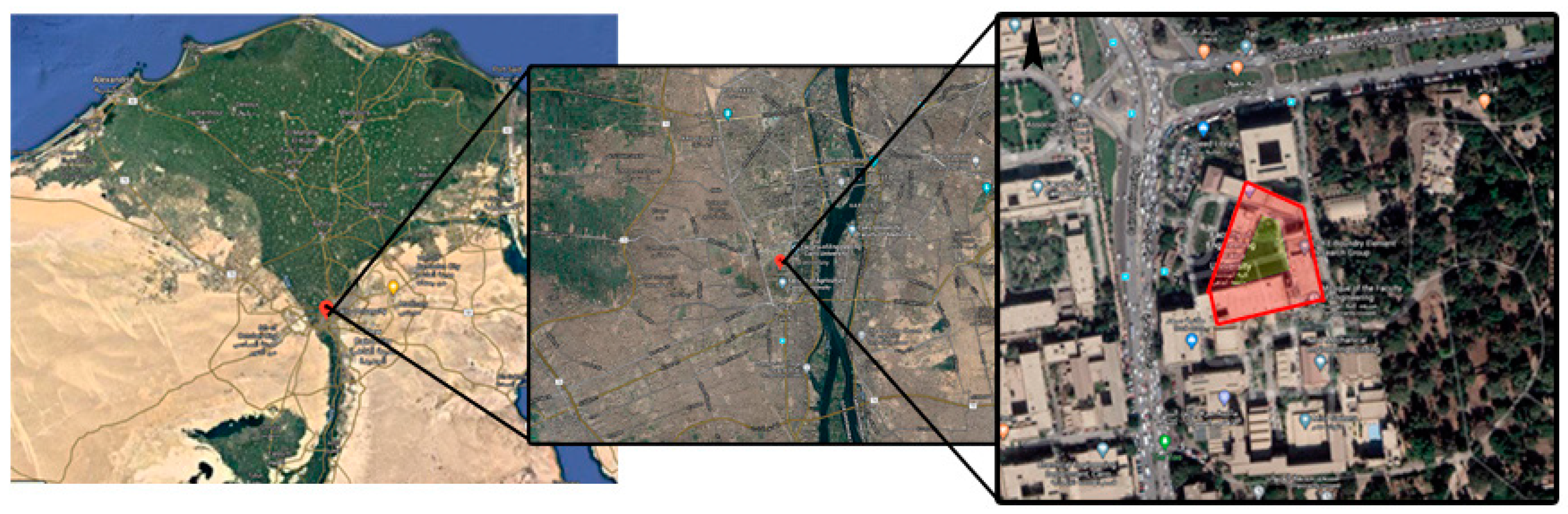
Figure 1 indicates the research case study location, architecture engineering department plaza of Cairo University, Giza, Egypt, which is located at 30.0131° N, 31.2089° E. Giza has a hot, arid climate and falls in the “hot desert climate” type according to the Köppen climate classification [25]. Giza receives a significant amount of solar radiation throughout the year. The average hourly maximum solar radiation exceeds 6 kWh/m2/d for almost 50% of the year [26].
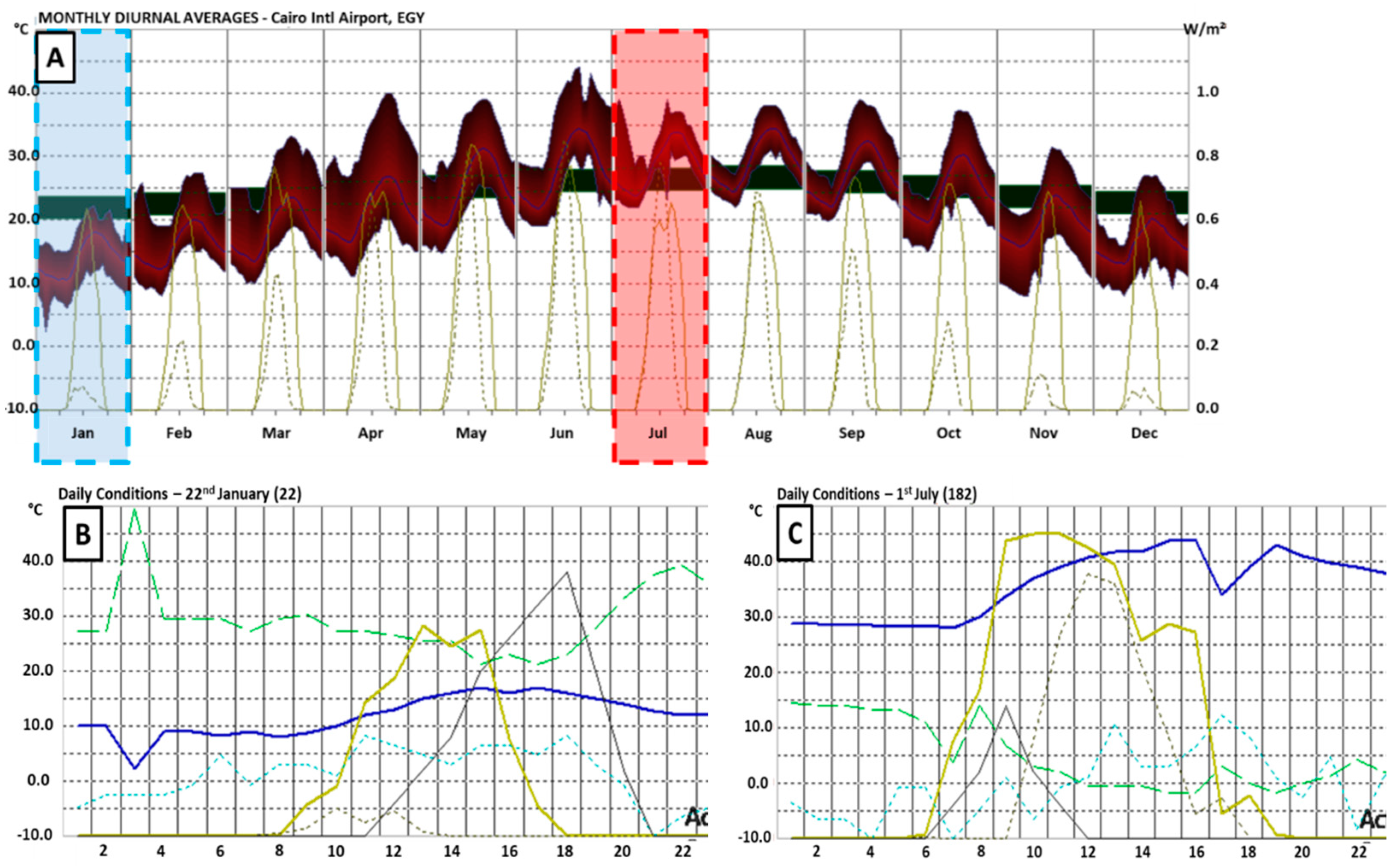
Ecotect weather analysis program was used to identify the two days that had the average temperature of each of the two seasons. Figure 2 Ecotect shows that the temperature on the 22nd of January matched the average temperature for the cold season and that on 1st July matched the average for the hot season.
1.1. Urban Geometry Characteristics
The grid of the eighteenth points Figure 3 comprises different urban geometry features and provides a variety of shading levels (e.g., under the trees’ crowns, near buildings, and in the un-shaded areas). Three sides of the semi-enclosed open space are surrounded by three streets (Table 1):
- Street 1 is a 6 m wide and WNW–ESE-oriented street. Four points were assigned in the middle of this street (1, 2, 3, and 4).
- Street 2 is a 6 m wide NNW–SSE oriented street from which four points were selected: three points (9, 10, and 14) near three trees—one near a large, old Cassia leptophylla tree and two near mature Cassia nodosa tree—and the last point (number 15) at the end of the street.
- Street 3 is a 6 m wide ENE–WSW-oriented street. Three points on it (16, 17, and 18) were selected.
- Zone 1 is a semi-enclosed open space, surrounded by the three streets mentioned above and one building, and two points (6 and 7) 1.5 m away from the building, to avoid long wave reflection and emission, were selected. Point (8) was directly under the canopy of a large old Cassia leptophylla tree. Five points (5, 8, 11, 12, and 13) were located in the middle of the open space in the sunny spots in the middle of the seating zone.
The finishing material of the seating area where seven points are located is yellow cement blocks, the albedo of which is 0.5, whereas the albedo of the asphalt of the surrounding streets is 0.2. Eleven points are located on these streets.
1.2. Vegetation Characteristics
Two types of the most common Egyptian urban environment trees are on the site. They are the deciduous/semi-deciduous C. nodosa and the semi-evergreen C. leptophylla. These trees’ physical characteristics, such as leaf area density (LAD) and the albedo values for each type at different heights, were adopted from [27]. Table 2 shows the simulation setup for the use of Leaf Area Index (LAI)-2000 (plant canopy analyzer instrument) [28].
2. Materials and Methods
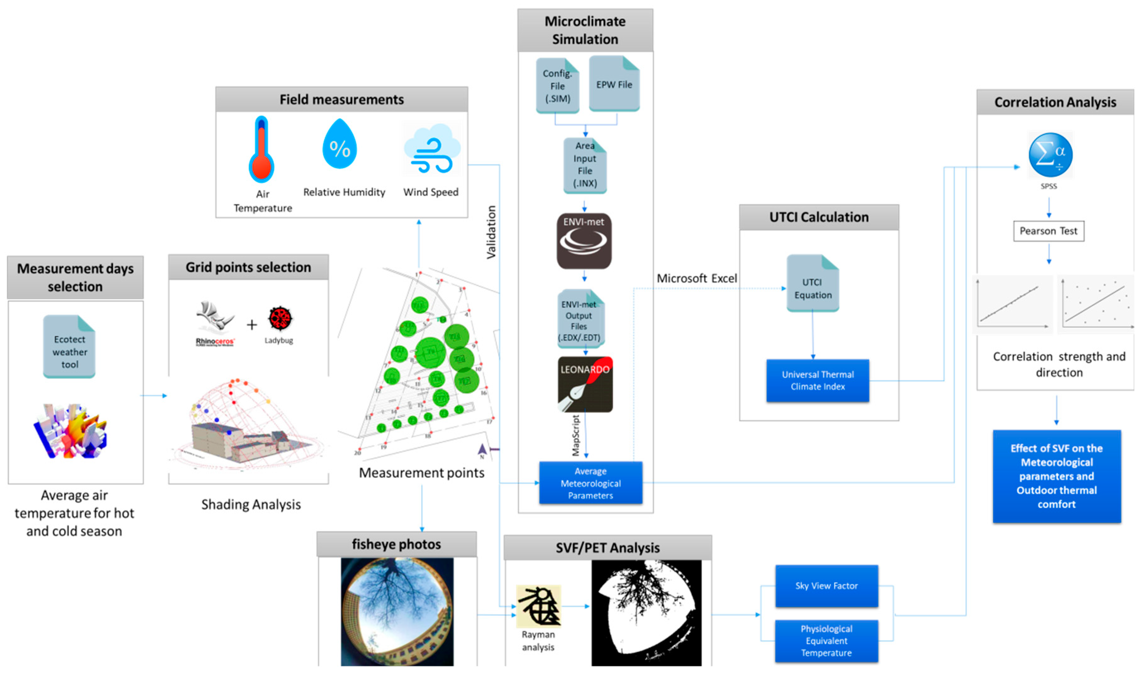
The study was structured in four stages: field measurements, numerical simulation, model validation, and statistical analysis (Figure 4). Two days with the average air temperature for both hot and cold seasons were selected for measurements and simulations based on weather analysis done using the Ecotect program [29].
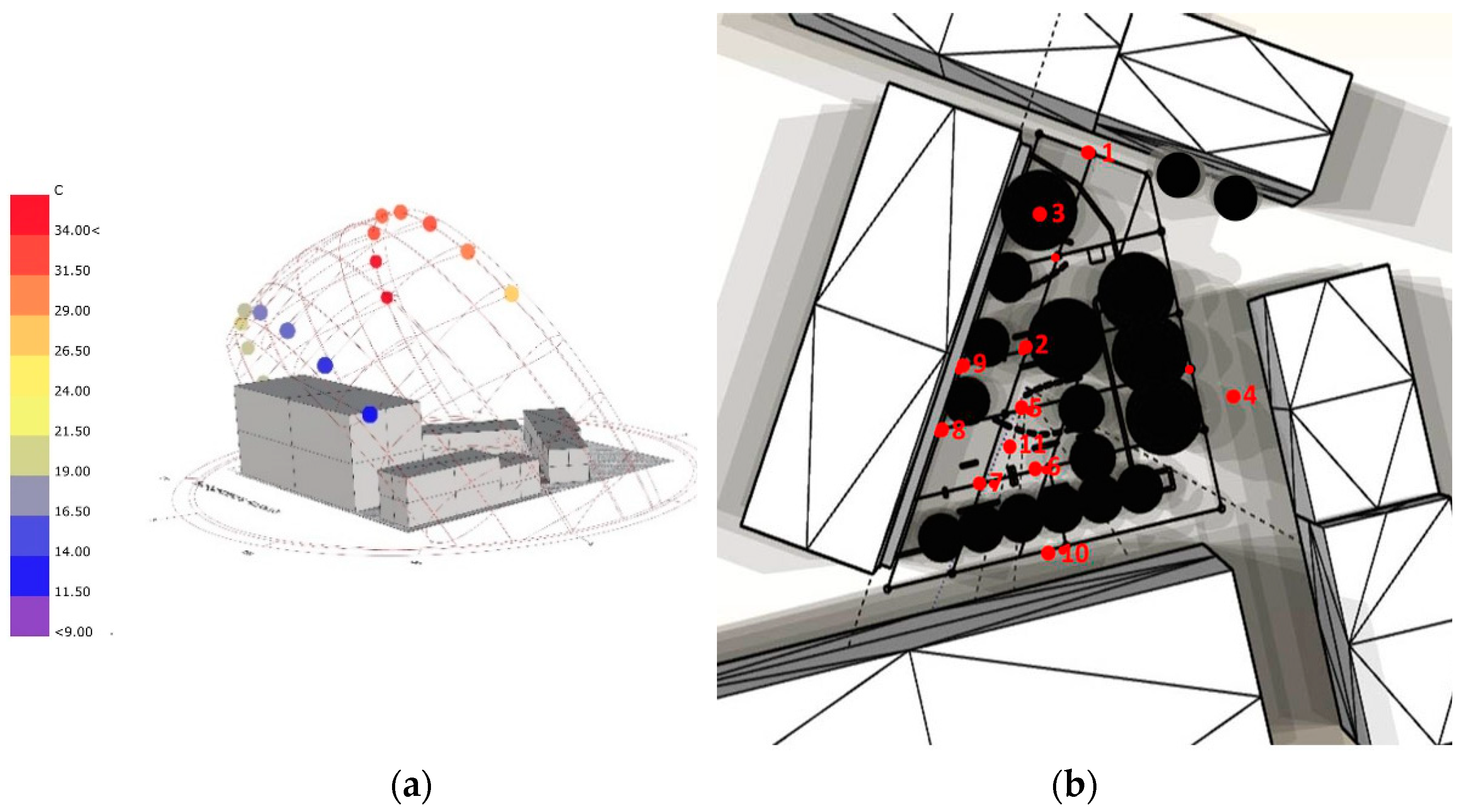
As shown in Figure 5a,b, shading analysis with sun path diagram identified 10 points for field measurements. According to the hours of occupation of the selected space from 09:00 to 17:00 according to the Local Solar Time (LST), ten points were selected and categorized into four types:
- Under the tree canopy,
- Center of the street canyon,
- Points exposed to solar radiation for more than 3 h,
- Points adjacent to buildings but at least 1.5 m away to avoid long waves radiated from buildings façades,
- Eight extra points in different locations were added to enlarge the sample size in the statistical analysis (Figure 3) for more reliable data.
2.1. Field Measurement
Field measurements were designed to verify model simulation through three steps:
- First: Measurement points were selected from shading analysis by detecting the points exposed to solar radiation for a long time using the Ladybug plug-in grasshopper.
- Second: Urban features in the open space were observed:
- ○
- Buildings numbers, orientation, height, and facades material.
- ○
- Landscape elements.
- ○
- Hardscape: The types of finishing materials, the area in m2, and artificial shading elements.
- ○
- Softscape: The number of trees, their location, types, and physical features.
- Third: For model validation, ten measurements were recorded, based on the number of occupation hours, for the microclimatic variables, namely, air temperature, relative humidity, and wind speed in the area. Portable Digital 5 IN 1Anemometer LM-8102 was used for the measurements Table 3.
2.2. SVF Analysis
SVF was calculated using photographic analysis:
- Hemispherical photos were taken using an external 180° fish-eye lens Table 3 connected to a 16-megapixel mobile camera at 1.5 height, looking up at the sky from each selected point for the measurement on both winter and summer days.
- The photos were uploaded to RayMan software for the analysis of the incidence of urban canyon geometry. The program analyzes the image turned into a high dynamic range (HDR) with the highest dynamic range of colors and shades and allowed, analyzing the pixel’s brightness value in question to arrive at the precise value of the analyzed SVF [31].
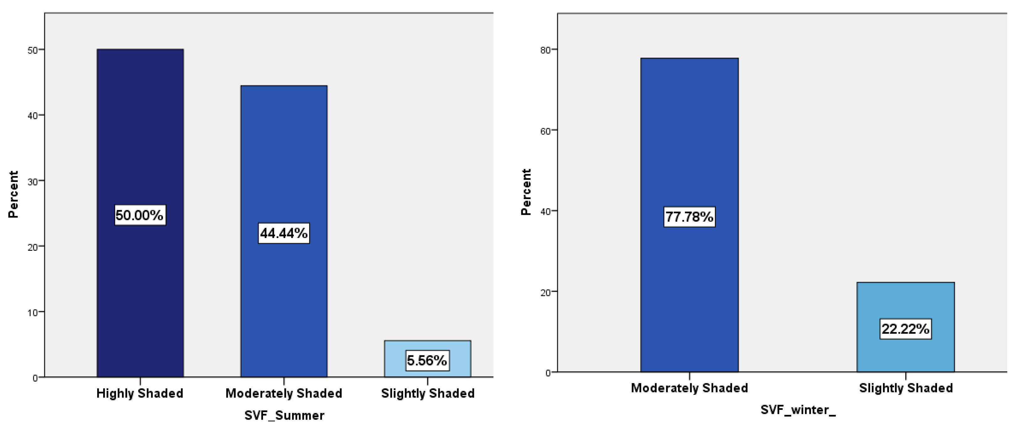
Table 4 shows the results of SVF values from the RayMan simulation. The SVF was classified into three shading levels following [32]: highly shaded areas (SVF < 0.3), moderately shaded areas (0.3 < SVF < 0.5), and slightly shaded areas (SVF > 0.5). As shown in Figure 6, during summer, 50% of the studied points were highly shaded, 44% were moderately shaded, and only 5% were slightly shaded, whereas SVF values in the street at points 1, 2, and Zone 1 were mostly moderately shaded and point 3 on street 3 was almost highly shaded. During winter, 77% of the studied points were moderately shaded, 22% were slightly shaded, and none of the points was highly shaded, which means that most of the site had moderately shaded areas. Generally, much of the site is moderately and highly shaded in both seasons.
In the hot season, the mean value of SVF was 0.29, and the minimum value was 0.05 in zone 1 at point 7, which was located between the two mature C. nodosa trees, whereas the maximum value of SVF was 0.49 in zone 1 at point 13 where the seating zone is located at an unshaded sunny spot. During the cold season, the mean SVF value was 0.45, and the minimum value of 0.33 was in zone 1 at point 18, and the maximum value of SVF, 0.60, was at point 4.
2.3. Numerical Simulation
The ENVI-met V4.0 software established numerical simulation. It is a 3D Computational Fluid Dynamics CFD numerical simulation tool that gathers the heat transfer mathematical models of soil–plant–building–air. Its data entered include the site meteorological parameters at the model boundary, urban and building geometries and materials’ physics, plant physiological, and photosynthesis parameters [33]. In contrast, its output data include SVF, Tmrt, all model grids, radiation environment, meteorology, and supports calculation of PET and Universal Thermal Comfort Index (UTCI), which are the scope of this research. ENVI-met has been used in many microclimatic urban analyses and has been validated by various studies [34,35], and its workflow includes four steps:
- Build a 3D model of the open space on ENVI-met by entering the following inputs: initial weather data, buildings geometry, soil type, and vegetation characteristics.
- Simulate the open space in both winter and summer to extract microclimatic variables, namely air temperature, relative humidity, mean radiant temperature, and wind speed at each hour to be used to calculate UTCI values [36].
- Extract meteorological data for the eighteen points at each hour.
The simulation was established for 22nd January 2018, the selected day in winter, and 1st July 2018, in summer. Input data was calibrated using the measured data. The boundary conditions and initial settings are presented in Table 5. A simple force condition was applied using hourly data from the EnergyPlus Weather (EPW) data file of Cairo International Airport. The wind speed input of 10 m was obtained from wind speed at the ground level by converting the formula from [37].
2.4. Model Calibration and Validation
Model simulation results of air temperature (Ta) and relative humidity (RH) were compared with the field measurements through correlation analysis by SPSS software [14]. R2 in the analysis described the strength of the relation between two variables.
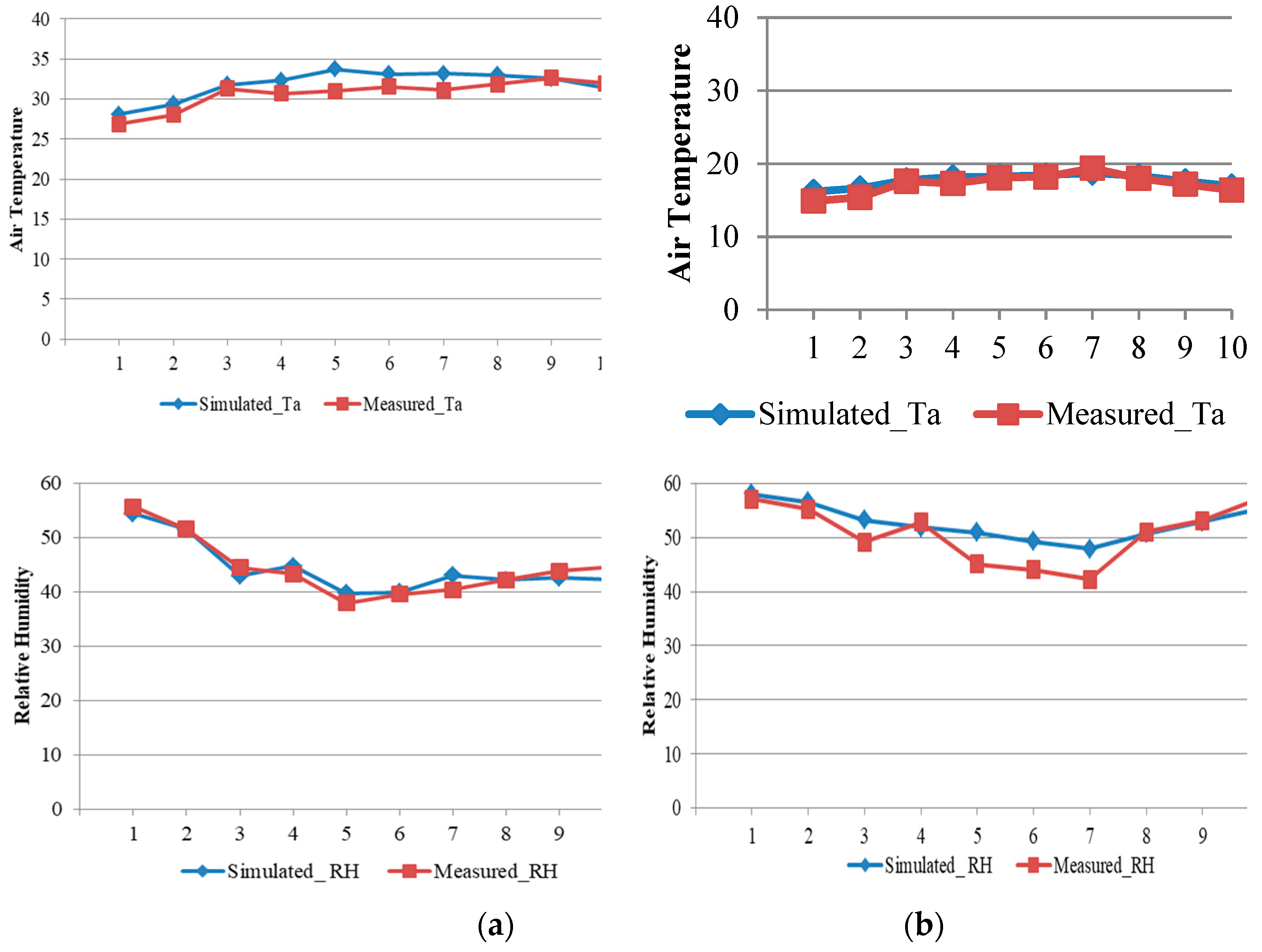
Figure 7 presents the relationship between the simulated and measured values, and Table 6 summarizes the validation of the model performance. It was found that there is a moderate correlation between the model and the measured data for Ta (r = 0.85) in summer, while it is much stronger in winter (r = 0.96). On the contrary, modeled RH showed a strong correlation of the model data with the measured data in summer (r = 0.95) and winter (r = 0.88). Therefore, ENVI-met simulation results in this study have an acceptable level of accuracy [38,39].
Various studies have calculated Tmrt relying on ENVI-met simulation [40,41], and others also showed that the simulated Tmrt had an overall agreement with their in situ measurements [42]. Therefore, in this study, Tmrt results were extracted from ENVI-met simulation. Different urban microclimate researchers compared wind speed in-field measurements with the simulation software to demonstrate the effectiveness and accuracy [10,43].
3. Results
Microclimatic variables were analyzed for eight hours from 09:00 to 17:00 while the selected space was occupied. The minimum value of air temperature was at point 17 at 09:00 LST in the hot season, and the mean radiant temperature was at its minimum at point 4 at 17:00 LST. The air temperature was at its maximum at point 11 at 13:00 LST, and the mean radiant temperature was at its maximum at point 8 at 14:00 LST. On the other hand, the minimum relative humidity was at point 11 at 13:00 LST, and the maximum was at 09:00 LST at point 13. The highest wind speed was recorded at point 18 at 17:00 LST, whereas the lowest wind speed was recorded at point 6 at 09:00LST. For each Ta, Tmrt, RH, and V, the values ranged between 28.85 and 34.1 °C, 30.83 and 75.4 °C, 37.2% and 53.1%, and 0.18 and 2.6 m/s, respectively.
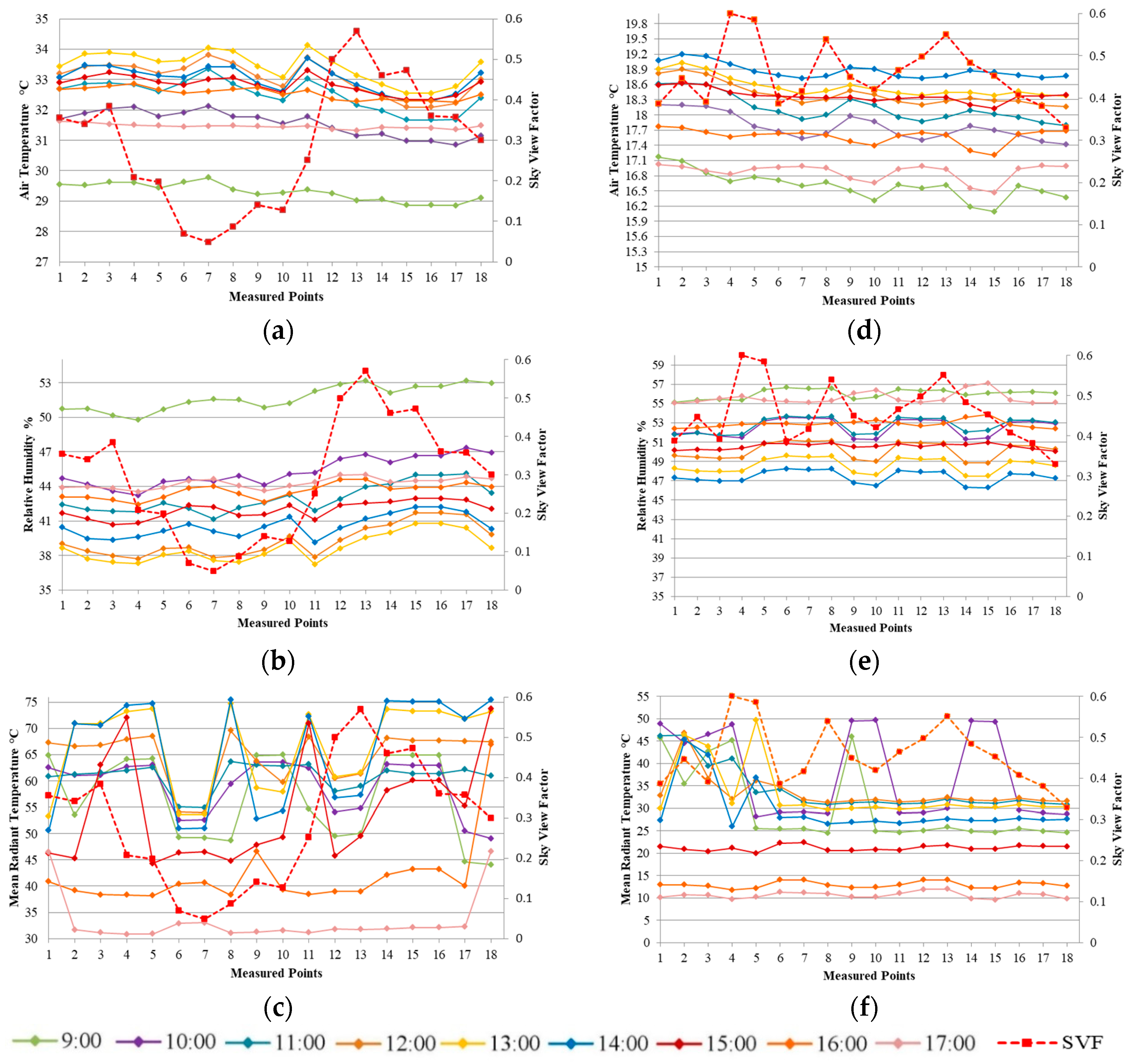
As shown in Figure 8a, throughout the simulation hours, the air temperature was increasing at all the 18 points before it declined noticeably after 13:00 LST, and they became roughly convergent at 17:00 LST. From 09:00 to 12:00 LST, Ta was the highest at point 7. However, from 13:00 to 15:00 LST, the air temperature at point 11 remained the highest and higher by 1 °C than at point 13, where the highest SVF was found. The lowest values were revealed in street 3, where values were lower by 0.1–1.3 °C than points in street 1—however, the temperature increased as they approached point 18. Moving from point 4 towards point 15, the Ta values decreased gradually toward the south–east along street 2. Overall, at most hours, peaks were observed at point 11 followed by point 7 and the points in street 1, while the minimum levels were observed in street 3.
In contrast with the Ta values, the highest values of RH (Figure 8b) for all points were at 09:00 LST and decreased at all the points before increasing at 13:00 LST, except at Point 11, which remained at the lowest values from 11:00 to 15:00 LST before it increased after 15:00 LST. The RH values at the points on street 3 were higher than at the points on street 1. However, they decreased towards point 18. In general, in the simulation, the difference between relative values for all points diminished as 17:00 LST approached.
In the simulation, the mean radiant temperature values at all hours and all points fluctuated as shown in Figure 8c, whereas from 09:00 to 14:00 LST, values at points 6, 7, and 8 were at their lowest values in comparison with the other points before they rose higher than others starting from 15:00 LST. Particularly at point 18, the Tmrt was higher by 18 °C than at point 17. At point 8, where SVF was low at 0.08, the Tmrt was nearly equal to the Tmrt at points 6 and 7 at 09:00 LST. After that, the Tmrt at point 8 increased and peaked at 14:00 LST, when it was higher than at points 6 and 7 by 24 °C. Thereafter, it decreased steeply by 30 °C to a level lower than at points 6 and 7. Like the Tmrt values at point 8, Tmrt at point 11 began rising and exceeded Tmrt at other points and peaked at 15:00 LST to exceed that at points 6 and 7 by 22 °C, a level of excess just less than that reached by the Tmrt at point 8. Thereafter, it decreased noticeably to become lower than the Tmrt at points 6 and 7. At point 8, it was lower by 31 °C than at point 13, where the highest average values of SVF and Tmrt were observed throughout the simulation. They reached their peak, 61.5 °C, at 13:00 LST. However, it was low in comparison with the values in street 1 and street 3. Generally, peaks at most of the hours were detected in streets 1 and 3, while minimum values were observed at the shaded points 6 and 7 in zone.
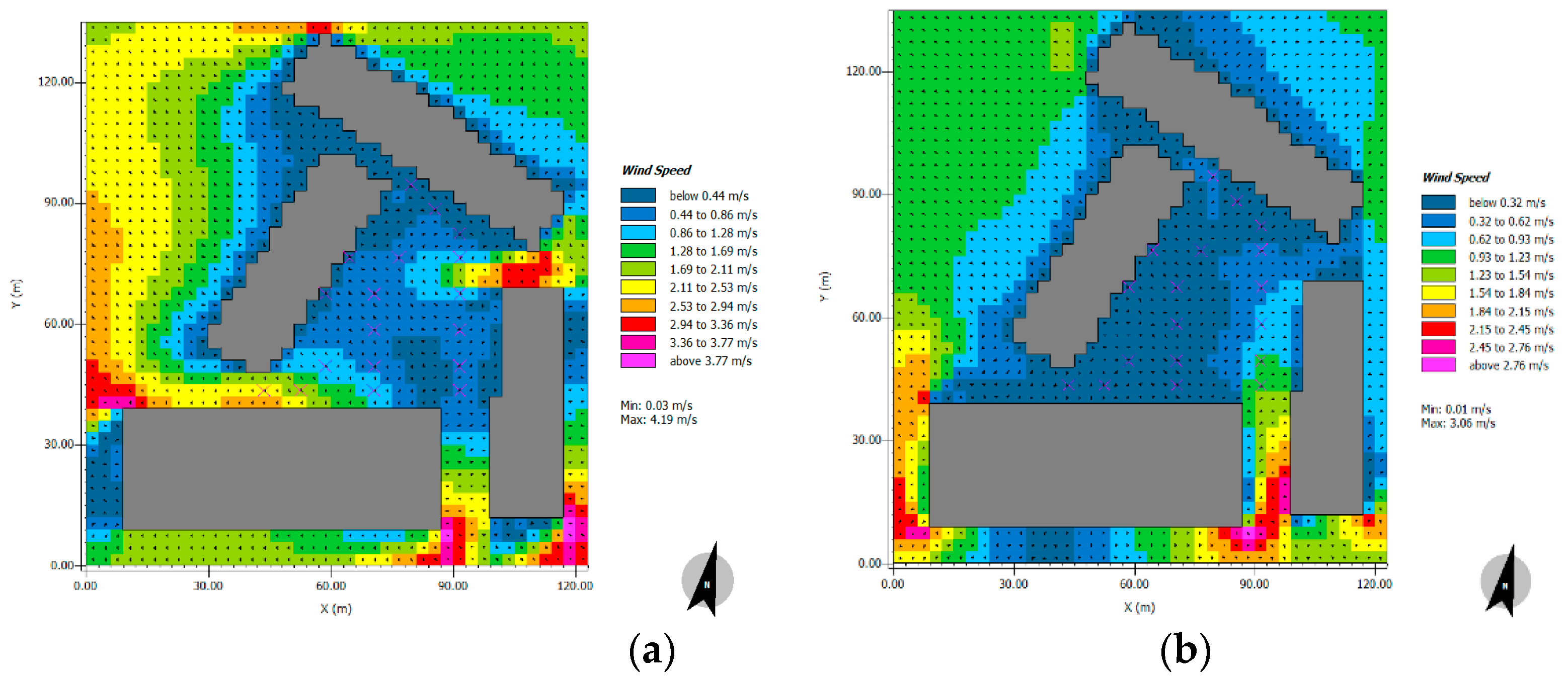
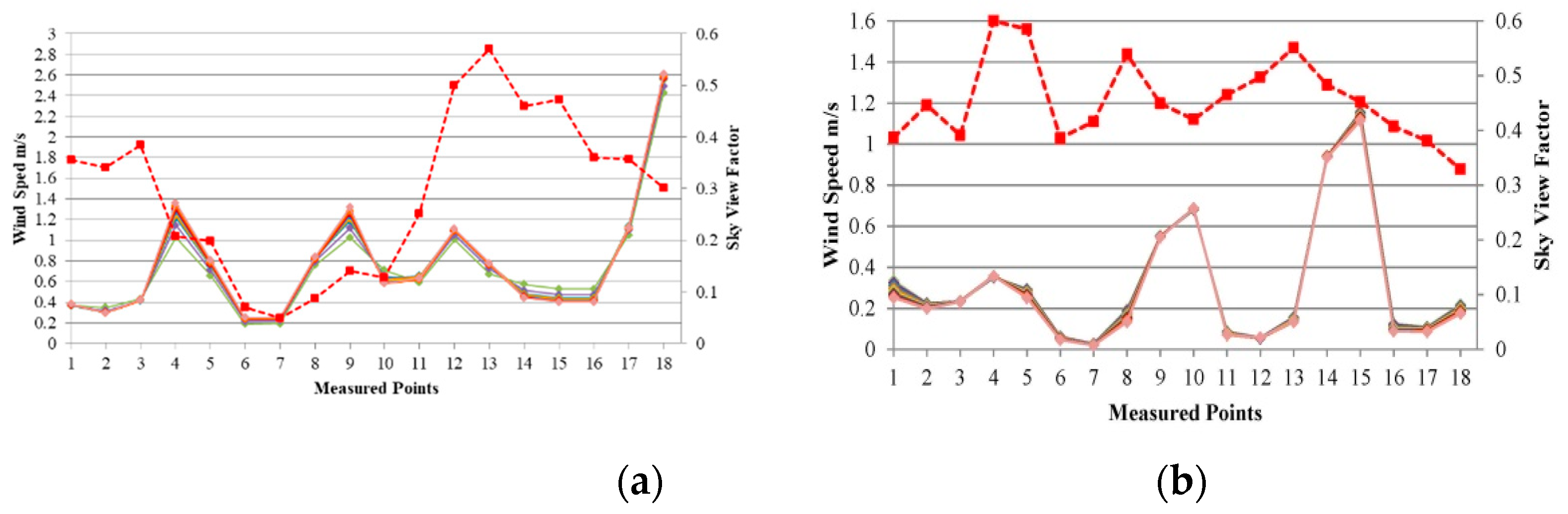
The prevailing wind direction was northeasterly Figure 9a. Wind speed in Figure 10a was almost steady at 0.18–2.6 m/s during all hours and at all points in the simulation. The values had an ascending trend from point 1 to point 4. It was lower at points in zone 1, particularly at points 6 and 7, where the lowest values were observed at 09:00 LST. The speed increased towards point 9. However, it decreased as one headed toward the south. On the contrary, the highest values were found in street 3, where it increased from point 16 and peaked at point 18. At the points in the middle of zone 1, such as points 5, 8, 11, and 12, the average values of V were higher by 0.4 to 0.6 m/s than at the points close to the building, such as points 6 and 7; however, V showed an ascending trend toward the south from point 5 toward point 12, where the V values were high throughout all hours in the simulation. In general, the lowest values were at points in street 1 as compared to street 2, while, in contrast, the highest values were at points in street 3.
In the cold season, the air temperature values ranged between 16.00 and 19.2 °C. As shown in Figure 8e, air temperature values at points in street 1 increased noticeably from 09:00 to 14:00 LST throughout all the simulated hours, and the highest value was observed at point 2 at 14:00 LST. At this hour, Ta was 18.9 °C at points 9 and 10 in street 2. These were among the highest values after point 2, while the lowest value was found at point 15 at 09:00 LST, followed by point 14. However, their Ta increased by 2.4 °C at 14:00 LST. Ta at points 6, 7, and 8 also increased as afternoon approached. However, the increase was between 0.1 and 0.4 °C, which was a lesser rate than that at the points in streets 1 and 2. Street 3’s values were among the lowest as compared to those in streets 1 and 2. A noticeable decrease of 0.7 °C at points 14 and 15 occurred at 15:00 LST. Generally, in all the simulation hours, the highest temperature values were recorded in street 1, whereas the lowest values were recorded in street 3.
The relative humidity values in Figure 8f ranged between 46.2% and 57.1%, and the highest values were at 09:00 LST and 17:00 LST, while the lowest values were at 14:00 LST with a reduction between 0.5% and 1.39% during the simulation. Both minimum and maximum values were recorded at point 15 followed by point 14 at 14:00 and 17:00 LST, respectively. Points in zone 1 and street 3 had a difference of 1%–2% higher than other points from 10:00 to 13:00 LST. A noticeable increment of 6% was at points in street 2 from 15:00 till 17:00 LST. Overall, at almost all simulation hours, the highest RH values were at points in zone 1 and street 3 compared to street 1 and street 2.
The mean radiant temperature in Figure 8g ranged between 9.06 and 49.60 °C, since the lowest Tmrt was at p15 at 17:00 LST while the highest value was at p5 at 13:00 LST. Points in street 1 showed high values of Tmrt in the forenoon, particularly at point 2, where values were high until 14:00 LST, when it noticeably decreased by 24.4 °C. Points in zone 1 remained roughly increasing by 2–4 °C until 13:00 LST, and then it began decreasing, except for point 5, where the highest value was revealed by an obvious increase of 13 °C from 12:00 LST to 13:00 LST before it decreased 12.8 °C at 14:00 LST. Point 10, point 14, and point 15 showed a noticeable increase of 25 °C from 09:00 to 10:00 LST; point 9 Tmrt was high at 09:00 and 10:00 LST, then it lowered to 18 °C at 11:00 LST. In general, values at points in street 1 were high in comparison to street 3 and zone 1 until 14:00 LST, followed by points 9 and 10 at street 2, which were high until 11:00 LST, relative to the other points.
As expected, the prevailing wind direction was blocked by surrounding buildings, reducing the release of trapped heat and RH. As shown in Figure 9, the prevailing wind direction was northwest, and wind speed in Figure 10b was unvaried through all the simulation hours at each point and ranged between 0.01 and 1.15 m/s. The highest values were found at point 15, followed by point 14, where V was 0.9 m/s, followed by point 10, where V was 0.6 m/s, and further followed by point 9, where V was 0.5 m/s. The lowest values were found at zone 1 at point 7 and point 6, followed by point 12 and point 11, where V was 0.05 and 0.08 m/s, respectively. Points in street 3 also demonstrated low values of V; however, their values were slightly higher before the afternoon. Moreover, V was higher by 0.1 m/s at point 18. Overall, all the highest values of V were observed in street 2 at point 15 and decreased as one moved northward. These were followed by values at points in street 1. The lowest values were in zone 1, particularly at points nearer to the 12 m high administrative building, such as at point 12, and it decreased gradually from points in the south, such as point 13, where V was 0.15 m/s, towards points located in the north until it was lowest at point 7 followed by point 6. Additionally, values at points in street 3, particularly at point 18, were higher than points in zone 1.
3.1. SVF, Microclimatic Variables and Thermal Comfort
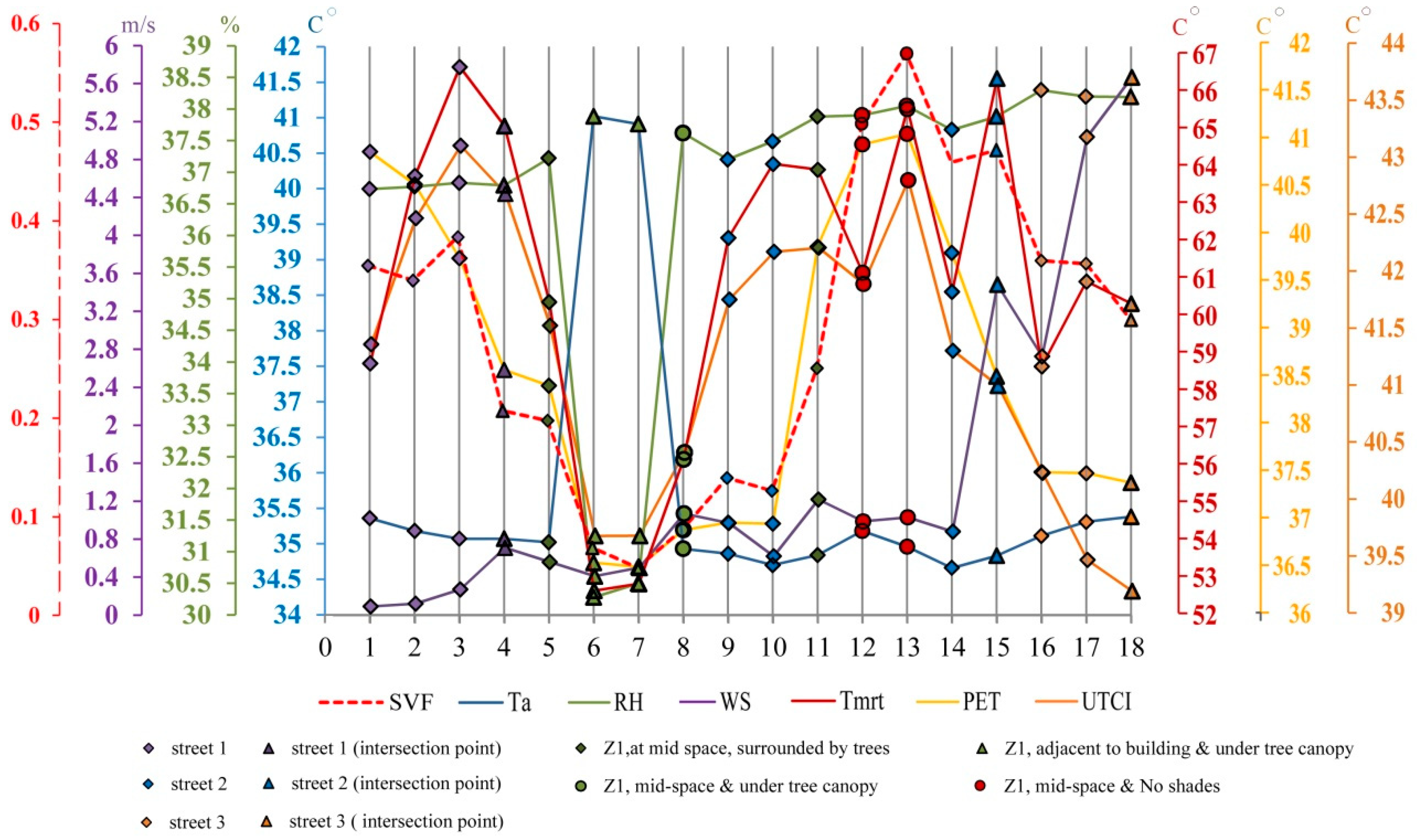
As shown in Figure 11 and Figure 12, the 18 points were categorized according to their location in the open space, describing the surrounding urban features from Table 1. In the summer (Figure 11), SVF ranged from 0.04 to 0.5, and the average air temperature Ta_avg ranged from 31.6 to 32.6 °C. The highest value was found at point 7 despite the lowest SVF value of 0.049 that it had. They were followed by point 11, where the Ta_avg was 32.6 °C. Points in street 1 showed high values of Ta_avg between 32.3 and 32.5 °C compared to street 3, where the lowest value, 31.6 °C, was found. However, there was a slight increase of 0.5 °C at point 18. Ta_avg values were 32.3 °C at point 5 and point 6 increased by 0.1 °C at point 8. The highest SVF value was observed at point 13, followed by point 12; these points showed low values of Ta_avg at 31.9 °C and 32.1 °C, respectively.
The average relative humidity, RH_avg, highest values were found at the points in street 3 since the highest value was 44.6% at point 17 followed by point 16 and point 15, while it decreased 1% at point 18. The lowest values were found at street 1 at point 4, where RH_avg was 41.8%, and it increased gradually towards point 1 where the value was 42.7%. A slight difference of 0.1% was observed among points located in zone 1 where values were between 42.4% and 42.9%; a slight rise of 1.5% at point 12 and point 13 was also observed. In street 2, values continued to increase, starting from point 9 (42.5%) towards point 14 (43.95%).
Concerning Tmrt, the highest average value was 62 °C observed at point 18 despite its location in the deep canyon. Moreover, it had the highest value of an average wind speed of 2.5 m/s. On the other hand, it was found that the lowest value of Tmrt_avg was 48.4 °C at point 6, which also demonstrated the lowest value of wind speed, 0.2 m/s. At points in street 1, these values increased towards point 4 to reach 60.6 °C and 1.2 m/s with a difference of 6 °C and 0.9 m/s from point 1, respectively.
In terms of outdoor thermal comfort indices, PET average values ranged from 36.8 to 41.07 °C, while UTCI ranged from 28.4 to 31.6 °C. PET and UTCI showed their lowest average values at both points 7 and 6, which were 36.8 °C and 28.4 °C, respectively, whereas the lowest values of SVF were also seen. The highest value of PET_avg was at point 13, followed by point 12, where the highest values of SVF also was recorded, while the highest value of UTCI_avg was 31.62 °C at point 4. All points were considered to be uncomfortable for PET values since the thermal comfort ranged 23–32 °C [44]. Meanwhile, regarding UTCI values, according to the UTCI assessment scale [36], all points indicated moderate heat stress, even the lowest values.
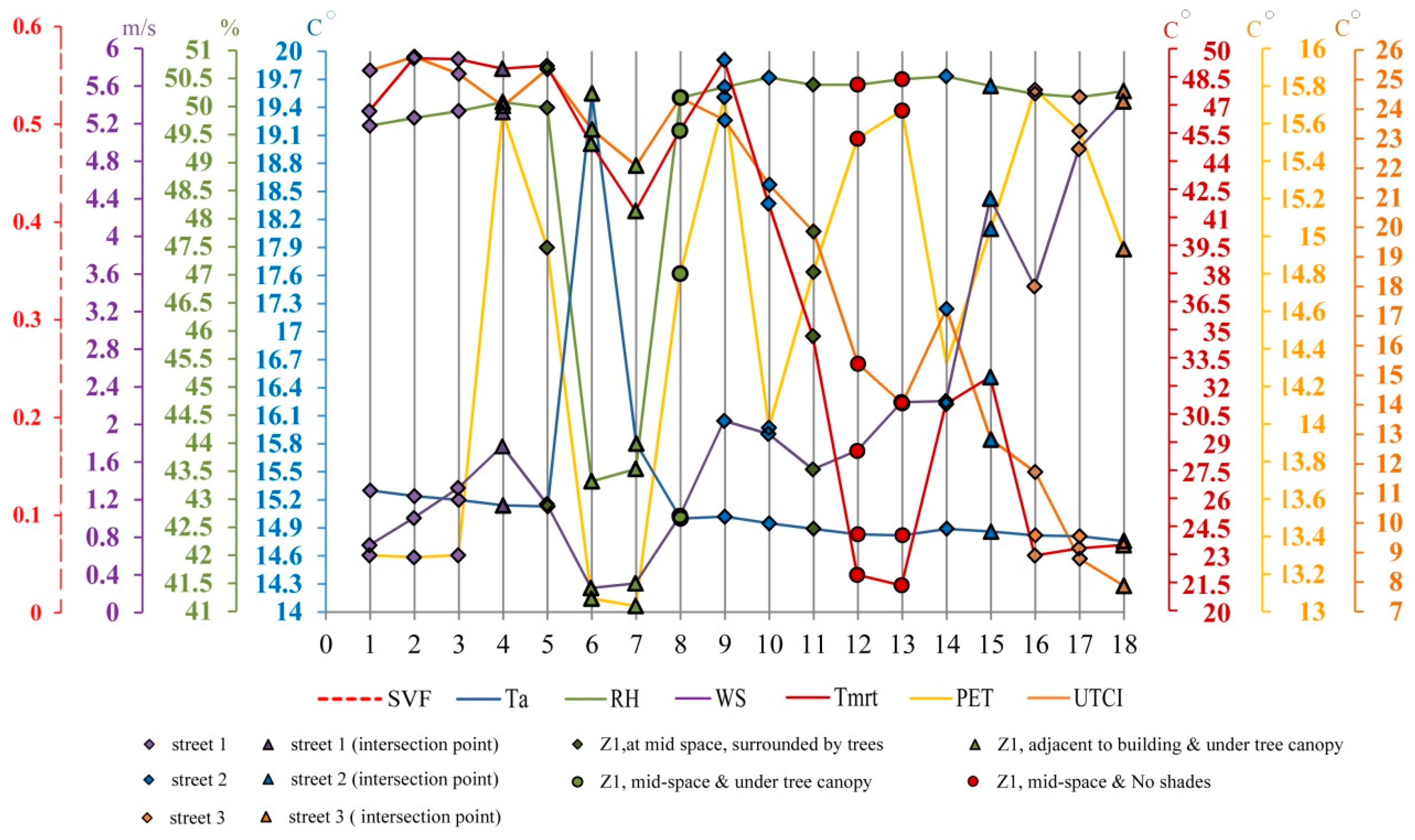
In the cold season, SVF values ranged 0.3–0.6 and Ta_avg ranged from 17.6 to 18.2 °C (Figure 12). Point 2, with an SVF of 0.4, showed the highest value of Ta_avg and Tmrt_avg and UTCI, which were 34.3 and −0.35 °C, respectively. The lowest value of Ta_avg was demonstrated at point 15, accompanied by the highest value of V_avg 1.1 m/s. Ta_avg values in street 1 were the highest in comparison to street 2 and 3. Ta_avg under tree canopy in zone 1 at point 8 was 17.8 °C, where the lowest value of Tmrt_avg was 24 °C. On the other hand, the minimum value of RH_avg was 51.2% at point 3 with SVF = 0.39; the maximum value was 52.4% at point 6, where SVF equals 0.3. Point 7 showed the lowest V_avg 0.02 m/s as it showed the lowest value of PET_avg 13 °C. The highest value of PET was 15.78 °C found at point 16, although Ta_avg was 17.8 °C. The lowest value of the UTCI value was −4.4 °C at point 18, where the lowest SVF value, 0.32, was found.
3.2. Correlation between SVF, Microclimatic Variables, and Thermal Comfort
Finally, at the statistical analysis phase, the correlation between SVF and the average values of the microclimatic variables, PET and UTCI, which are required to express the central tendency of the results during the whole period of occupation at each point, was analyzed throughout the daytime during both seasons, with the average values of each variable indicated by Ta_avg, Tmrt_avg, RH_avg, V_avg, PET_avg, and UTCI_avg.
Table 7 shows Pearson’s bivariate test (r) to explore the strength and type of correlation between variables considering the significance level and r coefficient interpretation, since there is no correlation when r = 0, it is weak when 0 < r < 0.25, it is moderate when 0.25 < r < 0.75, and it is strong when r > 0.75 [45]. In the summer, the test showed a moderate correlation between SVF and Ta, Tmrt, RH, PET, and UTCI as r = −0.57, r = 0.71, r = 0.51, r = 0.68, and r = 0.53, respectively. On the other hand, the correlation of V with SVF was not at a significant level. In the winter, SVF showed no correlation with any microclimatic variables, even PET and UTCI.
Table 8 illustrates the correlation between SVF and the microclimatic variables, PET and UTCI, which showed a correlated linear variation significantly in the Pearson test for the two seasons. Regarding SVF and Ta_avg Equation (1), the intercept a = 32.52 implies that Ta_avg at a completely shaded point with no sun penetration was 32.52 °C. Furthermore, the slope b = −1.15 expresses that Ta_avg decreased 0.1 °C per 0.1 unit increase in SVF, which indicates the lesser the shade at any point, the lesser will be the average air temperature.
At Tmrt_avg Equation (2), the slope b = 25.63 is equivalent to an increase in Tmrt_avg value by 2.5 °C per 0.1 unit of SVF, which indicates the lesser shade at any point, the more mean radiant temperature the occupants experience at this point. Tmrt at a completely shaded area equals 49.9 °C, while RH showed a positive correlation with SVF since it increased 0.3% per each 0.1 unit increase in SVF RH_avg Equation (3). Moreover, it equals 42.2% at a completely shaded point. In SVF and PET_avg Equation (4), intercept a = 36.3 °C (uncomfortable) determined that PET was 36.3 °C at a completely shaded point, and it increased 0.4 °C per 0.1 unit increase in SVF according to the slope (b = 7.92). UTCI_avg Equation (5) showed a lower value (28.61 °C) at the completely shaded point, and it increased by 2.5 °C at each 0.1 unit increase in SVF.
Ta_avg Equation (1)
y = 32.52 − 1.15 × x
Tmrt_avg Equation (2)
y = 49.95 + 25.63 × x
RH_avg Equation (3)
y = 42.22 + 3.17 × x
PET_avg Equation (4)
y = 36.3 + 7.92 × x
UTCI_avg Equation (5)
y = 28.61 + 5.87 × x
4. Discussion
This study investigated the relation between SVF, microclimatic variables, and outdoor thermal comfort in an open space in a hot and arid environment. Since the open space includes different landscape elements, the study applied a photographic method to extract SVF values and ENVI-met Simulation to extract microclimatic variables values in 18 points corresponding to different urban elements’ geometry. Studying urban microclimate of the architecture engineering department plaza of Cairo University is very different from street canyons, as campuses may include different, irregular urban spaces with different occupation time schedules due to their differentiated activities as a livable place rather than a passage. Regardless of the plaza’s small area having a high building density area, it is used by up to 80 students; sheltering them from excessive solar radiation is crucial.
Effect of Shading on Microclimatic Variables and Outdoor Thermal Comfort
Shading in the open space was provided at points shaded by trees or buildings or by both. Of the points, 33% were shaded by both trees and buildings, whilst 39% were shaded only by buildings on paved streets. Additionally, 28% were non-shaded and in the middle of the space. In the hot season in Table 7, SVF showed a negative correlation with average air temperature. Regarding shaded points by trees and building, this result can be interpreted as due to the shade of trees of smaller spread with low wind speed, which could negatively impact Ta because, without air flowing to transport the trees’ cooling effect (evapotranspiration) to the open spaces from the shaded areas [46,47], static hot air caused an increase in air temperature under the trees’ canopy. Additionally, the longwave radiation is emitted not only by the ground but also by tree leaves [48]. The longwave radiation was greater in shaded areas than in open ones, which could have contributed to the higher air temperature under the tree canopy, particularly as high average LAD was found at point 7 under the C. nodosa tree, which is close to the 12 m high building with the minimum SVF and the lowest wind speed, Ta was higher by 0.1 °C than that at point 13, which was non-shaded in the middle of zone 1 and with the maximum value of SVF. For the previously mentioned reasons, contrary to point 7, Ta and RH at point 8, where C. leptophylla tree was, were lower by 0.1 °C and 0.2%, while V was higher by 0.5 m/s; this result agrees with [21], who found that wind speed was more related to the tree trunk height than tree foliage, as the higher the trunk was, the higher the wind speed was. Concerning air temperature increment at points located on the pavement under C. nodosa’s shade, such as point 4 in street 1, it was found that Ta was lower than at point 7 by 0.1 °C because of V, which was higher by 1 m/s than at point 7 due to the location of point 4 at the intersection of two streets. In comparison, points 9 and 10 in street 2 under C. leptophylla tree showed a lower value of 0.3–0.5 °C because of street orientation, higher wind speed, and a taller tree trunk. Points located in the surrounded streets that were not under tree cover, such as point 2, had a high Ta due to the high absorptive ability of the dark color of asphalt. It absorbs great amounts of solar radiation and re-emits the absorbed radiation to the surrounded bodies [49]. However, street orientation coupled with H/W has a noticeable impact on air temperature because Ta at points in street 3 were lower by 0.5 °C than those in street 1. Moreover, Ta at point 15 was the lowest since it was located at high H/W.
Relative humidity correlated positively with SVF since it was much higher in non-shaded areas than at the shaded points. RH was low under C. nodosa shade at point 7 because the high air temperature attenuated the evapotranspiration process. The highest values were in street 3 because of the low values of air temperature. In addition, there were six C. nodosa trees on one side of the street raised the effect of the evapotranspiration process.
On the other hand, SVF showed a direct correlation with Tmrt and had a significant effect on it. This result agrees with [13,36,50]. The difference in the mean radiant temperature at all points changed over time depending on the Sun’s position, whereas Tmrt was at its highest value at point 13 due to its location farther away from the obstacles, so it received the most extensive solar radiation. It was followed by point 11. Altitude angles of the Sun at 11:00, 12:00, 14:00, and 15:00 LST were 61° and 73° from the east before midday and from the west after midday, and azimuth angles were 101°, 120°, 237°, and 257°, respectively, as it is noticed that altitude angles are nearest to the perpendicular angle above point 11, which makes it most exposed to more direct solar radiation. Additionally, the Tmrt value at point 7 was less than at point 8, though both are located under trees. The trees are of different species and physical parameters, which cause a different impact on Tmrt. In addition, the spatial location of point 7 was closer to the 12 m high building, which blocked solar radiation at some hours [50].
Wind speed rose along all points located in street 3 and peaked at point 18 because wind speed increased due to the funneling effect that the canyon has on the wind with the different orientation of streets and buildings, causing greater wind turbulence [13,51]. Wind speed varied with the orientation of streets since the lower values were registered in street 1 while the maximum values were observed in street 3. In street 2, we observed that values increased northward. These results can be attributed to the prevailing wind turbulence caused by the various building orientations as indicated by the fact that points located at a street intersection, such as points 4, 15, and 18, showed high wind speed values.
PET and UTCI showed a correlation with SVF that agrees with [13,52], which showed that SVF has a significant effect on PET. Despite the greater percentage of shaded areas in the case study, it was uncomfortable during the summer according to the PET index and caused moderate heat stress in terms of the UTCI Index.
In the winter, Tmrt was more related to the effect of urban geometry and according to the Sun’s path because the trees in the open space are deciduous, which made for the high SVF values at points that were shaded by the trees in summer. Therefore, the 32 m building in the south of the open space coupled with a low solar altitude had the effect of blocking the direct solar radiation from points in street 3 and zone 1, and they had correspondingly low values of Tmrt throughout the simulation hours. On the contrary, Tmrt fluctuated noticeably at points in street 1, where the highest average value was at point 2 before 14:00 LST, when the difference caused by the decrease—points 9 and 10 in street 2—also reached 30 °C.
In winter, when the plaza is not under the same heat stress of summer, occupant and pedestrian thermal comfort relied more on the buildings that provided shade at low solar altitude and less solar radiation; at the same time, trees discarded their leaves. In contrast, the plaza faced a high solar altitude and radiation in summer and trapped heat and blocked prevailing wind by the northwest building, which is why trees did not provide more significant improvements in Tmrt values. From these standing points, thermal comfort’s correlation with SVF is variant, and it is better to correlate only Tmrt to SVF because SVF controls short-wave and, to some extent, longwave radiation efficiently, more than all other meteorological factors that affect thermal comfort. It can be suggested to provide either solar shelter by light shading devices at the excessive heat stress un-shaded points (but trapping heat might increase) or plant a ground grass coverage to reduce the ground latent heat and provide evapotranspiration effect without trapping heat by trees. However, the strong correlation between SVF and Tmrt suggests that for new universities’ campuses, both buildings’ and trees’ land uses must be investigated in correlation to Tmrt.
5. Conclusions
In this study, the impact of SVF on microclimatic variables and outdoor thermal comfort conditions have been investigated using ENVI-met simulation summer and winter on a university campus at Giza, Egypt, to study the effect of urban geometry on the thermal performance at different points in an open space and to support the existing body of knowledge in thermal comfort studies in Egypt.
For further enhancement of the thermal comfort condition in outdoor spaces in the hot arid region of Egypt, the study draws attention to the following points:
- In summer, SVF affected microclimatic variables and outdoor thermal comfort. However, SVF’s effect on Tmrt and PET was more significant than on Ta, RH, and UTCI.
- SVF showed a negative effect on air temperature, whereas average air temperature was higher at points under some trees’ shade. This implied that excessive shade at points located on low-albedo materials, such as asphalt, particularly when wind speed is low, could negatively impact air temperature. However, the air temperature was not a significant indicator of thermal comfort; rather, the mean radiant temperature was consistent with both PET and UTCI.
- In contrast with the air temperature, SVF showed a positive correlation with mean radiant temperature, indicating that the lesser the shade, the higher Tmrt.
- The shades of different tree species differed according to their spatial location in relation to the surrounded buildings and their physical parameters. The air temperature was lower under trees with taller trunks and lower average LAD.
- Though SVF showed a positive but variant correlation with both PET and UTCI, it had a more significant effect on PET, and it is better to correlate SVF with Tmrt.
- This research’s main insight was the correlation between SVF and Tmrt, which emphasizes the importance of using urban trees to modify the radiation environment of already existing university campuses’ open spaces as shown in Table 7 and Table 8 and their related statistical significance analysis. These correlations are remarked upon for similar sites’ landscape sketch designs to suggest specific trees and plantation patterns to control SVF and generate a definite area of ground shading. However, over-shading by trees canopies must be considered as it might cause a reversed thermal effect, especially in existing sites that have prevailing wind blockage by surrounding buildings.
Author Contributions
Conceptualization, R.O.S., A.H.M. and M.F.; methodology, R.O.S., A.H.M. and M.F.; software, R.O.S.; validation, R.O.S.; formal analysis, R.O.S., A.H.M. and M.F.; investigation, R.O.S. and M.F.; resources, R.O.S., A.H.M. and M.F.; data curation, R.O.S., A.H.M. and M.F.; writing—original draft preparation, R.O.S., A.H.M. and M.F.; writing—review and editing, R.O.S., A.H.M. and M.F.; visualization, R.O.S., A.H.M. and M.F.; supervision, A.H.M. and M.F. All authors have read and agreed to the published version of the manuscript.
Funding
This research received no external funding.
Institutional Review Board Statement
Not applicable.
Informed Consent Statement
Not applicable.
Data Availability Statement
Data sharing not applicable.
Conflicts of Interest
The authors declare no conflict of interest.
Abbreviations
| SVF | Sky View Factor |
| H/W | Aspect ratio |
| LAI | Leaf Area Index |
| LAD | Leaf Area Density |
| Tmrt | Mean radiant temperature |
| Ta | Air temperature |
| RH | Relative Humidity |
| V | Wind Speed |
| PET | Physiological Equivalent Temperature |
| UTCI | Universal Thermal Comfort Index |
References
- Boukhelkhal, I.; Bourbia, P.F. Thermal Comfort Conditions in Outdoor Urban Spaces: Hot Dry Climate —Ghardaia—Algeria. Procedia Eng. 2016, 169, 207–215. [Google Scholar] [CrossRef]
- Nouri, A.S. A Framework of Thermal Sensitive Urban Design Benchmarks: Potentiating the Longevity of Auckland’s Public Realm. Buildings 2015, 5, 252–281. [Google Scholar] [CrossRef] [Green Version]
- Mirzaee, S.; Özgun, O.; Ruth, M.; Binita, K. Neighborhood-scale sky view factor variations with building density and height: A simulation approach and case study of Boston. Urban Clim. 2018, 26, 95–108. [Google Scholar] [CrossRef]
- Fahmy, M.; Mahmoud, S.; Elwy, I.; Mahmoud, H. A Review and Insights for Eleven Years of Urban Microclimate Research Towards a New Egyptian ERA of Low Carbon, Comfortable and Energy-Efficient Housing Typologies. Atmosphere 2020, 11, 236. [Google Scholar] [CrossRef] [Green Version]
- Bourbia, F.; Boucheriba, F. Impact of street design on urban microclimate for semi arid climate (Constantine). Renew. Energy 2010, 35, 343–347. [Google Scholar] [CrossRef]
- Lin, P.; Gou, Z.; Lau, S.S.Y.; Qin, H. The Impact of Urban Design Descriptors on Outdoor Thermal Environment: A Literature Review. Energies 2017, 10, 2151. [Google Scholar] [CrossRef] [Green Version]
- Lyu, T.; Buccolieri, R.; Gao, Z. A Numerical Study on the Correlation between Sky View Factor and Summer Microclimate of Local Climate Zones. Atmosphere 2019, 10, 438. [Google Scholar] [CrossRef] [Green Version]
- Fahmy, M.; Sharples, S. Passive design for urban thermal comfort: A comparison between different urban forms in Cairo, Egypt. In Proceedings of the PLEA 2008—25th Conference on Passive and Low Energy Architecture, Dublin, Ireland, 22–24 October 2008. [Google Scholar]
- Mahmoud, A.H.A. An analysis of bioclimatic zones and implications for design of outdoor built environments in Egypt. Build. Environ. 2011, 46, 605–620. [Google Scholar] [CrossRef]
- Krüger, E.L.; Minella, F.; Rasia, F. Impact of urban geometry on outdoor thermal comfort and air quality from field measurements in Curitiba, Brazil. Build. Environ. 2011, 46, 621–634. [Google Scholar] [CrossRef]
- Wang, Y.; Akbari, H. Effect of Sky View Factor on Outdoor Temperature and Comfort in Montreal. Environ. Eng. Sci. 2014, 31, 272–287. [Google Scholar] [CrossRef]
- Oke, T.R. Boundary Layer Climates; Methuen: London, UK, 1987. [Google Scholar]
- Venhari, A.A.; Tenpierik, M.J.; Taleghani, M. The role of sky view factor and urban street greenery in human thermal comfort and heat stress in a desert climate. J. Arid. Environ. 2019, 166, 68–76. [Google Scholar] [CrossRef]
- Baghaeipoor, G.; Nasrollahi, N. The Effect of Sky View Factor on Air temperature in High-rise Urban Residential Environments. J. Daylighting 2019, 6, 42–51. [Google Scholar] [CrossRef] [Green Version]
- Zhu, Z.; Liang, J.; Sun, C.; Han, Y. Summer Outdoor Thermal Comfort in Urban Commercial Pedestrian Streets in Severe Cold Regions of China. Sustainability 2020, 12, 1876. [Google Scholar] [CrossRef] [Green Version]
- Abaas, Z.R. Impact of development on Baghdad’s urban microclimate and human thermal comfort. Alex. Eng. J. 2020, 59, 275–290. [Google Scholar] [CrossRef]
- Lin, T.-P.; Matzarakis, A.; Hwang, R.-L. Shading effect on long-term outdoor thermal comfort. Build. Environ. 2010, 45, 213–221. [Google Scholar] [CrossRef]
- Xi, T.; Li, Q.; Mochida, A.; Meng, Q. Study on the outdoor thermal environment and thermal comfort around campus clusters in subtropical urban areas. Build. Environ. 2012, 52, 162–170. [Google Scholar] [CrossRef]
- Santamouris, M. Energy and Climate in the Urban Built Environment, 1st ed.; Routledge: London, UK, 2001. [Google Scholar]
- Abdallah, A.S.H.; Hussein, S.W.; Nayel, M. The impact of outdoor shading strategies on student thermal comfort in open spaces between education building. Sustain. Cities Soc. 2020, 58, 102124. [Google Scholar] [CrossRef]
- Morakinyo, T.E.; Ka-Lun, L.K.; Chao, R.; Ng, E. Performance of Hong Kong’s common trees species for outdoor temperature regulation, thermal comfort and energy saving. Build. Environ. 2018, 137, 157–170. [Google Scholar] [CrossRef]
- Mullaney, J.; Lucke, T.; Trueman, S.J. A review of benefits and challenges in growing street trees in paved urban environments. Landsc. Urban Plan. 2015, 134, 157–166. [Google Scholar] [CrossRef]
- Armson, D.; Stringer, P.; Ennos, A. The effect of tree shade and grass on surface and globe temperatures in an urban area. Urban For. Urban Green. 2012, 11, 245–255. [Google Scholar] [CrossRef]
- Fahmy, M.; Sharples, S.; Yahiya, M. LAI based trees selection for mid latitude urban developments: A microclimatic study in Cairo, Egypt. Build. Environ. 2010, 45, 345–357. [Google Scholar] [CrossRef] [Green Version]
- Kottek, M.; Grieser, J.; Beck, C.; Rudolf, B.; Rubel, F. World Map of the Köppen-Geiger climate classification updated. Meteorol. Z. 2006, 15, 259–263. [Google Scholar] [CrossRef]
- Diab, F.; Lan, H.; Zhang, L.; Ali, S. An Environmentally-Friendly Tourist Village in Egypt Based on a Hybrid Renewable Energy System––Part One: What Is the Optimum City? Energies 2015, 8, 6926–6944. [Google Scholar] [CrossRef] [Green Version]
- Fahmy, M.; El-Hady, H.; Mahdy, M.; Abdelalim, M. On the green adaptation of urban developments in Egypt; predicting community future energy efficiency using coupled outdoor-indoor simulations. Energy Build. 2017, 153, 241–261. [Google Scholar] [CrossRef]
- LI-COR. LAI Plant Canopy Analizer. 2017. Available online: https://www.licor.com/env/products/leaf_area/LAI-2200C/ (accessed on 2 October 2016).
- AutoDesk. ECOTECT2010. 2010. Available online: http://www.autodesk.co.uk/adsk/servlet/mform?validate=no&siteID=452932&id=14205163 (accessed on 11 July 2015).
- Khakzand, M.; Ojaqlou, M. Cooling Effect of Shaded Open Spaces on Long-term Outdoor Comfort by Evaluation of UTCI Index in two Universities of Tehran. Space Ontol. Int. J. 2017, 6, 9–26. [Google Scholar]
- Matzarakis, A.; Rutz, F.; Mayer, H. Modelling radiation fluxes in simple and complex environments—application of the RayMan model. Int. J. Biometeorol. 2007, 51, 323–334. [Google Scholar] [CrossRef]
- Bruse, M. ENVI-met V4.0, a Microscale Urban Climate Model. 2019. Available online: www.envi-met.com (accessed on 19 December 2019).
- Elwy, I.; Ibrahim, Y.; Fahmy, M.; Mahdy, M. Outdoor microclimatic validation for hybrid simulation workflow in hot arid climates against ENVI-met and field measurements. Energy Procedia 2018, 153, 29–34. [Google Scholar] [CrossRef]
- Crank, P.J.; Sailor, D.J.; Ban-Weiss, G.A.; Taleghani, M. Evaluating the ENVI-met microscale model for suitability in analysis of targeted urban heat mitigation strategies. Urban Clim. 2018, 26, 188–197. [Google Scholar] [CrossRef]
- UTCI. Universal Tempaerture Comfort Index. 2020. Available online: http://www.utci.org/ (accessed on 16 December 2020).
- Sharmin, T.; Steemers, K.; Humphreys, M. Outdoor thermal comfort and summer PET range: A field study in tropical city Dhaka. Energy Build. 2019. [Google Scholar] [CrossRef]
- Matzarakis, A.; Mayer, H.; Iziomon, M. Applications of a universal thermal index: Physiological equivalent temperature. Int. J. Biometeorol. 1999, 43, 76–84. [Google Scholar] [CrossRef]
- Bröde, P.; Fiala, D.; Błażejczyk, K.; Holmér, I.; Jendritzky, G.; Kampmann, B.; Tinz, B.; Havenith, G. Deriving the operational procedure for the Universal Thermal Climate Index (UTCI). Int. J. Biometeorol. 2012, 56, 481–494. [Google Scholar] [CrossRef] [Green Version]
- Forouzandeh, A. Numerical modeling validation for the microclimate thermal condition of semi-closed courtyard spaces between buildings. Sustain. Cities Soc. 2018, 36, 327–345. [Google Scholar] [CrossRef]
- Li, G.; Ren, Z.; Zhan, C. Sky View Factor-based correlation of landscape morphology and the thermal environment of street canyons: A case study of Harbin, China. Build. Environ. 2020, 169, 106587. [Google Scholar] [CrossRef]
- Gatto, E.; Buccolieri, R.; Aarrevaara, E.; Ippolito, F.; Emmanuel, R.; Perronace, L.; Santiago, J. Impact of Urban Vegetation on Outdoor Thermal Comfort: Comparison between a Mediterranean City (Lecce, Italy) and a Northern European City (Lahti, Finland). Forests 2020, 11, 228. [Google Scholar] [CrossRef] [Green Version]
- Rui, L.; Buccolieri, R.; Gao, Z.; Gatto, E.; Ding, W. Study of the effect of green quantity and structure on thermal comfort and air quality in an urban-like residential district by ENVI-met modelling. Build. Simul. 2019, 12, 183–194. [Google Scholar] [CrossRef]
- Elnabawi, M.H.; Hamza, N.; Dudek, S. Numerical modelling evaluation for the microclimate of an outdoor urban form in Cairo, Egypt. HBRC J. 2015, 11, 246–251. [Google Scholar] [CrossRef] [Green Version]
- Jin, H.; Liu, Z.; Jin, Y.; Kang, J.; Liu, J. The Effects of Residential Area Building Layout on Outdoor Wind Environment at the Pedestrian Level in Severe Cold Regions of China. Sustainability 2017, 9, 2310. [Google Scholar] [CrossRef] [Green Version]
- Elnabawi, M.; Hamza, N. Behavioural Perspectives of Outdoor Thermal Comfort in Urban Areas: A Critical Review. Atmosphere 2019, 11, 51. [Google Scholar] [CrossRef] [Green Version]
- Patten, M.L.; Newhart, M. Understanding Research Methods: An Overview of the Essentials; Taylor & Francis: Abingdon, UK, 2017. [Google Scholar]
- Dimoudi, A.; Nikolopoulou, M. Vegetation in the urban environment: Microclimatic analysis and benefits. Energy Build. 2003, 35, 69–76. [Google Scholar] [CrossRef] [Green Version]
- Fahmy, M.; Ibrahim, Y.; Hanafi, E.; Barakat, M. Would LEED-UHI greenery and high albedo strategies mitigate climate change at neighborhood scale in Cairo, Egypt? Build. Simul. 2018, 11, 1273–1288. [Google Scholar] [CrossRef]
- Hamdan, D.M.A.; De Oliveira, F.L. The impact of urban design elements on microclimate in hot arid climatic conditions: Al Ain City, UAE. Energy Build. 2019, 200, 86–103. [Google Scholar] [CrossRef]
- Zhang, J.; Gou, Z.; Lu, Y.; Lin, P. The impact of sky view factor on thermal environments in urban parks in a subtropical coastal city of Australia. Urban For. Urban Green. 2019, 44, 126422. [Google Scholar] [CrossRef]
- Kong, L.; Lau, K.K.-L.; Yuan, C.; Chen, Y.; Xu, Y.; Ren, C.; Ng, E. Regulation of outdoor thermal comfort by trees in Hong Kong. Sustain. Cities Soc. 2017, 31, 12–25. [Google Scholar] [CrossRef]
- Lin, Y.-H.; Tsai, K.-T. Screening of Tree Species for Improving Outdoor Human Thermal Comfort in a Taiwanese City. Sustainability 2017, 9, 340. [Google Scholar] [CrossRef] [Green Version]
Figure 1.
Map of the study area.

Figure 2.
(A) shows monthly diurnal averages weather measurements from Cairo Int. Airport weather station, Egypt. (B) shows 22nd of Jan 2018 climate condition representing the average of cold days in winter. (C) shows 1st of July 2018 climate condition which represents the average of hot days in summer.

Figure 3.
Grid points placed at the architecture plaza layout at Cairo University (Engineering Faculty).
Figure 3.
Grid points placed at the architecture plaza layout at Cairo University (Engineering Faculty).

Figure 4.
A schematic diagram for the research methodology.

Figure 5.
(a) Shading analysis detecting ten points for field measurement in the open space. (b) Sun path diagram of the open space in Cairo University (Engineering Faculty) on the 1st of July 2018 and on the 22nd of January 2018 from 09:00 to 15:00 Local Solar Time (LST).
Figure 5.
(a) Shading analysis detecting ten points for field measurement in the open space. (b) Sun path diagram of the open space in Cairo University (Engineering Faculty) on the 1st of July 2018 and on the 22nd of January 2018 from 09:00 to 15:00 Local Solar Time (LST).

Figure 6.
Percentages of highly, moderately, and slightly shaded areas.

Figure 7.
Line graphs of measured and simulated air temperature and relative humidity data. (a) Summer and (b) winter at 1.5 m above ground at 10 points.
Figure 7.
Line graphs of measured and simulated air temperature and relative humidity data. (a) Summer and (b) winter at 1.5 m above ground at 10 points.

Figure 8.
Simulated microclimatic variables Ta, RH, mean radiant temperature (Tmrt), and Sky View Factor (SVF) at 18 points from 09:00 to 17:00 LST, (a), (b), and (c) in summer and (d), (e), and (f) in winter.
Figure 8.
Simulated microclimatic variables Ta, RH, mean radiant temperature (Tmrt), and Sky View Factor (SVF) at 18 points from 09:00 to 17:00 LST, (a), (b), and (c) in summer and (d), (e), and (f) in winter.

Figure 9.
ENVI-Met visual maps showing wind speed and direction at 08:00 LST. (a) Summer and (b) winter; the blue color range indicates lower wind speeds.
Figure 9.
ENVI-Met visual maps showing wind speed and direction at 08:00 LST. (a) Summer and (b) winter; the blue color range indicates lower wind speeds.

Figure 10.
Line graphs of simulated wind speed and SVF values at 18 points from 09:00 LST to 17:00 LST. (a) Summer and (b) winter.
Figure 10.
Line graphs of simulated wind speed and SVF values at 18 points from 09:00 LST to 17:00 LST. (a) Summer and (b) winter.

Figure 11.
Combined line graph of average values of simulated microclimatic variables, Sky View Factor (SVF) with the thermal environment, meteorology, Physiological Equivalent Temperature (PET), and Universal Thermal Comfort Index (UTCI) in summer.
Figure 11.
Combined line graph of average values of simulated microclimatic variables, Sky View Factor (SVF) with the thermal environment, meteorology, Physiological Equivalent Temperature (PET), and Universal Thermal Comfort Index (UTCI) in summer.

Figure 12.
Combined line graph of average values of simulated microclimatic variables, PET, UTCI, and SVF in winter.
Figure 12.
Combined line graph of average values of simulated microclimatic variables, PET, UTCI, and SVF in winter.


Table 1.
Urban Geometry characteristics of The Site.
| Points | Space Description–Orientation | Building Height | Hardscape Material | Albedo | Figure |
|---|---|---|---|---|---|
| 1, 2, 3 (Street 1) | WNW–ESE building at one side −109° from N | 12 m  | Asphalt | 0.2 |  |
| 4 (Street 1) | Intersection point between two street | 12,12 m  H/W = 1.1 | Asphalt | 0.2 |  |
| 9, 10, 14 (Street 2) | NNW–SSE building at one side 13° from N | 12 m | Asphalt | 0.2 |  |
| 15 (Street 2) | Intersection point between two street 13° from N | 16.32m H/W = 1.8 | Asphalt | 0.2 |  |
| 5, 8, 11 (Zone 1) | Points at mid-open space (p8) under tree canopy building at one side 161° from N | 12 m | Yellow Cement tiles | 0.5 |  |
| 12, 13 (Zone 1) | Seating zones with no shading elements building at one side 161° from N | 12 m | Yellow Cement tiles | 0.5 |  |
| 6, 7 (Zone 1) | Under trees canopy and adjacent to building at one side 161° from N | 12 m | Yellow Cement tiles | 0.5 |  |
| 16, 17 (Street 3) | ENE–WSW building at one side 103° from N | 32 m | Asphalt | 0.2 |  |
| 18 (Street 3) | Intersection point between two street deep canyons 103° from N | 32.12 m H/W = 2.78 | Asphalt | 0.2 |  |
Table 2.
The Characteristics of the Existing Vegetation at the Site.
| Tree Name | Cassia Nodosa | Cassia Leptophylla |
|---|---|---|
| Specifications | (T1, 2, 3, 4, 5, 6, 7, 8, 10, 11, 12 & 13) | (T14, 15, 16, 17 & 18) |
 |  |  |
| Alternative | Pink shower | Flame tree |
| Family | Leguminosae | Fabaceae or, bean family |
| Foliage Shape |  |  |
| Total tree height | 5 m | 12 m |
| Crown Width | 6 m | 10 m |
| Foliage height | 3 m | 9 m |
| Maximum LAD height | 4 m | 8 m |
| Measured Foliage Albedo | 0.085 | 0.085 |
| LAD (Leaf Area Density) | ||
| At 1.00 m | 0.0 | 0.0 |
| At 2.00 m | 0.0 | 0.0 |
| At 3.00 m | 0.39 | 0.182 |
| At 4.00 m | 1.00 | 0.264 |
| At 5.00 m | 1.20 | 0.384 |
| At 6.00 m | 0.0 | 0.547 |
| At 7.00 m | 0.0 | 0.734 |
| At 8.00 m | 0.0 | 0.843 |
| At 9.00 m | 0.0 | 0.824 |
| At 10.00 m | 0.0 | 0.723 |
| At 11.00 m | 0.0 | 0.376 |
| At 12.00 m | 0.0 | 0.0 |
Table 3.
Instruments that Were Used in Field Measurements [30].
Table 3.
Instruments that Were Used in Field Measurements [30].
| Measurement Instrument | Measured Parameter | Instrument Accuracy | Image |
|---|---|---|---|
| Portable Digital 5 IN 1Anemometer LM-8102 | Temperature | 0 to 50 °C |  |
| Relative Humidity | Max. 80% RH | ||
| Wind Speed | 0.4 to 30.0 m/s | ||
| External 180° fish-eye lens | Hemi-spherical photos to measure SVF | Connected to 16 megapixel mobile camera |  |
Table 4.
Hemispherical images were taken from each point on the grid on the 1st of July, 2018, and the 22nd of January, 2018, indicating the maximum and minimum values for summer and winter, respectively.
Table 4.
Hemispherical images were taken from each point on the grid on the 1st of July, 2018, and the 22nd of January, 2018, indicating the maximum and minimum values for summer and winter, respectively.
| Summer | Winter | Summer | Winter |
|---|---|---|---|
| Point 1 | Point 2 | ||
 |  |  |  |
| SVF = 0.36 | SVF = 0.39 | SVF = 0.34 | SVF = 0.45 |
| Point 3 | Point 4 | ||
 |  |  |  |
| SVF = 0.38 | SVF = 0.39 | SVF = 0.20 | SVF = 0.60 |
| Point 5 | Point 6 | ||
 |  |  |  |
| SVF = 0.12 | SVF = 0.59 | SVF = 0.07 | SVF = 0.39 |
| Point 7 | Point 8 | ||
 |  |  |  |
| SVF = 0.05 | SVF = 0.42 | SVF = 0.09 | SVF = 0.54 |
| Point 9 | Point 10 | ||
 |  |  |  |
| SVF = 0.14 | SVF = 0.45 | SVF = 0.12 | SVF = 0.42 |
| Point 11 | Point 12 | ||
 |  |  |  |
| SVF = 0.25 | SVF = 0.47 | SVF = 0.50 | SVF = 0.50 |
| Point 13 | Point 14 | ||
 |  |  |  |
| SVF = 0.57 | SVF = 0.55 | SVF = 0.46 | SVF = 0.48 |
| Point 15 | Point 16 | ||
 |  |  |  |
| SVF = 0.47 | SVF = 0.45 | SVF = 0.36 | SVF = 0.41 |
| Point 17 | Point 18 | ||
 |  |  |  |
| SVF = 0.36 | SVF = 0.38 | SVF = 0.30 | SVF = 0.33 |
Table 5.
The Initial Settings for the Cairo University Campus Modeling and Simulation in ENVI-met V4 as of 22nd January 2018, and 1st July 2018.
Table 5.
The Initial Settings for the Cairo University Campus Modeling and Simulation in ENVI-met V4 as of 22nd January 2018, and 1st July 2018.
| Type | Item | Unit | Value/Input | |
|---|---|---|---|---|
| Model domain | Size of grid cells (Δx, Δy, Δz) | m | 2, 2, 2 | |
| Model Orientation | ° N | −13 | ||
| Winter | Summer | |||
| Start and duration of the simulation | Start date | (DD.MM.YYYY) | 22nd of January, 2018 | 1st of July, 2018 |
| Start time | (HH:MM) | 06:00 | ||
| Total simulation time | (H) | 12 | ||
| Meteorological inputs | Air temperature | °C | Hourly data from EPW file of Cairo International Airport | |
| Relative humidity | % | |||
| Wind speed at 10 m | m/s | 1.38 | 3.24 | |
| Wind direction | ° N | S | N | |
| Roughness length | m | 0.1 | ||
| Specific humidity at 2500 m | g/kg | 7 | ||
Table 6.
Correlation Analysis: Measured and Simulated Data for air temperature (Ta) and relative humidity (RH), and Wind Speed (V) in Both Seasons.
Table 6.
Correlation Analysis: Measured and Simulated Data for air temperature (Ta) and relative humidity (RH), and Wind Speed (V) in Both Seasons.
| Summer | Ta | RH |
| R2 | 0.85 | 0.95 |
| p | 0.002 | 0.000 |
| Winter | Ta | RH |
| R2 | 0.96 | 0.88 |
| p | 0.000 | 0.001 |
Where p < 0.05 is significant.
Table 7.
Summarized results of correlation between SVF and averages of PET and UTCI on hot and cold days, where p < 0.05 is significant.
Table 7.
Summarized results of correlation between SVF and averages of PET and UTCI on hot and cold days, where p < 0.05 is significant.
| Summer | Ta_avg | Tmrt_avg | RH_avg | V_avg | PET_avg | UTCI_avg | |
| SVF | r | −0.569 | 0.71 | 0.513 | 0.079 | 0.68 | 0.53 |
| p | 0.014 | 0.001 | 0.03 | 0.754 | 0.002 | 0.020 | |
| Winter | Ta_avg | Tmrt_avg | RH_avg | V_avg | PET_avg | UTCI_avg | |
| SVF | r | −0.017 | −0.017 | 0.234 | 0.091 | 0.418 | −0.006 |
| p | 0.946 | 0.946 | 0.349 | 0.718 | 0.084 | 0.982 |
Table 8.
Results of correlation analysis of SVF and Tmrt and thermal indexes based on direction (a is the intercept; b is the slope).
Table 8.
Results of correlation analysis of SVF and Tmrt and thermal indexes based on direction (a is the intercept; b is the slope).
| Average | Ta | Tmrt | RH | PET | UTCI | |||||
|---|---|---|---|---|---|---|---|---|---|---|
| a | b | a | b | a | b | a | b | a | b | |
| SVF_S | 32.52 | −1.15 | 49.95 | 25.63 | 42.22 | 3.17 | 36.3 | 7.92 | 28.61 | 5.87 |
Publisher’s Note: MDPI stays neutral with regard to jurisdictional claims in published maps and institutional affiliations. |
© 2021 by the authors. Licensee MDPI, Basel, Switzerland. This article is an open access article distributed under the terms and conditions of the Creative Commons Attribution (CC BY) license (http://creativecommons.org/licenses/by/4.0/).
Share and Cite
MDPI and ACS Style
Shata, R.O.; Mahmoud, A.H.; Fahmy, M. Correlating the Sky View Factor with the Pedestrian Thermal Environment in a Hot Arid University Campus Plaza. Sustainability 2021, 13, 468. https://0-doi-org.brum.beds.ac.uk/10.3390/su13020468
AMA Style
Shata RO, Mahmoud AH, Fahmy M. Correlating the Sky View Factor with the Pedestrian Thermal Environment in a Hot Arid University Campus Plaza. Sustainability. 2021; 13(2):468. https://0-doi-org.brum.beds.ac.uk/10.3390/su13020468
Chicago/Turabian StyleShata, Randa Osama, Ayman Hassaan Mahmoud, and Mohammad Fahmy. 2021. "Correlating the Sky View Factor with the Pedestrian Thermal Environment in a Hot Arid University Campus Plaza" Sustainability 13, no. 2: 468. https://0-doi-org.brum.beds.ac.uk/10.3390/su13020468
Note that from the first issue of 2016, this journal uses article numbers instead of page numbers. See further details here.