A Methodological Comparison of Three Models for Gully Erosion Susceptibility Mapping in the Rural Municipality of El Faid (Morocco)


Abstract
:1. Introduction
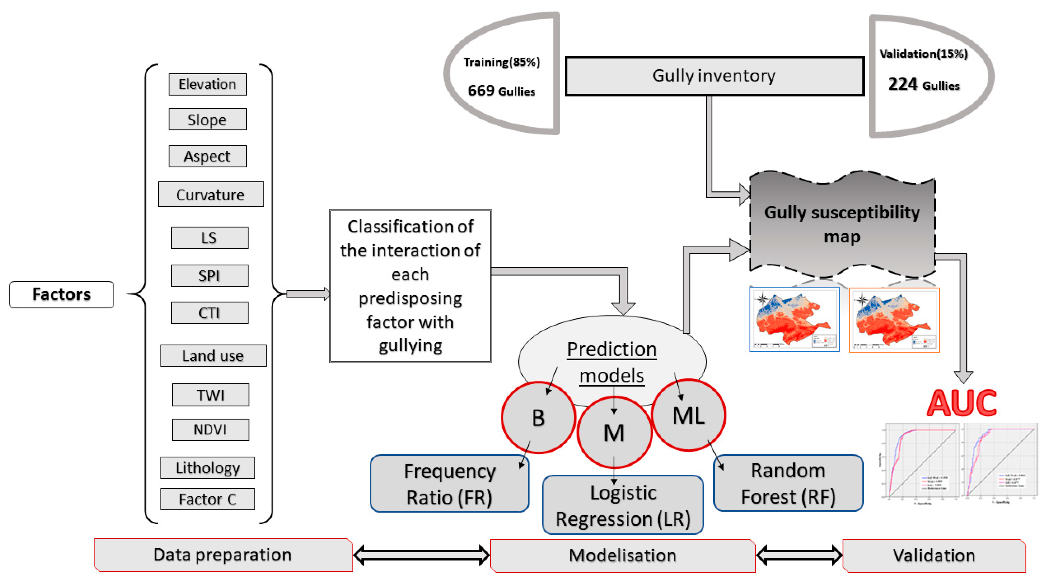
2. Materials and Methods
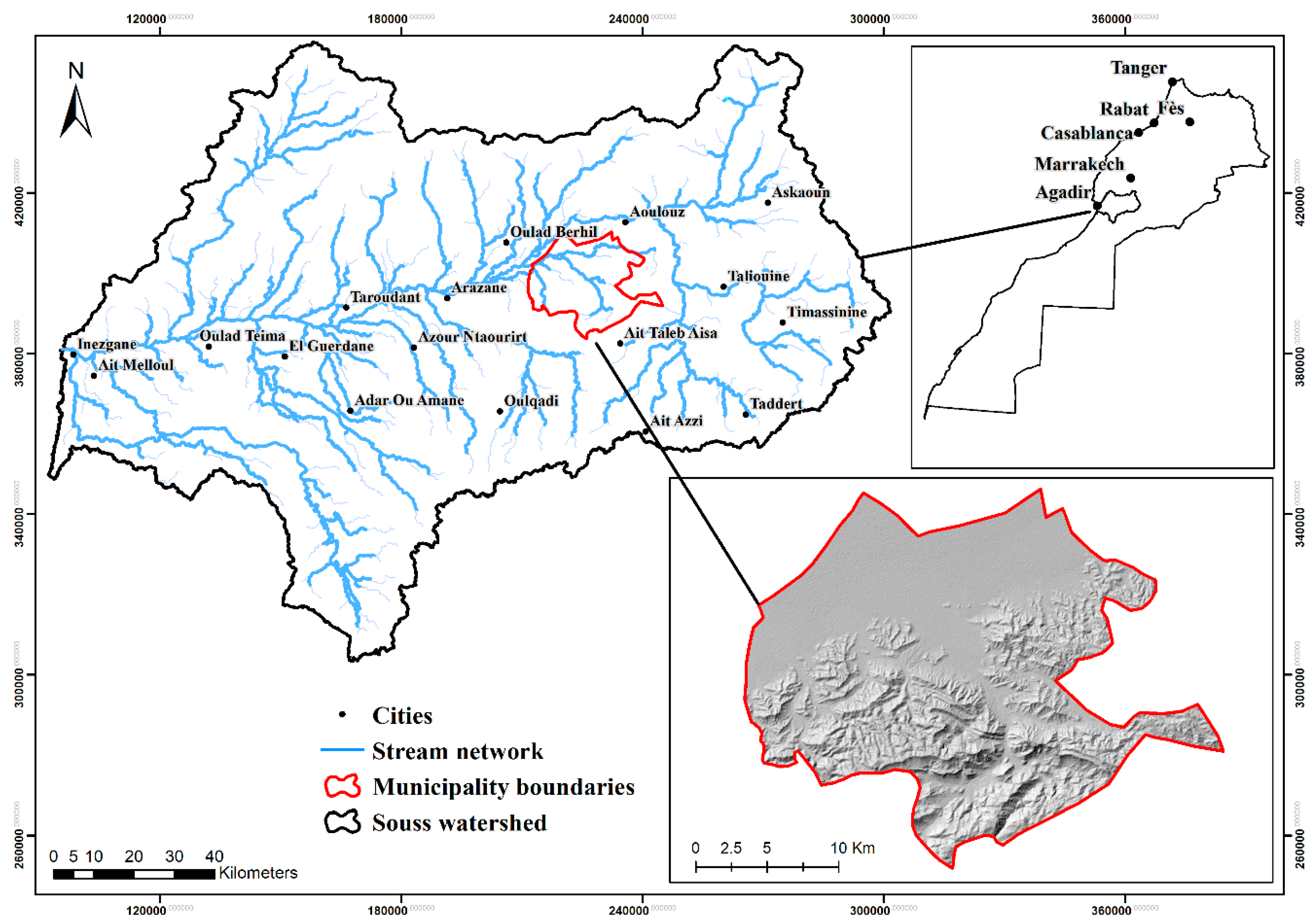
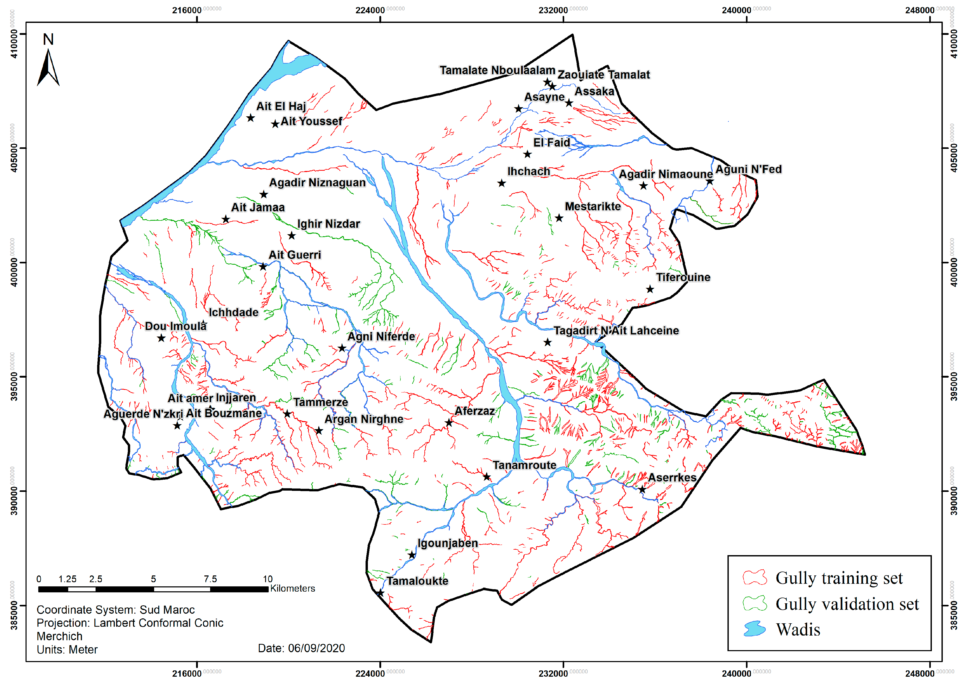
2.1. Study Area
2.2. Methods
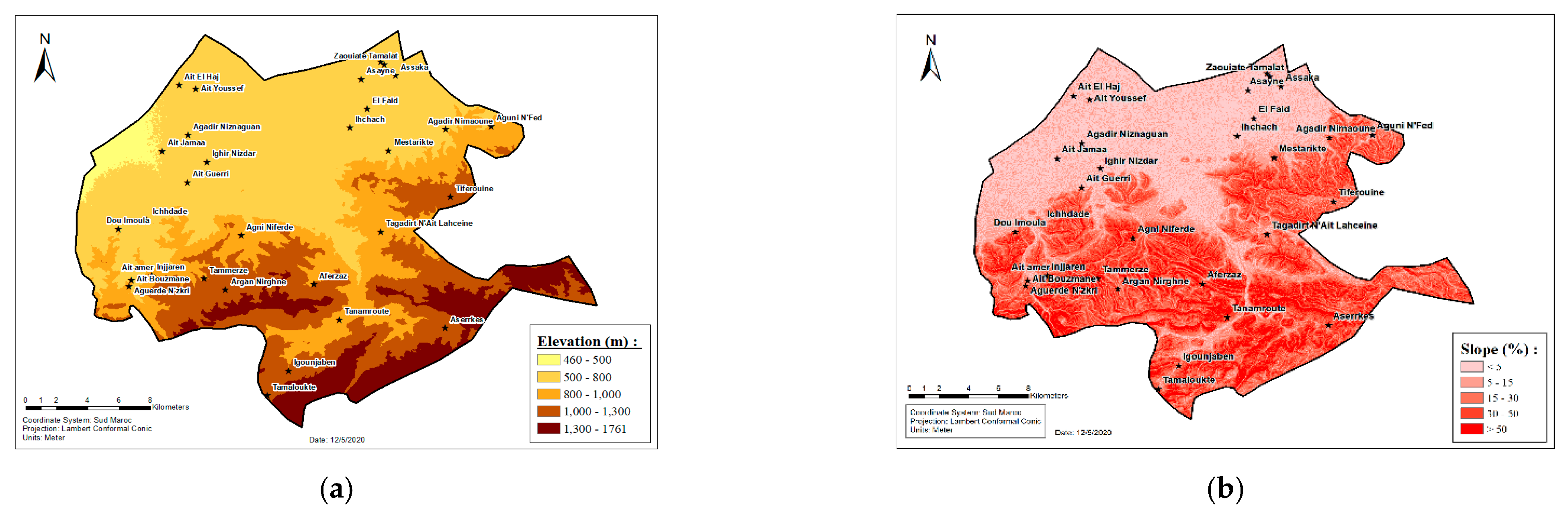
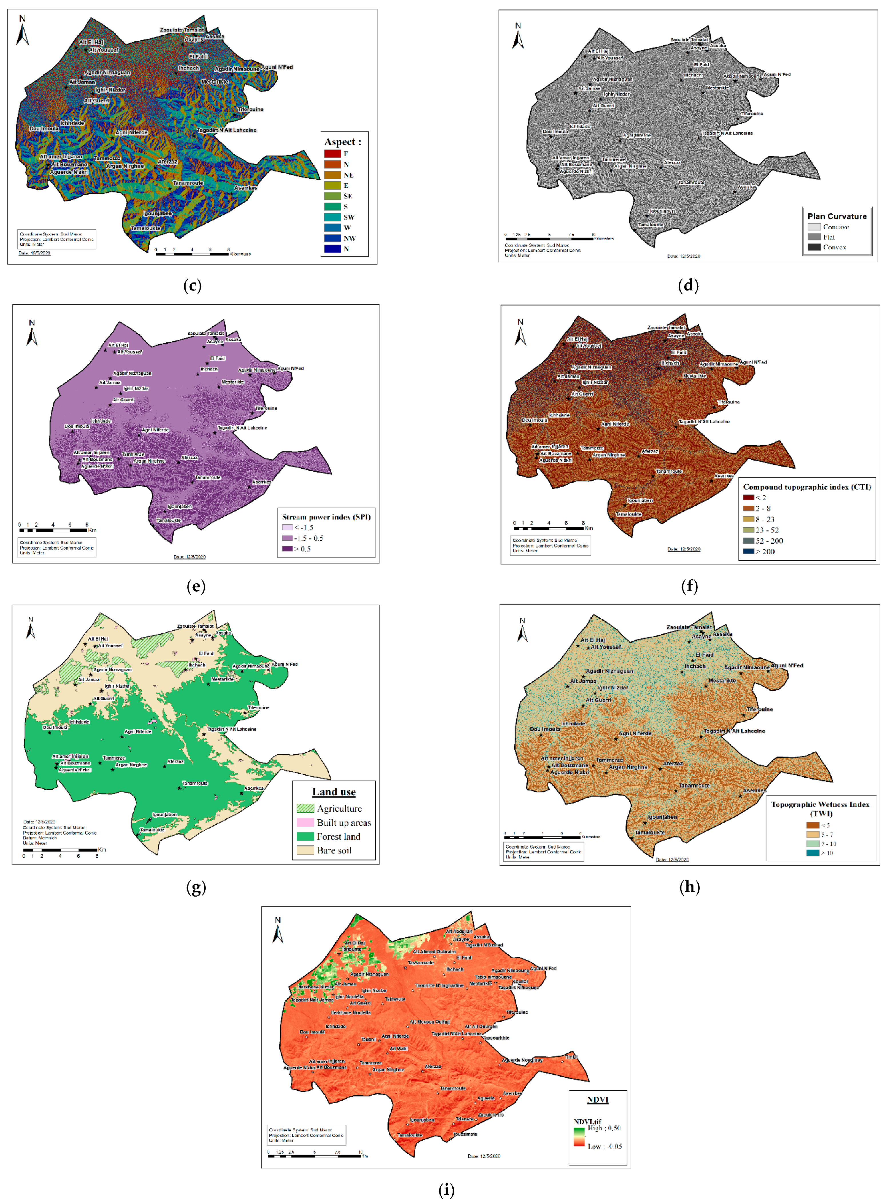
2.2.1. Used Data
2.2.2. Gully Susceptibility Models
Background of the Modeling Approaches Used
Frequency Ratio (FR)
Logistic Regression (LR)
Random Forest (RF)
Data Set Preparation
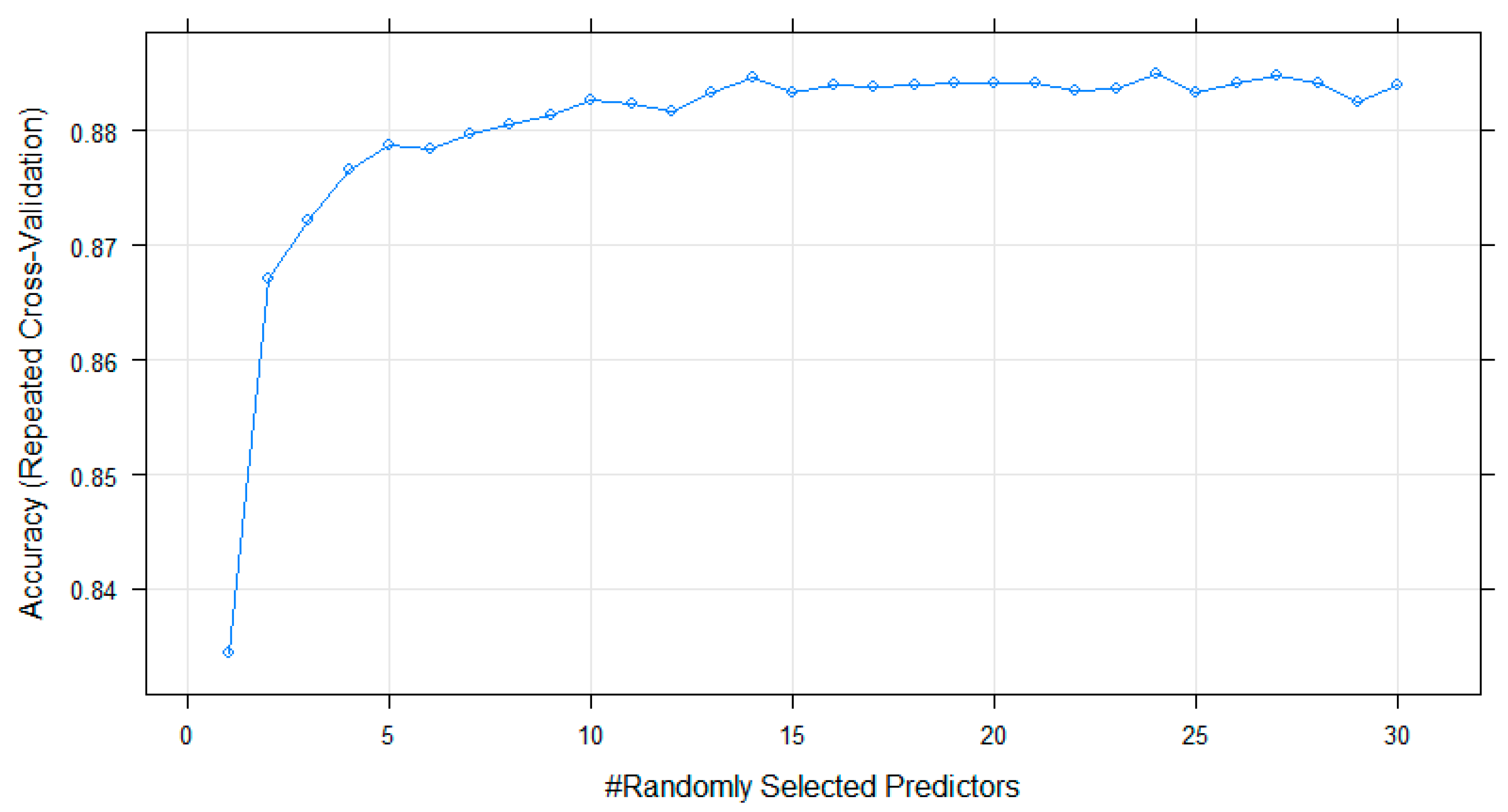
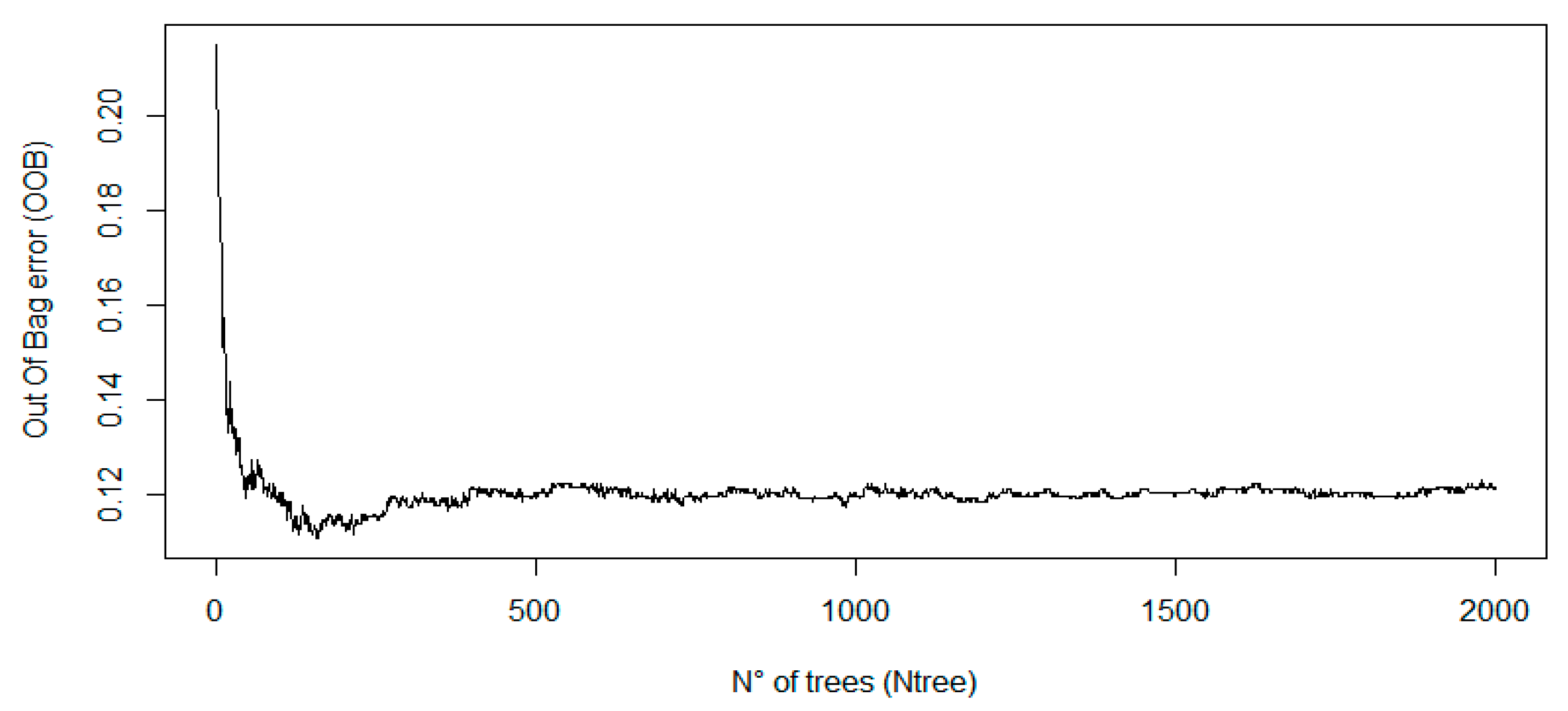
2.2.3. Optimizing and Tuning the Models
2.2.4. Susceptibility Model Validation
3. Results
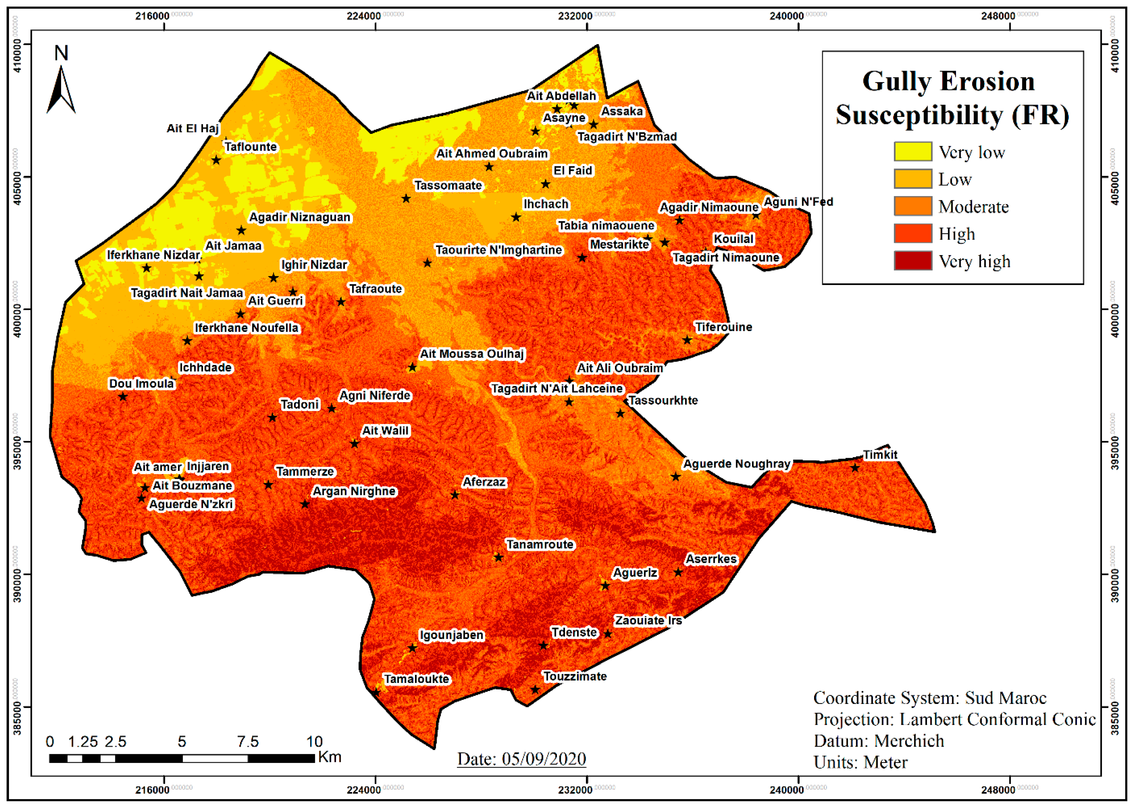
3.1. Gully Erosion Susceptibility Modeling
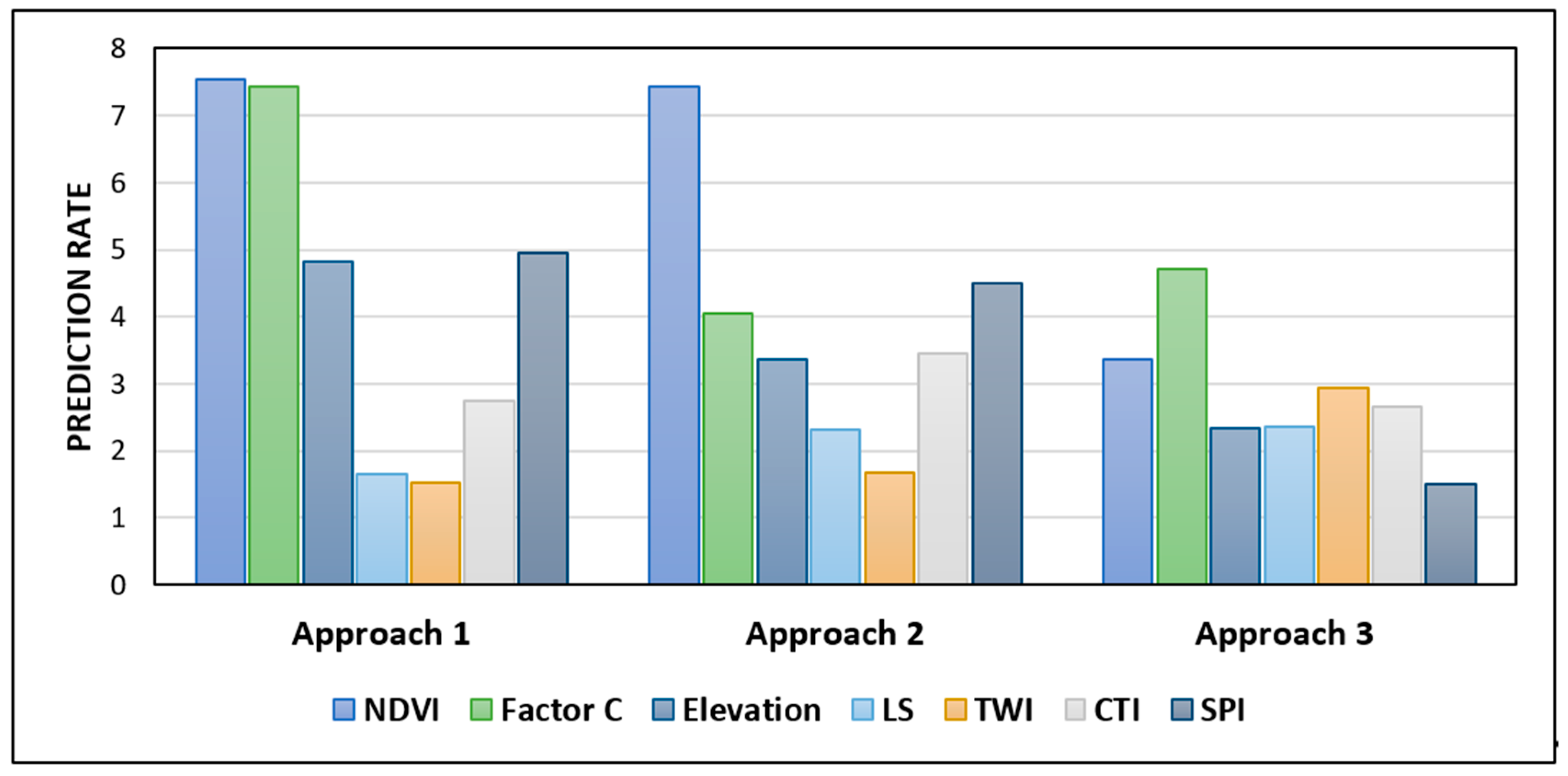
3.1.1. Effect of the Classification of Controlling Factors on the Predictive Performance of the Frequency Ratio Model
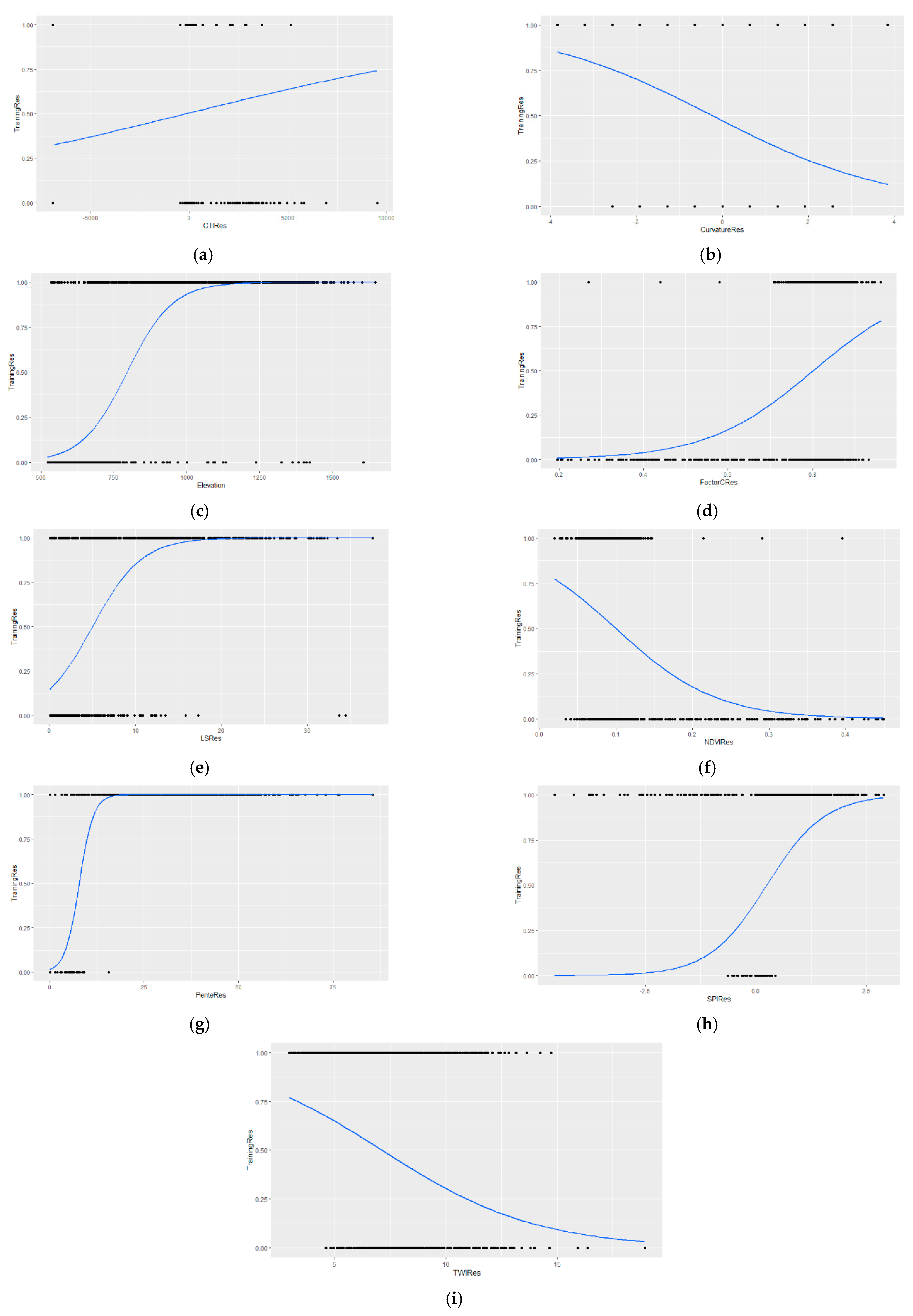
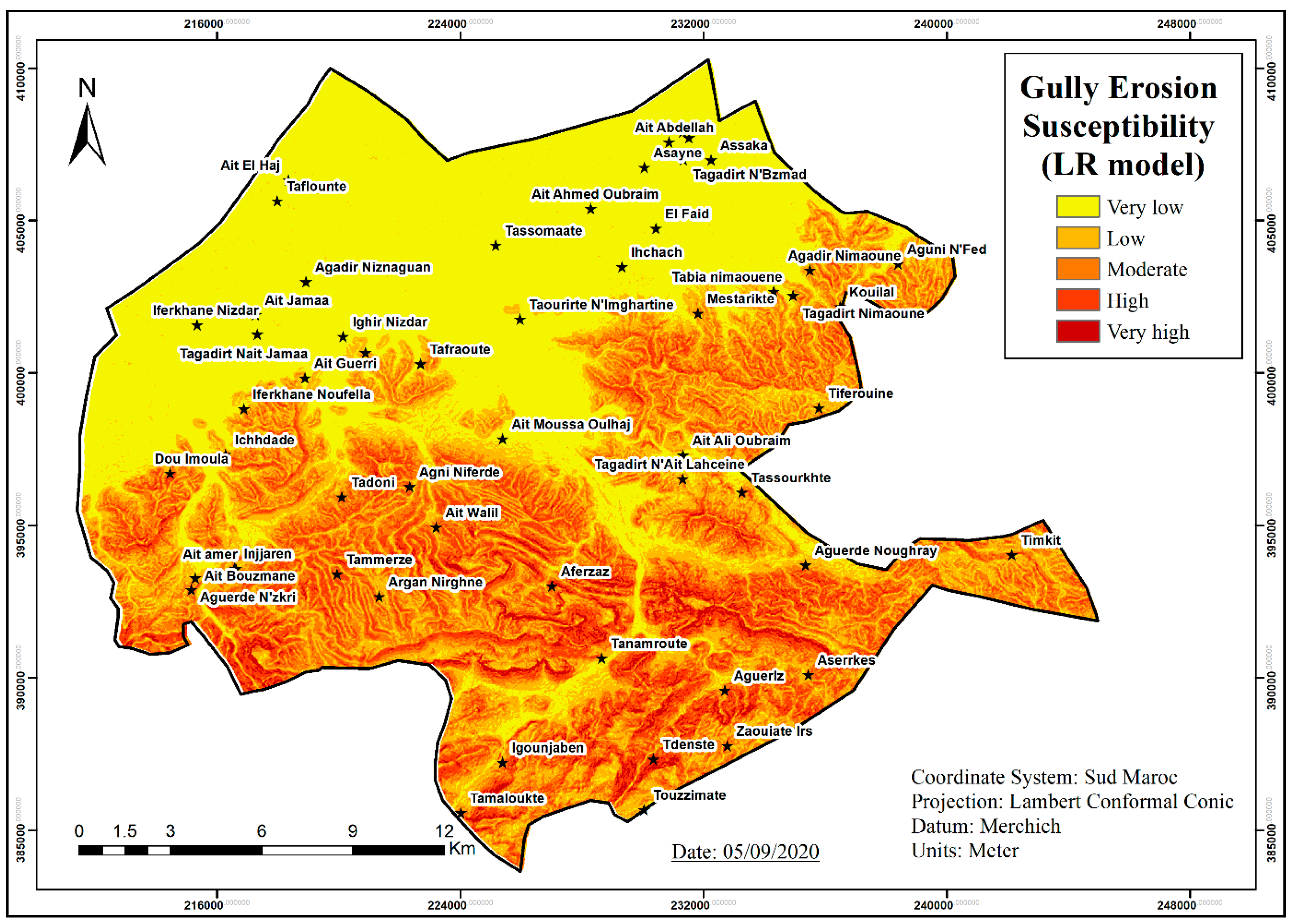
3.1.2. Gully Susceptibility Analysis Using the LR Model
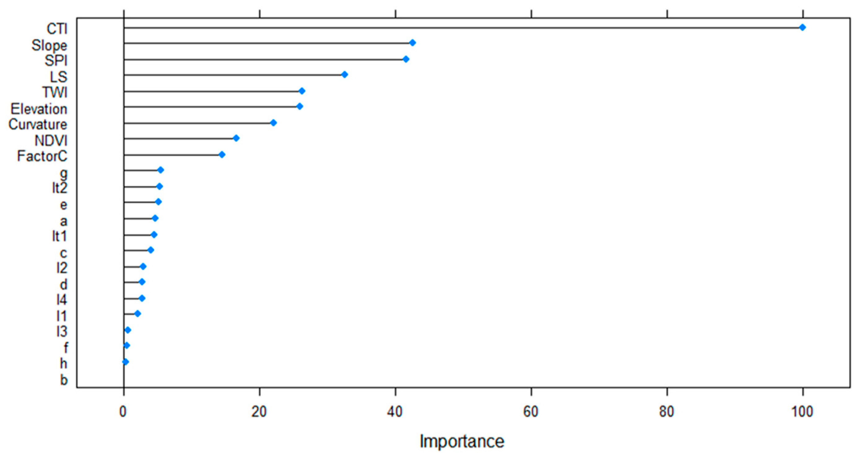
3.1.3. Gully susceptibility analysis using the RF model
3.2. Validating and Comparing the Models
3.2.1. FR Model Validation
3.2.2. LR Model Validation
3.2.3. RF Model Validation
3.3. Comparison between Models (FR, LR, and RF)
4. Discussion
5. Conclusions
Author Contributions
Funding
Institutional Review Board Statement
Informed Consent Statement
Data Availability Statement
Acknowledgments
Conflicts of Interest
References
- Alibou, J. Impacts des changements climatiques sur les ressources en eau et les zones humides du Maroc. In Proceedings of the Table Ronde Régionale Méditerranée, Athens, Greece, 10–11 December 2002; pp. 1–39. [Google Scholar]
- Fouad, E.; Rachid, D.M.; Aziz, F. Gestion Economique Intégrée des Ressources en eau à L’échelle du Bassin de Sous-Massa. 2013. Available online: http://webagris.inra.org.ma/doc/awamia/12705.pdf (accessed on 20 December 2020).
- Poloczanska, E.; Mintenbeck, K.; Portner, H.O.; Roberts, D.; Levin, L.A. The IPCC Special Report on the Ocean and Cryosphere in a Changing Climate; AGU: Washington, DC, USA, 2018. [Google Scholar]
- Atmospheric Warming and the Amplification of Precipitation Extremes|Science. Available online: https://science.sciencemag.org/content/321/5895/1481.abstract (accessed on 11 October 2020).
- Driouech, F. Distribution des précipitations hivernales sur le Maroc dans le cadre d’un changement climatique: Descente d’échelle et incertitudes. Ph.D. Thesis, Institut National Polytechnique de Toulouse, Toulouse, France, 2010. [Google Scholar]
- Bank, W.; Group, W.B. Global Financial Development Report 2014: Financial Inclusion; World Bank Publications: Washington, DC, USA, 2013; ISBN 978-0-8213-9985-9. [Google Scholar]
- Magliulo, P. Assessing the susceptibility to water-induced soil erosion using a geomorphological, bivariate statistics-based approach. Environ. Earth Sci. 2012, 67, 1801–1820. [Google Scholar] [CrossRef]
- Barakat, A.; Ouargaf, Z.; Khellouk, R.; Jazouli, A.E.; Touhami, F. Land Use/Land Cover Change and Environmental Impact Assessment in Béni-Mellal District (Morocco) Using Remote Sensing and GIS. Earth Syst. Environ. 2019, 3, 113–125. [Google Scholar] [CrossRef]
- UN Environment. Emissions Gap Report. 2018. Available online: http://www.unenvironment.org/resources/emissions-gap-report-2018 (accessed on 11 October 2020).
- Simonneaux, V.; Cheggour, A.; Deschamps, C.; Mouillot, F.; Cerdan, O.; Le Bissonnais, Y. Land use and climate change effects on soil erosion in a semi-arid mountainous watershed (High Atlas, Morocco). J. Arid Environ. 2015, 122, 64–75. [Google Scholar] [CrossRef] [Green Version]
- Soil Degradation by erosion-Lal-2001-Land Degradation & Development. Available online: https://0-onlinelibrary-wiley-com.brum.beds.ac.uk/doi/abs/10.1002/ldr.472 (accessed on 11 October 2020).
- Nampak, H.; Pradhan, B.; Rizeei, H.M.; Park, H.-J. Assessment of land cover and land use change impact on soil loss in a tropical catchment by using multitemporal SPOT-5 satellite images and Revised Universal Soil Loss Equation model. Land Degrad. Dev. 2018, 29, 3440–3455. [Google Scholar] [CrossRef]
- Termeh, S.V.R.; Niaraki, A.S.; Choi, S.-M. Gully erosion susceptibility mapping using artificial intelligence and statistical models. Geomat. Nat. Hazards Risk 2020, 11, 821–845. [Google Scholar] [CrossRef]
- Kheir, R.B.; Wilson, J.; Deng, Y. Use of terrain variables for mapping gully erosion susceptibility in Lebanon. Earth Surf. Process. Landf. 2007, 32, 1770–1782. [Google Scholar] [CrossRef]
- Rahmati, O.; Haghizadeh, A.; Pourghasemi, H.R.; Noormohamadi, F. Gully erosion susceptibility mapping: The role of GIS-based bivariate statistical models and their comparison. Nat. Hazards 2016, 82, 1231–1258. [Google Scholar] [CrossRef]
- McCloskey, G.L.; Wasson, R.J.; Boggs, G.S.; Douglas, M. Timing and causes of gully erosion in the riparian zone of the semi-arid tropical Victoria River, Australia: Management implications. Geomorphology 2016, 266, 96–104. [Google Scholar] [CrossRef]
- Foster, G.R. Understanding Ephemeral Gully Erosion. Soil Conservation: Assessing the National Research Inventory, National Research Council, Board on Agriculture 2; National Academy Press: Washington, DC, USA, 1986. [Google Scholar]
- Laflen, J.M.; Shaw, R.R. Ephemeral Gully Erosion Model (EGEM) Version 1.1 User Manual; USDA Soil Conservation Service: Washington, DC, USA, 1988.
- Rahmati, O.; Pourghasemi, H.R.; Melesse, A.M. Application of GIS-based data driven random forest and maximum entropy models for groundwater potential mapping: A case study at Mehran Region, Iran. Catena 2016, 137, 360–372. [Google Scholar] [CrossRef]
- Descroix, L.; Nouvelot, J.-F.; Vauclin, M. Evaluation of an antecedent precipitation index to model runoff yield in the western Sierra Madre (North-west Mexico). J. Hydrol. 2002, 263, 114–130. [Google Scholar] [CrossRef]
- Castillo, V.M.; Plaza, A.G.; Mena, M.M. The role of antecedent soil water content in the runoff response of semiarid catchments: A simulation approach. J. Hydrol. 2003, 284, 114–130. [Google Scholar] [CrossRef]
- Capra, A.; Ferro, V.; Porto, P.; Scicolone, B. Quantifying interrill and ephemeral gully erosion in a small Sicilian basin interrill and ephemeral gully erosion in a small Sicilian basin. Z. Für Geomorphol. Suppl. Issues 2012, 56, 9–25. [Google Scholar] [CrossRef] [Green Version]
- Cui, P.; Lin, Y.; Chen, C. Destruction of vegetation due to geo-hazards and its environmental impacts in the Wenchuan earthquake areas. Ecol. Eng. 2012, 44, 61–69. [Google Scholar] [CrossRef]
- Maaoui, M.A.E.; Felfoul, M.S.; Boussema, M.R.; Snane, M.H. Sediment yield from irregularly shaped gullies located on the Fortuna lithologic formation in semi-arid area of Tunisia. Catena 2012, 93, 97–104. [Google Scholar] [CrossRef]
- Oltmanns, S.O.D.; Marzolff, I.; Tiede, D.; Blaschke, T. Detection of Gully-Affected Areas by Applying Object-Based Image Analysis (OBIA) in the Region of Taroudannt, Morocco. Remote Sens. 2014, 6, 8287–8309. [Google Scholar] [CrossRef] [Green Version]
- Dube, F.; Nhapi, I.; Murwira, A.; Gumindoga, W.; Goldin, J.; Mashauri, D.A. Potential of weight of evidence modelling for gully erosion hazard assessment in Mbire District—Zimbabwe. Phys. Chem. Earth Parts ABC 2014, 67–69, 145–152. [Google Scholar] [CrossRef]
- Conoscenti, C.; Angileri, S.; Cappadonia, C.; Rotigliano, E.; Agnesi, V.; Märker, M. Gully erosion susceptibility assessment by means of GIS-based logistic regression: A case of Sicily (Italy). Geomorphology 2014, 204, 399–411. [Google Scholar] [CrossRef] [Green Version]
- Arabameri, A.; Chen, W.; Loche, M.; Zhao, X.; Li, Y.; Lombardo, L.; Cerda, A.; Pradhan, B.; Bui, D.T. Comparison of machine learning models for gully erosion susceptibility mapping. Geosci. Front. 2020, 11, 1609–1620. [Google Scholar] [CrossRef]
- Gayen, A.; Pourghasemi, H.R.; Saha, S.; Keesstra, S.; Bai, S. Gully erosion susceptibility assessment and management of hazard-prone areas in India using different machine learning algorithms. Sci. Total Environ. 2019, 668, 124–138. [Google Scholar] [CrossRef]
- Lei, X.; Chen, W.; Avand, M.; Janizadeh, S.; Kariminejad, N.; Shahabi, H.; Costache, R.; Shahabi, H.; Shirzadi, A.; Mosavi, A. GIS-Based Machine Learning Algorithms for Gully Erosion Susceptibility Mapping in a Semi-Arid Region of Iran. Remote Sens. 2020, 12, 2478. [Google Scholar] [CrossRef]
- Gafurov, A.M.; Yermolayev, O.P. Automatic Gully Detection: Neural Networks and Computer Vision. Remote Sens. 2020, 12, 1743. [Google Scholar] [CrossRef]
- Saadat, H.; Adamowski, J.; Tayefi, V.; Namdar, M.; Sharifi, F.; Ale-Ebrahim, S. A new approach for regional scale interrill and rill erosion intensity mapping using brightness index assessments from medium resolution satellite images. Catena 2014, 113, 306–313. [Google Scholar] [CrossRef]
- Gutierrez, A.G.; Schnabel, S.; Felicísimo, Á.M. Modelling the occurrence of gullies in rangelands of southwest Spain. Earth Surf. Process. Landf. J. Br. Geomorphol. Res. Group 2009, 34, 1894–1902. [Google Scholar] [CrossRef]
- Lucà, F.; Conforti, M.; Robustelli, G. Comparison of GIS-based gullying susceptibility mapping using bivariate and multivariate statistics: Northern Calabria, South Italy. Geomorphology 2011, 134, 297–308. [Google Scholar] [CrossRef]
- Zabihi, M.; Mirchooli, F.; Motevalli, A.; Darvishan, A.K.; Pourghasemi, H.R.; Zakeri, M.A.; Sadighi, F. Spatial modelling of gully erosion in Mazandaran Province, northern Iran. Catena 2018, 161, 1–13. [Google Scholar] [CrossRef]
- Shahabi, H.; Hashim, M.; Ahmad, B.B. Remote sensing and GIS-based landslide susceptibility mapping using frequency ratio, logistic regression, and fuzzy logic methods at the central Zab basin, Iran. Environ. Earth Sci. 2015, 73, 8647–8668. [Google Scholar] [CrossRef]
- Sahana, M.; Sajjad, H. Evaluating effectiveness of frequency ratio, fuzzy logic and logistic regression models in assessing landslide susceptibility: A case from Rudraprayag district, India. J. Mt. Sci. 2017, 14, 2150–2167. [Google Scholar] [CrossRef]
- Meliho, M.; Khattabi, A.; Mhammdi, N. A GIS-based approach for gully erosion susceptibility modelling using bivariate statistics methods in the Ourika watershed, Morocco. Environ. Earth Sci. 2018, 77, 655. [Google Scholar] [CrossRef]
- Gutiérrez, Á.G.; Schnabel, S.; Contador, J.F.L. Using and comparing two nonparametric methods (CART and MARS) to model the potential distribution of gullies. Ecol. Model. 2009, 220, 3630–3637. [Google Scholar] [CrossRef]
- Rahmati, O.; Tahmasebipour, N.; Haghizadeh, A.; Pourghasemi, H.R.; Feizizadeh, B. Evaluation of different machine learning models for predicting and mapping the susceptibility of gully erosion. Geomorphology 2017, 298, 118–137. [Google Scholar] [CrossRef]
- Pourghasemi, H.R.; Yousefi, S.; Kornejady, A.; Cerdà, A. Performance assessment of individual and ensemble data-mining techniques for gully erosion modeling. Sci. Total Environ. 2017, 609, 764–775. [Google Scholar] [CrossRef] [PubMed] [Green Version]
- Arabameri, A.; Yamani, M.; Pradhan, B.; Melesse, A.; Shirani, K.; Bui, D.T. Novel ensembles of COPRAS multi-criteria decision-making with logistic regression, boosted regression tree, and random forest for spatial prediction of gully erosion susceptibility. Sci. Total Environ. 2019, 688, 903–916. [Google Scholar] [CrossRef] [PubMed]
- Adelabu, S.; Dube, T. Employing ground and satellite-based QuickBird data and random forest to discriminate five tree species in a Southern African Woodland. Geocarto Int. 2015, 30, 457–471. [Google Scholar] [CrossRef]
- Hong, H.; Tsangaratos, P.; Ilia, I.; Chen, W.; Xu, C. Comparing the performance of a logistic regression and a random forest model in landslide susceptibility assessments. The Case of Wuyaun Area, China. In Proceedings of the Workshop on World landslide Forum, Ljubljana, Slovenia, 29 May–2 June 2017; pp. 1043–1050. [Google Scholar]
- Pardeshi, S.D.; Autade, S.E.; Pardeshi, S.S. Landslide hazard assessment: Recent trends and techniques. SpringerPlus 2013, 2, 523. [Google Scholar] [CrossRef] [PubMed] [Green Version]
- Abadi, A.M.A.; Ali, A.K.A. Susceptibility mapping of gully erosion using GIS-based statistical bivariate models: A case study from Ali Al-Gharbi District, Maysan Governorate, southern Iraq. Environ. Earth Sci. 2018, 77, 249. [Google Scholar] [CrossRef]
- Süzen, M.L.; Doyuran, V. A comparison of the GIS based landslide susceptibility assessment methods: Multivariate versus bivariate. Environ. Geol. 2004, 45, 665–679. [Google Scholar] [CrossRef]
- Conforti, M.; Robustelli, G.; Muto, F.; Critelli, S. Application and validation of bivariate GIS-based landslide susceptibility assessment for the Vitravo river catchment (Calabria, south Italy). Nat. Hazards 2012, 61, 127–141. [Google Scholar] [CrossRef]
- Azareh, A.; Rahmati, O.; Sardooi, E.R.; Sankey, J.B.; Lee, S.; Shahabi, H.; Ahmad, B.B. Modelling gully-erosion susceptibility in a semi-arid region, Iran: Investigation of applicability of certainty factor and maximum entropy models. Sci. Total Environ. 2019, 655, 684–696. [Google Scholar] [CrossRef]
- Bui, D.T.; Shirzadi, A.; Shahabi, H.; Chapi, K.; Omidavr, E.; Pham, B.T.; Talebpour Asl, D.; Khaledian, H.; Pradhan, B.; Panahi, M.; et al. A Novel Ensemble Artificial Intelligence Approach for Gully Erosion Mapping in a Semi-Arid Watershed (Iran). Sensors 2019, 19, 2444. [Google Scholar] [CrossRef] [Green Version]
- Pham, B.T.; Jaafari, A.; Prakash, I.; Bui, D.T. A novel hybrid intelligent model of support vector machines and the MultiBoost ensemble for landslide susceptibility modeling. Bull. Eng. Geol. Environ. 2019, 78, 2865–2886. [Google Scholar] [CrossRef]
- Kuhnert, P.M.; Henderson, A.-K.; Bartley, R.; Herr, A. Incorporating uncertainty in gully erosion calculations using the random forests modelling approach. Environmetrics 2010, 21, 493–509. [Google Scholar] [CrossRef]
- Eustace, A.H.; Pringle, M.J.; Denham, R.J. A risk map for gully locations in central Queensland, Australia. Eur. J. Soil Sci. 2011, 62, 431–441. [Google Scholar] [CrossRef]
- Nhu, V.-H.; Shirzadi, A.; Shahabi, H.; Chen, W.; Clague, J.J.; Geertsema, M.; Jaafari, A.; Avand, M.; Miraki, S.; Talebpour Asl, D.; et al. Shallow Landslide Susceptibility Mapping by Random Forest Base Classifier and Its Ensembles in a Semi-Arid Region of Iran. Forests 2020, 11, 421. [Google Scholar] [CrossRef] [Green Version]
- Sahin, E.K.; Colkesen, I.; Kavzoglu, T. A comparative assessment of canonical correlation forest, random forest, rotation forest and logistic regression methods for landslide susceptibility mapping. Geocarto Int. 2020, 35, 341–363. [Google Scholar] [CrossRef]
- Vafakhah, M.; Loor, S.M.H.; Pourghasemi, H.; Katebikord, A. Comparing performance of random forest and adaptive neuro-fuzzy inference system data mining models for flood susceptibility mapping. Arab. J. Geosci. 2020, 13, 417. [Google Scholar] [CrossRef]
- Nguyen, P.T.; Ha, D.H.; Nguyen, H.D.; van Phong, T.; Trinh, P.T.; Ansari, N.A.; Le, H.V.; Pham, B.T.; Ho, L.S.; Prakash, I. Improvement of Credal Decision Trees Using Ensemble Frameworks for Groundwater Potential Modeling. Sustainability 2020, 12, 2622. [Google Scholar] [CrossRef] [Green Version]
- Shruthi, R.B.; Kerle, N.; Jetten, V.; Stein, A. Object-based gully system prediction from medium resolution imagery using Random Forests. Geomorphology 2014, 216, 283–294. [Google Scholar] [CrossRef]
- Tairi, A.; Elmouden, A.; Aboulouafa, M. Soil Erosion Risk Mapping Using the Analytical Hierarchy Process (AHP) and Geographic Information System in the Tifnout-Askaoun Watershed, Southern Morocco. Eur. Sci. J. 2019, 15, 1857–7881. [Google Scholar] [CrossRef] [Green Version]
- Ambroggi, R. Etude Géologique du Versant Méridional du Haut Atlas Occidental et de la Plaine du Souss; Editions du Service géologique du Maroc: Rabat, Morocoo, 1963. [Google Scholar]
- Bocco, G. Gully erosion: Processes and models. Prog. Phys. Geogr. Earth Environ. 1991, 15, 392–406. [Google Scholar] [CrossRef]
- Poesen, J.; Vanwalleghem, T.; Deckers, J. Gullies and Closed Depressions in the Loess Belt: Scars of Human–Environment Interactions. In Landscapes and Landforms of Belgium and Luxembourg; Springer: Cham, Switzerland, 2018; pp. 253–267. [Google Scholar]
- Valentin, C.; Poesen, J.; Li, Y. Gully erosion: Impacts, factors and control. Catena 2005, 63, 132–153. [Google Scholar] [CrossRef]
- Conforti, M.; Aucelli, P.P.; Robustelli, G.; Scarciglia, F. Geomorphology and GIS analysis for mapping gully erosion susceptibility in the Turbolo stream catchment (Northern Calabria, Italy). Nat. Hazards 2011, 56, 881–898. [Google Scholar] [CrossRef]
- Jaafari, A.; Najafi, A.; Rezaeian, J.; Sattarian, A. Modeling erosion and sediment delivery from unpaved roads in the north mountainous forest of Iran. GEM Int. J. Geomath. 2015, 6, 343–356. [Google Scholar] [CrossRef]
- Gutiérrez, Á.G.; Conoscenti, C.; Angileri, S.E.; Rotigliano, E.; Schnabel, S. Using topographical attributes to evaluate gully erosion proneness (susceptibility) in two mediterranean basins: Advantages and limitations. Nat. Hazards 2015, 79, 291–314. [Google Scholar] [CrossRef]
- Zhou, P.; Luukkanen, O.; Tokola, T.; Nieminen, J. Effect of vegetation cover on soil erosion in a mountainous watershed. Catena 2008, 75, 319–325. [Google Scholar] [CrossRef]
- Moore, I.D.; Grayson, R.B.; Ladson, A.R. Digital terrain modelling: A review of hydrological, geomorphological, and biological applications. Hydrol. Process. 1991, 5, 3–30. [Google Scholar] [CrossRef]
- Parker, C.; Thorne, C.; Bingner, R.; Wells, R.; Wilcox, D. Automated Mapping of the Potential for Ephemeral Gully Formation in Agricultural Watersheds; National Sedimentation Laboratory: Oxford, MS, USA, 2007.
- Beven, K.J.; Kirkby, M.J. A physically based, variable contributing area model of basin hydrology/Un modèle à base physique de zone d’appel variable de l’hydrologie du bassin versant. Hydrol. Sci. J. 1979, 24, 43–69. [Google Scholar] [CrossRef] [Green Version]
- Bean, T.A.; Sumner, P.D.; Boojhawon, R.; Tatayah, V.; Khadun, A.K.; Hedding, D.W.; Rughooputh, S.; Nel, W. Bedrock-incised gully erosion phenomena on Round Island, Mauritius. Catena 2017, 151, 107–117. [Google Scholar] [CrossRef]
- Pourghasemi, H.R.; Rossi, M. Landslide susceptibility modeling in a landslide prone area in Mazandarn Province, north of Iran: A comparison between GLM, GAM, MARS, and M-AHP methods. Theor. Appl. Climatol. 2017, 130, 609–633. [Google Scholar] [CrossRef]
- Wells, R.R.; Bennett, S.J.; Alonso, C.V. Effect of soil texture, tailwater height, and pore-water pressure on the morphodynamics of migrating headcuts in upland concentrated flows. Earth Surf. Process. Landf. 2009, 34, 1867–1877. [Google Scholar] [CrossRef]
- Agnesi, V.; Angileri, S.; Cappadonia, C.; Conoscenti, C.; Rotigliano, E. Multi parametric gis analysis to assess gully erosion susceptibility: A test in southern sicily, italy. Landf. Anal. 2011, 17, 15–20. [Google Scholar]
- Bryan, R.B.; Jones, J.A.A. The significance of soil piping processes: Inventory and prospect. Geomorphol. Amst. 1997, 20, 209–218. [Google Scholar] [CrossRef]
- Geissen, V.; Kampichler, C.; López-de Llergo-Juárez, J.J.; Acántara, A.G. Superficial and subterranean soil erosion in Tabasco, tropical Mexico: Development of a decision tree modeling approach. Geoderma 2007, 139, 277–287. [Google Scholar] [CrossRef]
- Deng, Q.; Qin, F.; Zhang, B.; Wang, H.; Luo, M.; Shu, C.; Liu, H.; Liu, G. Characterizing the morphology of gully cross-sections based on PCA: A case of Yuanmou Dry-Hot Valley. Geomorphology 2015, 228, 703–713. [Google Scholar] [CrossRef]
- Okereke, C.N.; Onu, N.N.; Akaolisa, C.Z.; Ikoro, D.O.; Ibeneme, S.I.; Ubechu, B.; Chinemelu, E.S.; Amadikwa, L.O. Mapping gully erosion using remote sensing technique: A case study of Okigwe area, southeastern Nigeria. Int. J. Eng. Res. Appl. 2012, 2, 1955–1967. [Google Scholar]
- Yalcin, A.; Reis, S.; Aydinoglu, A.C.; Yomralioglu, T. A GIS-based comparative study of frequency ratio, analytical hierarchy process, bivariate statistics and logistics regression methods for landslide susceptibility mapping in Trabzon, NE Turkey. Catena 2011, 85, 274–287. [Google Scholar] [CrossRef]
- Lee, S.; Talib, J.A. Probabilistic landslide susceptibility and factor effect analysis. Environ. Geol. 2005, 47, 982–990. [Google Scholar] [CrossRef]
- Pradhan, B.; Lee, S. Landslide susceptibility assessment and factor effect analysis: Backpropagation artificial neural networks and their comparison with frequency ratio and bivariate logistic regression modelling. Environ. Model. Softw. 2010, 25, 747–759. [Google Scholar] [CrossRef]
- Althuwaynee, O.F.; Pradhan, B.; Park, H.-J.; Lee, J.H. A novel ensemble bivariate statistical evidential belief function with knowledge-based analytical hierarchy process and multivariate statistical logistic regression for landslide susceptibility mapping. Catena 2014, 114, 21–36. [Google Scholar] [CrossRef]
- Breiman, L. Random forests. Mach. Learn. 2001, 45, 5–32. [Google Scholar] [CrossRef] [Green Version]
- Arabameri, A.; Rezaei, K.; Pourghasemi, H.R.; Lee, S.; Yamani, M. GIS-based gully erosion susceptibility mapping: A comparison among three data-driven models and AHP knowledge-based technique. Environ. Earth Sci. 2018, 77, 628. [Google Scholar] [CrossRef]
- Arabameri, A.; Pradhan, B.; Rezaei, K. Gully erosion zonation mapping using integrated geographically weighted regression with certainty factor and random forest models in GIS. J. Environ. Manag. 2019, 232, 928–942. [Google Scholar] [CrossRef] [PubMed]
- Roy, J.; Saha, D.S. GIS-based Gully Erosion Susceptibility Evaluation Using Frequency Ratio, Cosine Amplitude and Logistic Regression Ensembled with fuzzy logic in Hinglo River Basin, India. Remote Sens. Appl. Soc. Environ. 2019, 15, 100247. [Google Scholar] [CrossRef]
- Ozdemir, A.; Altural, T. A comparative study of frequency ratio, weights of evidence and logistic regression methods for landslide susceptibility mapping: Sultan Mountains, SW Turkey. J. Asian Earth Sci. 2013, 64, 180–197. [Google Scholar] [CrossRef]
- Arabameri, A.; Pradhan, B.; Rezaei, K.; Yamani, M.; Pourghasemi, H.R.; Lombardo, L. Spatial modelling of gully erosion using evidential belief function, logistic regression, and a new ensemble of evidential belief function–logistic regression algorithm. Land Degrad. Dev. 2018, 29, 4035–4049. [Google Scholar] [CrossRef]
- Momm, H.G.; Bingner, R.L.; Wells, R.R.; Wilcox, D. AGNPS GIS-based tool for watershed-scale identification and mapping of cropland potential ephemeral gullies. Appl. Eng. Agric. 2012, 28, 17–29. [Google Scholar] [CrossRef] [Green Version]
- Termeh, S.V.R.; Kornejady, A.; Pourghasemi, H.R.; Keesstra, S. Flood susceptibility mapping using novel ensembles of adaptive neuro fuzzy inference system and metaheuristic algorithms. Sci. Total Environ. 2018, 615, 438–451. [Google Scholar] [CrossRef] [PubMed]
- Yesilnacar, E.K. The Application of Computational Intelligence to Landslide Susceptibility Napping in Turkey; University of Melbourne, Department: Melbourne, VIC, Australia, 2005; p. 200. [Google Scholar]
- Moukrim, S.; Lahssini, S.; Alaoui, H.M.; Rifai, N.; Arahou, M.; Rhazi, L. Modélisation de la distribution spatiale des espèces endémiques pour leur conservation: Cas de l’Argania spinosa (L.) Skeels. Rev. Décologie 2018, 73, 153–166. [Google Scholar]
- Stehman, S.V. Selecting and interpreting measures of thematic classification accuracy. Remote Sens. Environ. 1997, 62, 77–89. [Google Scholar] [CrossRef]
- Pourghasemi, H.R.; Sadhasivam, N.; Kariminejad, N.; Collins, A.L. Gully erosion spatial modelling: Role of machine learning algorithms in selection of the best controlling factors and modelling process. Geosci. Front. 2020, 11, 2207–2219. [Google Scholar] [CrossRef]
- Lombardo, L.; Fubelli, G.; Amato, G.; Bonasera, M. Presence-only approach to assess landslide triggering-thickness susceptibility: A test for the Mili catchment (north-eastern Sicily, Italy). Nat. Hazards 2016, 84, 565–588. [Google Scholar] [CrossRef]
- Rahmati, O.; Kornejady, A.; Samadi, M.; Deo, R.C.; Conoscenti, C.; Lombardo, L.; Dayal, K.; Taghizadeh-Mehrjardi, R.; Pourghasemi, H.R.; Kumar, S.; et al. PMT: New analytical framework for automated evaluation of geo-environmental modelling approaches. Sci. Total Environ. 2019, 664, 296–311. [Google Scholar] [CrossRef]
- Rasyid, A.R.; Bhandary, N.P.; Yatabe, R. Performance of frequency ratio and logistic regression model in creating GIS based landslides susceptibility map at Lompobattang Mountain, Indonesia. Geoenviron. Disasters 2016, 3, 19. [Google Scholar] [CrossRef] [Green Version]
- Pradhan, B. Remote sensing and GIS-based landslide hazard analysis and cross-validation using multivariate logistic regression model on three test areas in Malaysia. Adv. Space Res. 2010, 45, 1244–1256. [Google Scholar] [CrossRef]
- Lee, S.; Pradhan, B. Landslide hazard mapping at Selangor, Malaysia using frequency ratio and logistic regression models. Landslides 2007, 4, 33–41. [Google Scholar] [CrossRef]
- Süzen, M.L.; Kaya, B.Ş. Evaluation of environmental parameters in logistic regression models for landslide susceptibility mapping. Int. J. Digit. Earth 2012, 5, 338–355. [Google Scholar] [CrossRef]
- Meten, M.; Bhandary, N.P.; Yatabe, R. GIS-based frequency ratio and logistic regression modelling for landslide susceptibility mapping of Debre Sina area in central Ethiopia. J. Mt. Sci. 2015, 12, 1355–1372. [Google Scholar] [CrossRef]
- Chen, W.; Zhang, S.; Li, R.; Shahabi, H. Performance evaluation of the GIS-based data mining techniques of best-first decision tree, random forest, and naïve Bayes tree for landslide susceptibility modeling. Sci. Total Environ. 2018, 644, 1006–1018. [Google Scholar] [CrossRef]
- Rizeei, H.M.; Pradhan, B.; Saharkhiz, M.A. An integrated fluvial and flash pluvial model using 2D high-resolution sub-grid and particle swarm optimization-based random forest approaches in GIS. Complex Intell. Syst. 2019, 5, 283–302. [Google Scholar] [CrossRef] [Green Version]
- Arabameri, A.; Pradhan, B.; Pourghasemi, H.R.; Rezaei, K.; Kerle, N. Spatial Modelling of Gully Erosion Using GIS and R Programing: A Comparison among Three Data Mining Algorithms. Appl. Sci. 2018, 8, 1369. [Google Scholar] [CrossRef] [Green Version]
- Zhang, X.; Fan, J.; Liu, Q.; Xiong, D. The contribution of gully erosion to total sediment production in a small watershed in Southwest China. Phys. Geogr. 2018, 39, 246–263. [Google Scholar]


| Factor | Form and Resolution | Source |
|---|---|---|
| Elevation, slope, aspect, plan curvature, LS, SPI, CTI, and TWI | 12.5 × 12.5 m | DEM (ALOS PALSAR) https://search.asf.alaska.edu/ |
| Land use, factor C, NDVI, | 10 × 10 m | Sentinel-2, imagery of 07-04-2019 https://earthexplorer.usgs.gov/ |
| Lithology | 12.5 × 12.5 m | Geological map of Marrakech at a 1:500,000 scale, produced in 1957 |
| N Class | Classified | Bare Soils | Built-Up Areas | Agriculture | Forrested Areas | Total | Corrected Sample |
|---|---|---|---|---|---|---|---|
| 1 | Bare soils | 81 | 7 | 8 | 8 | 104 | 81 |
| 2 | Built-up areas | 2 | 14 | 7 | 5 | 28 | 14 |
| 3 | Agriculture | 1 | 0 | 18 | 11 | 30 | 18 |
| 4 | Forested areas | 2 | 4 | 3 | 79 | 88 | 79 |
| Total | 86 | 25 | 36 | 103 | 250 | 192 | |
| Overall accuracy (A) | 0.768 | ||||||
| Kappa | 0.661 | ||||||
| Type of Rock | Lithofacies | Description |
|---|---|---|
| Limestone | Very high | Unaltered compact rock, conglomerates or strongly cemented soils (massif, limestone, strongly stony soils, igneous or eruptive rocks) |
| Marls, sandstone, silts | Low | Moderately compacted sedimentary rocks and soils. Soil or soft rock, weakly resistant or strongly/deeply altered (marls, gypsum, clay, silt, etc.) |
| Land Use | Lithology | Aspect | ||||||||||||
|---|---|---|---|---|---|---|---|---|---|---|---|---|---|---|
| L1 | L2 | L3 | L4 | Lt1 | Lt2 | a | b | c | d | e | f | g | h | |
| Class | Bare soil | Built-up areas | Agricultural land | Forest | Marls, sandstone, silts | Limestone | North | North-East | East | South-East | South | South-West | West | North-West |
| Factor | Approach 1 | Approach 2 | Approach 3 |
|---|---|---|---|
| NDVI | <−0.03 | <0.14 | <0.05 |
| −0.03–0.13 | 0.14–0.27 | 0.05–0.1 | |
| >0.13 | >0.27 | 0.1–0.2 | |
| 0.2–0.3 | |||
| >0.3 | |||
| C factor | <0.5 | <0.6 | <0.2 |
| 0.5–0.7 | 0.6–0.8 | 0.2–0.4 | |
| >0.7 | >0.8 | 0.4–0.6 | |
| 0.6–0.8 | |||
| >0.8 | |||
| Elevation (m) | <600 | <827 | <600 |
| 600–1200 | 827–1164 | 600–800 | |
| > 1200 | >1164 | 800–1000 | |
| 1000–1200 | |||
| 1200–1400 | |||
| >1400 | |||
| LS | <2 | <3.4 | <2 |
| 2–5 | 3.4–8.7 | 2–5 | |
| 5–10 | 8.7–13.9 | 5–12 | |
| 10–15 | 13.9–19.6 | 12–20 | |
| >15 | >19.6 | >20 | |
| TWI | <5 | <4.7 | <2 |
| 5–7 | 4.7–7.4 | 2–5 | |
| 7–10 | 7.4–10.3 | 5–7 | |
| >10 | >10.3 | 7–10 | |
| >10 | |||
| CTI | <2 | <−387.8 | <−250 |
| 2–8 | −387.8–−196.9 | −250–−50 | |
| 8–23 | −196.9–−11.6 | −50–0 | |
| 23–52 | −11.6–15.3 | 0–10 | |
| 52–198 | 15.3–56.9 | 10–25 | |
| >198 | >56.9 | 25–50 | |
| 50–100 | |||
| >100 | |||
| SPI | <1.5 | <−1.3 | <0 |
| 1.5–2 | −1.3–0.3 | 0–0.5 | |
| >2 | >0.3 | 0.5–1 | |
| 1–2 | |||
| > 2 | |||
| Slope (%) | <5 | ||
| 5–15 | |||
| 15–30 | |||
| 30–50 | |||
| >50 [39,65,85] | |||
| Aspect | Flat | ||
| North | |||
| North-East | |||
| East | |||
| South-East | |||
| South | |||
| South-West | |||
| West | |||
| North-West | |||
| Land use | Bare soils | ||
| Built-up areas | |||
| Agriculture | |||
| Forested areas | |||
| Curvature Plan | Concave | ||
| Flat | |||
| Convex | |||
| Lithology | Marls, sandstone and silts | ||
| Limestone | |||
| Approach 1 | Approach 2 | Approach 3 | |||||||
|---|---|---|---|---|---|---|---|---|---|
| Factors | Classes | FR | PR | Classes | FR | PR | Classes | FR | PR |
| NDVI | <−0.03 | 0.00 | 7.53 | <0.14 | 0.86 | 7.44 | <0.05 | 0.30 | 3.36 |
| −0.03–0.13 | 0.84 | 0.14–0.27 | 0.04 | 0.05–0.1 | 0.28 | ||||
| >0.13 | 0.16 | >0.27 | 0.10 | 0.1–0.2 | 0.38 | ||||
| 0.2–0.3 | 0.03 | ||||||||
| >0.3 | 0.01 | ||||||||
| Factor C | <0.5 | 0.08 | 7.42 | <0.6 | 0.04 | 4.06 | <0.2 | 0.00 | 4.71 |
| 0.5–0.7 | 0.05 | 0.6–0.8 | 0.49 | 0.2–0.4 | 0.02 | ||||
| >0.7 | 0.87 | >0.8 | 0.47 | 0.4–0.6 | 0.02 | ||||
| 0.6–0.8 | 0.55 | ||||||||
| >0.8 | 0.41 | ||||||||
| Elevation (m) | <600 | 0.06 | 4.81 | <827 | 0.09 | 3.37 | <600 | 0.02 | 2.35 |
| 600–1200 | 0.35 | 827–1164 | 0.45 | 600–800 | 0.05 | ||||
| >1200 | 0.59 | >1164 | 0.46 | 800–1000 | 0.21 | ||||
| 1000–1200 | 0.26 | ||||||||
| 1200–1400 | 0.29 | ||||||||
| >1400 | 0.17 | ||||||||
| LS | <2 | 0.10 | 1.65 | <3.4 | 0.06 | 2.32 | <2 | 0.05 | 2.36 |
| 2–5 | 0.13 | 3.4–8.7 | 0.32 | 2–5 | 0.26 | ||||
| 5–10 | 0.22 | 8.7–13.9 | 0.29 | 5–12 | 0.31 | ||||
| 10–15 | 0.27 | 13.9–19.6 | 0.21 | 12–20 | 0.25 | ||||
| >15 | 0.28 | >19.6 | 0.12 | > 20 | 0.13 | ||||
| TWI | <5 | 0.15 | 1.52 | <4.7 | 0.15 | 1.67 | <2 | 0.07 | 2.93 |
| 5–7 | 0.20 | 4.7–7.4 | 0.20 | 2–5 | 0.37 | ||||
| 7–10 | 0.32 | 7.4–10.3 | 0.32 | 5–7 | 0.28 | ||||
| >10 | 0.33 | >10.3 | 0.33 | 7–10 | 0.20 | ||||
| >10 | 0.08 | ||||||||
| CTI | <2 | 0.07 | 2.75 | <−387.8 | 0.05 | 3.45 | <−250 | 0.02 | 2.66 |
| 2–8 | 0.21 | −387.8–−196.9 | 0.00 | −250–−50 | 0.05 | ||||
| 8–23 | 0.35 | −196.9–−11.6 | 0.14 | −50–0 | 0.10 | ||||
| 23–52 | 0.20 | −11.6–15.3 | 0.30 | 0–10 | 0.15 | ||||
| 52–198 | 0.13 | 15.3–56.9 | 0.38 | 10–25 | 0.32 | ||||
| 198< | 0.04 | 56.9< | 0.13 | 25–50 | 0.17 | ||||
| 50–100 | 0.13 | ||||||||
| >100 | 0.06 | ||||||||
| SPI | <1.5 | 0.12 | 4.95 | <−1.3 | 0.21 | 4.49 | <0 | 0.05 | 1.51 |
| 1.5–2 | 0.20 | −1.3–0.3 | 0.15 | 0–0.5 | 0.07 | ||||
| >2 | 0.68 | >0.3 | 0.64 | 0.5–1 | 0.22 | ||||
| 1–2 | 0.29 | ||||||||
| >2 | 0.37 | ||||||||
| Slope (%) | <5 | 0.04 | 2.91 | ||||||
| 5–15 | 0.15 | ||||||||
| 15–30 | 0.36 | ||||||||
| 30–50 | 0.28 | ||||||||
| >50 | 0.17 | ||||||||
| Aspect | Flat | 0.08 | 1.00 | ||||||
| North | 0.14 | ||||||||
| North- East | 0.10 | ||||||||
| East | 0.07 | ||||||||
| South-East | 0.12 | ||||||||
| South | 0.18 | ||||||||
| South-West | 0.11 | ||||||||
| West | 0.10 | ||||||||
| North-West | 0.10 | ||||||||
| Land use | Bare soils | 0.36 | 5.57 | ||||||
| Built-up areas | 0.00 | ||||||||
| Agriculture | 0.02 | ||||||||
| Forested areas | 0.62 | ||||||||
| Curvature plan | Concave | 0.54 | 3.07 | ||||||
| Flat | 0.26 | ||||||||
| Convex | 0.20 | ||||||||
| Lithology | Marls, sandstone and silts | 0.11 | 6.96 | ||||||
| Limestone | 0.89 | ||||||||
| Factors | Estimated Weight | Standard Error |
|---|---|---|
| Aspect | −1.321 × 10⁻³ | 1.188 × 10⁻³ |
| CTI | −4.676 × 10⁻⁵ | 8.423 × 10⁻⁵ |
| Curvatureplan | −1.623 × 10⁻¹ | 1.983 × 10⁻¹ |
| Elevation | 2.698 × 10⁻³ | 8.713 × 10⁻⁴ |
| Factor C | −4.510 × 101 | 4.777 × 10+1 |
| Land use | 2.029 × 10⁻¹ | 1.194 × 10⁻¹ |
| Lithology | 4.140 × 10⁻¹ | 4.298 × 10⁻¹ |
| LS factor | 6.188 × 10⁻² | 3.608 × 10⁻² |
| NDVI | −8.484 × 101 | 8.967 × 10+1 |
| Slope | 4.813 × 10⁻¹ | 5.572 × 10⁻² |
| SPI | −8.804 × 10⁻¹ | 8.474 × 10⁻¹ |
| TWI | 2.698 × 10⁻¹ | 9.320 × 10⁻² |
| p-value = 0.0093 | ||
| (FR) | Class Error | (LR) | Class Error | (RF) | Class Error | |||||
|---|---|---|---|---|---|---|---|---|---|---|
| No Gully | Gully | No Gully | Gully | No Gully | Gully | |||||
| Prediction | No Gullying | 41.50% | 11.30% | 21.40% | 49.14% | 0.81% | 1.60% | 68.69 | 0.63% | 0.90% |
| Gullying | 8.50% | 38.70% | 18% | 4.30% | 46.83% | 6.40% | 0.95% | 29.71 | 3.10% | |
| Accuracy | 80.20% | 95.98% | 98.4 | |||||||
Publisher’s Note: MDPI stays neutral with regard to jurisdictional claims in published maps and institutional affiliations. |
© 2021 by the authors. Licensee MDPI, Basel, Switzerland. This article is an open access article distributed under the terms and conditions of the Creative Commons Attribution (CC BY) license (http://creativecommons.org/licenses/by/4.0/).
Share and Cite
Azedou, A.; Lahssini, S.; Khattabi, A.; Meliho, M.; Rifai, N. A Methodological Comparison of Three Models for Gully Erosion Susceptibility Mapping in the Rural Municipality of El Faid (Morocco). Sustainability 2021, 13, 682. https://0-doi-org.brum.beds.ac.uk/10.3390/su13020682
Azedou A, Lahssini S, Khattabi A, Meliho M, Rifai N. A Methodological Comparison of Three Models for Gully Erosion Susceptibility Mapping in the Rural Municipality of El Faid (Morocco). Sustainability. 2021; 13(2):682. https://0-doi-org.brum.beds.ac.uk/10.3390/su13020682
Chicago/Turabian StyleAzedou, Ali, Said Lahssini, Abdellatif Khattabi, Modeste Meliho, and Nabil Rifai. 2021. "A Methodological Comparison of Three Models for Gully Erosion Susceptibility Mapping in the Rural Municipality of El Faid (Morocco)" Sustainability 13, no. 2: 682. https://0-doi-org.brum.beds.ac.uk/10.3390/su13020682